Hierarchical Decision Making In Electricity Grid Management

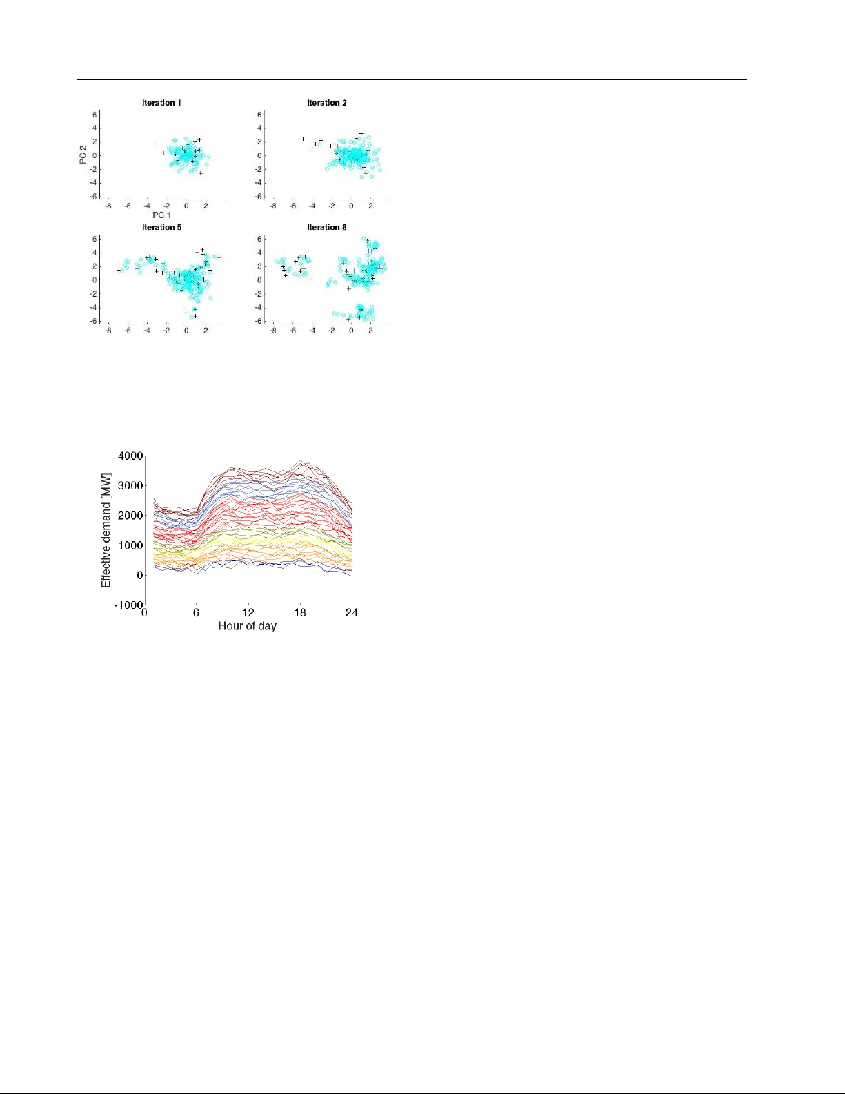
Hierar chical Decision Making In Electricity Grid Management Gal Dalal G A L D @ T X . T E C H N I O N . AC . I L T echnion, Israel Elad Gilboa E G I L B OA @ T X . T E C H N I O N . A C . I L T echnion, Israel Shie Mannor S H I E @ E E . T E C H N I O N . AC . I L T echnion, Israel Abstract The power grid is a comple x and vital sys- tem that necessitates careful reliability manage- ment. Managing the grid is a dif ficult prob- lem with multiple time scales of decision making and stochastic behavior due to rene wable energy generations, v ariable demand and unplanned out- ages. Solving this problem in the face of uncer- tainty requires a ne w methodology with tractable algorithms. In this work, we introduce a ne w model for hierarchical decision making in com- plex systems. W e apply reinforcement learning (RL) methods to learn a pr oxy , i.e., a le vel of ab- straction, for real-time po wer grid reliability . W e devise an algorithm that alternates between slo w time-scale policy improv ement, and fast time- scale v alue function approximation. W e compare our results to pre v ailing heuristics, and sho w the strength of our method. 1. Introduction The power grid is a complex and vital system that requires high lev el of reliability . Reliability is of utmost importance, as the consequences of outages can be catastrophic. System operators (SOs) achie ve reliability by means of sophisti- cated control operations and planning, which often require solving sequential stochastic decision problems. Sequen- tial decision making under uncertainty in energy systems is studied in different communities such as control theory , dynamic programming, stochastic programming and ro- bust optimization ( Powell & Meisel , 2015 ; Bertsimas et al. , 2013 ; Bienstock , 2011 ; K outsopoulos & T assiulas , 2012 ; Pr oceedings of the 33 rd International Conference on Machine Learning , New Y ork, NY , USA, 2016. JMLR: W&CP volume 48. Copyright 2016 by the author(s). Bienstock et al. , 2014 ). Reliability assessment and control are highly complicated tasks in complex real-world systems such as the po wer grid. Complications in the power grid arise because of strict physical restrictions, such as generation must meet consumption continuously and transmission lines can not exceed their limited thermal capacity . Further complica- tions stem from the structure of decision making in dif- ferent time-horizons. For example, long-term system ex- pansion and development such as building a new wind farm or a high-voltage line tak e years, mid-term asset man- agement decisions such as performing maintenance are decided upon months in advance, short-term generation schedules are planned daily , and real-time operational con- trol decisions are made on the scale of minutes. In these interdependent hierarchical decision making processes de- cisions are taken by multiple stakeholders. Furthermore, ov er the last decade, wind and solar energy sources become increasingly preeminent with further significant expansion being envisaged ( T albot , 2009 ). These generators intro- duce high uncertainty to the system, making the control task significantly more difficult. The complex dependence between multiple time-horizon with growing uncertainty , the curse of dimensionality when dealing with large sys- tems, and the non-linear dependence of reliability measures to the multiple time-horizon decisions, make this problem extremely hard to tackle. T o stress the dimensionality comple xity , consider the IEEE R TS-96 power network used in our experiments ( W ong et al. , 1999 ). This network is an example for a power grid of a medium sized European country or a state in the USA. Its state-space is O (10 300 ) , and its action space is O (10 100 ) ; see Sec. 5 . Assessment of each control choice carries a computational burden as it requires solving a set of non-linear trigonometric equations named alternating cur - rent power flo w (ACPF); see Sec. 2.1 . Hierarchical Decision Making In Electricity Grid Management Now adays, the common practice in industry is solving large mixed integer programs (MIP), often with a linear re- laxation, in an attempt to reach a v alid solution ( Grainger & Stev enson , 1994 ; Allan et al. , 2013 ). Although this model is extensi ve, its computational burden makes it hard ev en for deterministic predictions (taking an order of a day in real-world systems), and inappropriate in the stochastic case. This limits SOs to sample snapshots of future grid states or analyze a fe w sequential trajectories. The narrow view of possible outcomes is likely to miss important ben- efits and increase the costs of decisions, thereby offering little in terms of dealing with uncertainty . T o handle uncertainty , work has been done in stochastic optimization and control theory . These often use restrictive simplifications such as independence between the decision processes in the dif ferent time-scales or consider myopic decisions only ( Abiri-Jahromi et al. , 2009 ; W u et al. , 2010 ; Abiri-Jahromi et al. , 2013 ). Another approach is to use approximate dynamic program- ming ( Powell , 2007 ; Si , 2004 ). Howe ver , the natural hierar- chical structure of the problem, where se veral stak eholders operating in different time-scales and e xposed to different information are making decisions with mutual influence, does not naturally fit the standard Markov Decision Pro- cess (MDP) structure. Furthermore, the problem is heavily constrained, since physical electrical restrictions must be met at all times. Making this problem tractable requires a le vel of abstrac- tion in the form of fast proxy methods to approximate the impact of real-time decisions on longer-term reliability and costs. T o our knowledge, fe w attempts have been made to construct such proxies using tools from machine learning. An example for such, is the work conducted in a recent European project, iT esla ( iT e ). This work focuses on an- alyzing snapshots of system states at different time points using data-mining methods. Then, classification and clus- tering algorithms are used for constructing security rules for predicting reliability lev el, giv en a failure and an elec- trical network state ( Anil , 2013 ). Such approaches can aid SOs in real-time control, but lack the dynamic perspective of state-action ev olution needed to ev aluate consequences of policies in a sequential decision making scenario. In this work we suggest a novel approach to mitigate the intractability of the hierarchical decision making problem of the day-ahead (D A) and real-time (R T) reliability of the power grid. The contrib utions of our work are: • W e introduce an interleav ed MDPs hierarchical struc- ture with separate state space, action space, and re- ward metric. • W e devise an algorithm that alternates between high- lev el policy improvement and lower-le vel value ap- proximation, i.e., the policy improv ement in the first MDP is based on the second MDP’ s value function. • W e show the efficac y of our method on a medium- sized power grid problem. • W e introduce a new real-world application to the RL community and provide a simulation en vironment. The rest of paper is organized as follows. In Sec. 2 we present background on power system engineering. In Sec. 3 , we formulate the two-layer MDPs. In Sec. 4 , we introduce our interleav ed approximate policy improv ement (IAPI) algorithm and present results on the IEEE R TS-96 network. W e conclude our work in Sec. 6 . 2. Background In this section we present a brief introduction to the field of power systems engineering. This is v ast a field with exten- siv e background and theory . For more information please refer to ( Grainger & Stev enson , 1994 ; Allan et al. , 2013 ). 2.1. Decision Processes and Po wer Flow in Po wer Grids T o better explain the multiple time-horizon decision pro- cesses we use a toy 6-bus power grid example ( W ood & W ollenberg , 1996 ), shown in Fig. 1 . The 6-bus system is composed of 6 electrical nodes referred to as “b uses”. Each bus can hav e loads and generators attached to it. Loads (shown in blue) are consumers (e.g., large neighborhoods or cities and factories), and generators (shown in red) are power producers such as nuclear plants, coal plants, wind turbines, and solar panels. Load values change continu- ously throughout the day and closely follow daily , weekly , and yearly profiles. Controllable generators are operated such that the ov erall power generation meets the overall load at all times (up to transmission losses). The edges con- necting the buses represent transmission lines which, due to thermal restrictions, can only transfer a limited amount of power before risking tripping. Giv en a snapshot of loads and generation values, and the power grid topology (buses and transmission lines), it is possible to solve the complete alternating current power flow (ACPF) equations. The ACPF is a set of non-con vex trigonometric equations that model the physical electrical characteristics of the power grid, i.e., voltage magnitude and angles of each node ( Cain et al. , 2012 ). The A CPF so- lution includes the amount of power passing through each transmission line (shown in green in Fig. 1 ). In general, reliability of a power system is measured based on the avoidance of full or partial blackouts (both planned and unplanned) and their negati ve ef fect on social welfare. A blackout is an ev ent where demand cannot be met. This Hierarchical Decision Making In Electricity Grid Management Figure 1. W ood & W ollenberg 6-bus system, with generation val- ues in red; load v alues in green; and transmission line flow values in blue, obtained from an A C po wer-flo w solution. can occur predominantly because of contingencies (i.e., as- set malfunctions) which lead to unsafe operation and may require the SOs to disconnect loads in order to a v oid catas- trophes. Contingencies can stem from multiple causes, such as a tree falling, lighting strike, poor maintenance or exceeding the thermal limits of a transmission line. T o maintain a high reliability level at all times, the current practice of SOs is to immunize the system against a pre- determined contingenc y list. A common choice for this list is all single asset contingencies, resulting in the so-called N − 1 reliability criterion. Howe ver , contingency probabilities are dif ficult to ob- tain and their impact is hard to assess. Furthermore, the high penetration of stochastic and often uncontrollable re- new able generators, makes the planing tasks significantly harder for se veral reasons. First, generation must equal de- mand at all times. Second, multiple decision making pro- cesses are taking place simultaneously on multiple time- scales. Third, each decision process inv olv es high dimen- sional decision v ariables, and complex non-linear ( Powell & Meisel , 2015 ), often intractable mathematical formula- tions. For example, in the 6-bus system in Fig. 1 , a system de- veloper might plan to expand the system by b uilding a new transmission line between buses 3 and 4. Expanding the grid is a long term process and a decision must be taken years in adv ance. Howe v er , this decision affects the future maintenance decisions, which will affect future daily plan- ning that in turn affects the future real-time control room operations. Ideally , the system dev eloper should consider all possible future realizations of the en vironment, grid, and the decision processes in all other time horizons. 2.2. Related work Sev eral works in the literature of po wer systems, oper- ational research and more recently machine learning of- fer approaches for solving sequential stochastic problems using dynamic programming. Of which, the majority of these works focus on energy storage ( Lai et al. , 2010 ; Xi et al. , 2014 ; Jiang et al. , 2014 ; Scott & Powell , 2012 ), unit commitment ( Padhy , 2004 ; Dalal & Mannor , 2015 ; Ernst et al. , 2007 ), and ener gy market bidding strategies ( Song & W ang , 2003 ; Urieli & Stone , 2014 ; Jiang & Po well , 2015 ). T o our kno wledge, no work has been done to use MDPs for assessing the reliability in power grids. For our proxy abstraction de vise a hierarchical model. Hi- erarchical models, offer sev eral benefits over flat models when appropriate. They can improve exploration, enable learning from fe wer trials, and allow faster learning for ne w problems by reusing subtasks learned on previous problems ( Dietterich , 1998 ). Standard approaches for hierarchical models include: planning with options (often referred to as skills) ( Sutton et al. , 1999 ), task hierarchy ( Barto & Ma- hadev an , 2003 ) and hierarchy of abstract machines ( Parr & Russell , 1998 ). These models include levels of deci- sion making that share the same state-space and a termina- tion condition to switch between controllers. This structure does not fit our problem well where two separate decision makers run on differ ent state-spaces and temporal resolu- tions. 3. Problem F ormulation Here we present a formulation for the two sequential deci- sion processes occurring in the day ahead (D A) and real- time (R T) in terms of a hierarchal two MDP model. DA decisions are taken in order to maximize the system’ s next day reliability . Howe v er , the next day reliability can only be assessed in R T , and is dependent on the system opera- tor decision taken in R T . This results in a complex depen- dence between D A and R T actions and system reliability . W e therefore formulate the problem using two layers of interleav ed MDPs: a R T -MDP , describing the state of the system, reliability , and decisions on an hourly basis, and a D A-MDP describing the D A action of choosing a daily subset of active generators based on the upcoming day pre- dictions. In our terminology , the former serves as a pr oxy for assessing decisions taken in the latter , see Fig. 2 . 3.1. Day-Ahead MDP The D A-MDP is a tuple ( S D A , A D A , P D A , R D A ) . T ime in- dex is t d , denoting days. Day-ahead state s D A t d ∈ S D A con- sists of a day ahead prediction of hourly demand on each bus, and wind generation of each wind generator . 1 There- fore, S D A = R T D · ( n b + n g ) , where T D is the number of intra- day time steps ( 24 in our case), and n b , n g are the num- ber of buses and wind generators. For the day ahead ac- 1 In this work we consider only wind generation as a renewable source for simplicity . Hierarchical Decision Making In Electricity Grid Management Figure 2. Day-ahead and Real-Time hierarchical MDPs. The real- time process serves as a proxy for assessing decisions taken in day-ahead process. tion a D A t d ∈ A D A we use a simplified model which consid- ers a binary v ector indicating which generators participate in the next day’ s generation process. The sets of genera- tors contained in A D A represent common settings an SO can choose from. This set can be constructed by experts or inferred from data. An action a D A t d is chosen accord- ing to a policy a D A t d = π D A ( s D A t d ) . The next day state is chosen according to P D A , and is purely exogenous, i.e., P ( s D A t d +1 | s D A t d , a D A t d ) = P ( s D A t d +1 | s D A t d ) . The rew ard function R D A is a complicated function of the reliability in R T . Since we cannot obtain the day ahead reward directly , we re v ert to use the R T re ward as a surrogate for comparing D A poli- cies. Notice that we cannot directly use the sum of R T rew ards between consecuti v e days as a replacement for the D A re ward since the model will no longer be Mark ovian. 3.2. Real-Time MDP The R T -MDP is a tuple ( S R T , A R T , P R T , R R T ) . It repre- sents the real time reliability control process. T ime in- dex is t , denoting intra-day time steps (e.g., hours). In R T power network operation, an operator may choose preven- tiv e actions at each time step, trying to immunize the sys- tem against potential malfunctions by attempting to a void unreliable states. W e model this decision making process using post-states ( Powell , 2007 ), where at the beginning of each time interv al, the agent observes the current state s R T t ∈ S R T , i.e., the realized demand and wind values for this interval and chooses an action a R T t ∈ A R T . Follow- ing the agent’ s action, the system is now in a post-decision state s R T ,a t , which is the new state, after performing action a R T t from state s R T t . Next, e xogenous random information W t is obtained, informing whether equipment malfunction (contingency) occurred during time interval t . Given s R T ,a t and W t , the real time rew ard r R T t ( s R T ,a t , W t ) which rep- resents the system’ s reliability , can be calculated, and a transition to s R T t +1 occurs, go verned by P ( s R T t +1 | s R T ,a t , W t ) . The history of this R T process can be written as h R T t = ( s R T 0 , a R T 0 , s R T ,a 0 , W 0 , r R T 0 , s R T 1 , . . . , s R T t ) . 3 . 2 . 1 . R E A L - T I M E S TA T E S P AC E W e define a R T state s R T t to be the tuple ( d , w , g , e ) , where: d is a v ector of stochastic nodal demand. w is a vector of stochastic nodal wind generation. g is a vector of controllable generation values. The D A action a D A t d determines which generators will hav e pos- itiv e v alues, and which will be set to 0 throughout the day . Each generator has minimal and maximal genera- tion limits while in operation. e is the topology of the grid. Includes information of current state of each edge (transmission line). e ∈ { 0 , 1 , . . . , E } , where 0 is operational and the rest is a countdown process till the line is fix ed. 3 . 2 . 2 . R E A L - T I M E A C T I O N S P AC E A R T action a R T t is a preventi v e action, that attempts to achiev e better reliability of the system by immunizing against potential contingencies. The action in volves redis- patch ∆ g , i.e., change the generation v alues of the working controllable generators (chosen in D A): s R T t a R T t − − → s R T ,a t = ( d , w , g + ∆ g , e ) . Any action is allowed as long as it is within the minimal and maximal generator limits. Notice that ∆ g i 6 = 0 for working generators only ( a D A t d ,i = 1 ). 3 . 2 . 3 . R E A L - T I M E T R A N S I T I O N K E R N E L The R T transition kernel can be factorized to exogenous transitions of demand, wind generation, and contingencies. It is conditioned on the last R T state and action (encoded in the R T post-state), and on the corresponding last DA deci- sion taken to determine participating generators: s R T t +1 = f ( s R T ,a t , W t , a D A t d ) . The dependence between R T and DA states is expressed using two sets of equations. The first is R T demand process, based on D A demand prediction: d R T t = d D A t + δ t (1) δ t +1 = δ t +  t , (2) where d R T t is the R T demand vector at time t , and d D A t is the D A prediction vector for time t of the day . The dynamics in Eqs. ( 1 )-( 2 ) also hold for the wind generation process. For this work we chose this autoregressi v e random bias process for simplicity , howe ver more complicated methods, such as in ( Box et al. , 2015 ; Papav asiliou & Oren , 2013 ; T aylor & Buizza , 2002 ), can be considered. The second equation coupling D A and R T determines the generators participat- ing in current day generation process: g t +1 ,i = ( g t,i + ∆ g t,i if i ∈ I ( a D A t d ,i ) 0 otherwise , (3) Hierarchical Decision Making In Electricity Grid Management where I ( a D A t d ,i ) is the index set of generators chosen by D A action a D A t d ,i . Lastly , random e xogenous information W t specifies whether a contingency happened in the system, causing transmission line i to fail, changing the network topology to e t +1 . The probability of line i to fail at each time-step is p i if at the last time-step e i was 0 , and 0 otherwise. 3 . 2 . 4 . R E A L - T I M E R E W A R D W e choose the R T re ward to be the reliability lev el of the power system at the current time. T o assess the lev el of reliability , we employ the common criterion used in the in- dustry , termed N − 1 , which assesses the system ability to withstand any contingenc y of a single asset. T o calculate the reliability of the system, it is e xamined us- ing a sequence of tests (contingency list), where each test is an attempt to take out a single line (contingenc y) and check if the system retains safe operation. Hence, the rew ard r R T t ( s R T ,a t , W t ) is a number in [0 , 1] , expressing the por- tion of tests passed out of the predetermined contingency list, which includes all single contingencies c ∈ N − 1 . The reliability is calculated for a giv en state of the grid, and is dependent of current topology ( e t ) and the changes to the topology due to possible ne w contingencies ( W t ) . In practice, preserving the system in safe operation means be- ing able to obtain a feasible solution to the power flow equations (see Sec. 2 ) of the network circuit. W e define I [ PF ( c,s R T ,a t ,W t )] to be 1 if a power flo w solution exists, and 0 otherwise. As a result, the R T re ward is: r R T t ( s R T ,a t , W t ) = 1 |N − 1 | X c ∈N − 1 I [ PF ( c,s R T ,a t ,W t )] . 4. Interleav ed A pproximate P olicy Impro vement In this section we present our algorithm, called Inter- leaved Approximate P olicy Impr ovement (IAPI), presented in Alg. 1 , for jointly learning the R T reliability v alue func- tion while searching for an optimal DA policy . W e use the term interleaved since the policy improvement in one MDP is based on the second MDP’ s value function. W e use sim- ulation based value learning to assess the R T reliability of the system and the cross entropy method ( De Boer et al. , 2005 ; Szita & L ¨ orincz , 2006 ) for improving the D A pol- icy . Our method scales to large systems since it uses sim- ple models with carefully engineered features and design to run on distrib uted computing. Since the algorithm is mas- siv ely parallelizable, the more cores av ailable, the faster the con v ergence will be. Our goal is to find an optimal DA policy π D A , under the assumption that the R T policy π R T is known. Henceforth, we will use π to symbolize π D A . As e xplained in Sec. 3 , reliability is not explicitly defined on the D A lev el and we instead use the R T v alue function v π as a surrogate for com- paring between different DA policies. Differently than the common notation, v π denotes the R T value function, under the fixed R T policy π R T , and a D A polic y π . Algorithm 1 IAPI Algorithm Input: initial distribution P (0) ψ for D A polic y parameters Output: optimal D A policy π ( ψ ∗ ) 1: initialize S RT test = ∅ 2: repeat 3: for i ≤ N do 4: draw ψ i ∼ P ( k ) ψ 5: sample N episodes trajectories using π i = π ( ψ i ) 6: approximate v π i using TD(0) 7: add TD(0) trajectories to S RT test 8: end for 9: set empirical mean ˆ v ( k ) i = P s ∈S RT test v π i ( s ) , ∀ i ∈ [ N ] 10: rank policies π i according to ˆ v i 11: use ψ i of the top percentile π i to update P ( k ) ψ 12: k = k + 1 13: until con ver gence Our method includes the following components: Day Ahead Policy A pproximation W e de- fine a parametric D A policy as π ( s D A ; ψ ) = arg max a DA ∈A DA ψ > Φ( s D A , a D A ) , where a D A is the day ahead action dictating which generators will be active during the day , Φ( s D A , a D A ) are features of DA state s D A and action a D A . A plausible choice for mapping D A state s D A to an ac- tion a D A is using multi-class classifiers. Howe ver , for large number of classes ( 20 in our e xperiments) these methods require a significant number of simulations for training ( Bishop , 2006 ). Furthermore, approaches for classification-based policy learning often require obtaining multiple rollouts for all the actions from a state during the training procedure ( Gabillon et al. , 2011 ), which in our case will result in a full value ev aluation per each action and might prov e o verly encumbering. T o mitigate these com- plexities, our polic y chooses the action that maximizes the inner product with ψ . Real Time V alue Function Appr oximation F or a fixed D A policy π we approximate the R T v alue function using the TD(0) algorithm ( Sutton & Barto , 1998 ); see Fig 3 . The R T v alue function is parametrized as v π ( s R T ; θ π ) = θ > π φ ( s R T ) , with the parameter vector θ π depends on π , and φ ( s R T ) being the features of R T state s R T . Hierarchical Decision Making In Electricity Grid Management Figure 3. Day-ahead policy comparison using TD-learning of real-time value function. Day Ahead Policy Comparison A comparison between different D A policies π i is done by calculating the empiri- cal mean of R T value function E v π i ≈ P s ∈S R T test v π i ( s ) , us- ing a set of representati ve R T initial states S R T test . This set is composed of the full history of all R T states visited during the current IAPI iteration, enabling expected value estima- tion using many probable states with only linear computa- tional complexity in |S R T test | . Day Ahead Policy Improvement using Cross Entropy D A policy improvement is achieved using the cross en- tropy method ( De Boer et al. , 2005 ; Szita & L ¨ orincz , 2006 ). In this method, initial policies are sampled from a distri- bution P (0) ψ . F ollo wing which, in each iteration k pol- icy parameters ψ are drawn from P ( k ) ψ , and their top per - centile, according to the R T value, is used to update P ( k +1) ψ ( De Boer et al. , 2005 ; Szita & L ¨ orincz , 2006 ). In our e x- periments we set P (0) ψ such that it includes ψ that equally separate ψ > Φ( s D A 0 , a D A i ) , making this inner product equal, for all the dif ferent actions a D A i . The distrib ution P ( k ) ψ is a Gaussian mixture with means set to ψ ( k − 1) that be- long to the top percentile. The conv ergence criterion we use in our experiments with the difference between the top-percentile values average of two consecutive iterations 1 N top P N top i =1  ˆ v ( k ) i − ˆ v ( k − 1) i  2 <  . By using the cross en- tropy method, we av oid using gradient-based optimization which may be difficult to compute in our case due to the discrete, non-linear nature of A CPF solutions and their de- pendence of generation ( Cain et al. , 2012 ), which dictate the lev el of reliability . The criterion for comparing policies is a parametric R T value function, v π ( s R T ; θ π ) , as oppose to using rollouts for policy ev aluation ( Gabillon et al. , 2011 ). The reason for this choice is three-fold. First, since a rollout only explores a small part of the space, assuming a structure allows us to better generalize to unvisited states. This assumption is supported by our experiments; see Fig. 5 . Second, this functional representation allows us to fairly compare differ - ent D A policies using a common set of representativ e R T initial states S R T test . Third, our end-goal is to use the v alue Figure 4. Diagram of the IEEE-R TS96 network we use for our experiments. function learned by this algorithm as a proxy for system reliability in R T . 5. Experiments In this section we show results of IAPI algorithm on the IEEE R TS-96 test system, that is considered a standard test- case in the power systems literature ( W ong et al. , 1999 ); see Fig. 4 . This test-case is an example for a power grid of a medium-sized country , containing 73 buses, 99 generators, and 120 transmission lines. W e updated the test-case to in- clude 9 additional wind generators to better represent cur - rent power grids. W e use daily demand and wind profiles based on real historical records as published in ( Pandzic et al. , 2015 ). As stated in Sec. 1 , this is a complicated, high dimensional system, which cannot be solved using brute- force methods. The state space of this system can hav e O (2 120 ) line configurations, with O ( D 73 · G 9 r ) demand values ( D ) and wind generation v alues ( G r ) at each time, which are of a stochastic nature. This is without account- ing for the day-ahead prediction, which will be the po wer of 24 of this number (for each hour of the day). Control- ling which controllable generators are on/off makes O (2 99 ) integer decisions, and O ( G 99 · 24 c ) generation lev els for G c possible values per each generator . T o compose the D A action set A D A , we define 20 subsets of activ e generators chosen at random, and fix it for the rest of the simulation. These subsets contain varying numbers of generators with different capacities, to enable meeting demand for the different possible daily profiles. For the D A we use a K + 4 feature vector Φ( s D A , a D A ) = (1 , U v , L v , P , I [ a DA = a 1 ] , . . . , I [ a DA = a K ] ) , where K is the number of actions ( K = 20 in our e xperiments). Hierarchical Decision Making In Electricity Grid Management U v indicates if generation can meet maximal predicted daily demand. L v indicates if generation can meet minimal predicted daily demand. P is a barrier penalty function that penalizes if the aver - age demand is close to the upper or lower generation bounds achiev ed by a D A . I [ a DA = a i ] is an indicator function ov er the selected D A ac- tion. For the R T policy π R T we employ a simple heuristic, of shifting the hourly generation values to meet the realized effecti ve demand. W e consider ef fecti ve demand to be de- mand values minus wind generation values. This is a nat- ural approach as wind generation is not under the deci- sion maker’ s control and therefore is not considered a part of regular controllable generation. The R T feature vector φ ( s R T ) contains polynomial features of ( D , e d , e g ) , where D is the total R T effectiv e demand, e d is the demand entropy across the dif ferent b uses, and e g is the generation entropy across the dif ferent b uses, resulting in a 10 dimensional vector . W e use the entropy feature since it compactly maps the spread of generation and demand across the netw ork. The spread is important as the concentrations of generation and demand are directly linked to reliability issues, see Fig. 5 . For parameters for the dynamics described in Eqs. ( 1 )-( 2 ) we use ( Lu et al. , 2013 ) and choose δ w 0 ∼ N (0 , 0 . 05 · w R T 0 ) for the wind forecast error, and δ d 0 ∼ N (0 , 0 . 01 · d R T 0 ) for the demand forecast error . The real time variation is chosen to be  t ∼ N (0 , 0 . 05 · δ 0 ) . Line failure probability p i is set to 5 · 10 − 4 for each line, and its time-fill-fix E = 5 . In our simulation we use N episodes = 50 episodes, each with a 3 day horizon. Each episode starts from a random D A state s D A 0 , drawn from se veral representing demand and wind profiles, to which we add normally distrib uted noise. The next day transition corresponds to adding a normally distributed bias to the previous day profile. In each cross- entropy iteration we ev aluate 200 D A policies ( N = 200 ) and choose the top 20 -th percentile for updating P ψ . The D A policies are ev aluated in parallel, on a 200 cores cluster . For the TD(0) algorithm we use discounting with γ = 0 . 95 . In Fig. 5 we show the learned R T value v π ( s R T t ; θ π ) , as a function of the deviation of the overall effecti ve demand (demand minus wind) from the D A prediction, and gen- eration entropy across the different buses. The R T value shown is marginalized ov er the rest of the features, time, and daily profiles. As shown in the figure, as the real- time demand deviates from the predicted demand, relia- bility suffers in a quadratic dependence. This is because the generators chosen in the D A will reach their upper or Figure 5. Learned R T value v π ( s R T ; θ π ) as a function of ef fecti ve demand and generation entropy across the network. Figure 6. Con ver gence of the IAPI algorithm. W e show the top 20 -th percentile, which is used in the algorithm to update the dis- tribution P ψ . lower thresholds, causing generation to not meet the de- mand. The monotonic dependence in generation entropy implies that the higher the entropy the more reliable the system. This can be understood since high entropy corre- sponds to a more distrib uted generation throughout the net- work, mitigating the consequence of line outages. The rea- son this mitigation occurs is that when less emphasis is put on specific areas of the network, the system has more flexi- bility to find alternative routes from generation to demand. This, howe ver , incurs a price in real life since generation cannot be concentrated only on cheap generators. Next, in Fig. 6 we show the top 20 -th percentile con v er- gence of the IAPI algorithm. As can be seen, the average value is increasing and conv er ging after 8 iterations, while the variance of the top percentile solutions is decreasing. In Fig. 7 , we visualize the con v ergence of the IAPI algorithm by projecting on the top two principal components (PC) of the D A polic y parameters ψ . W e use the same PCs for all the plots. The figure sho ws the scattering of the drawn ψ i in each iteration. As described in Alg. 1 , each ψ i defines a policy π ( ψ i ) for which we calculate the estimated expected Hierarchical Decision Making In Electricity Grid Management Figure 7. Projection of the top two principal components of the D A policy parameters ψ . The figure shows the scattering of the drawn policies parameters ψ i in each iteration, where the dark dots mark the ψ s corresponding to top percentile ˆ v i . Figure 8. Daily effecti ve demand profiles, colored according to the chosen D A action using the policy learned by the IAPI al- gorithm. value ˆ v i . The dark ’+’ mark the ψ s corresponding to the top percentile of ˆ v i . As can be seen, the IAPI algorithm explores the polic y space until con verging to local minima. In Fig. 8 we present dif ferent daily effecti ve demand pro- files, colored according to the DA action chosen by the D A policy π ( s D A ; ψ ) , that was learned by the IAPI algo- rithm. A clear clustering can be observed between dif ferent daily demand profiles and the resulting action taken by the D A policy . The polic y distinguishes between dif ferent con- sumption patterns and maps them to a corresponding set of activ e generators for reliable operation of the day to come. T o test our algorithm we compare the learned D A policy to three common heuristics. T aking the daily state as an input, these heuristics choose an eligible generator subset that can satisfy the maximal ef fecti ve demand according to that day’ s DA prediction. The dif ference between them is the way they choose among the eligible subsets of each day . ’Random’ chooses one at random, ’Cost’ chooses the cheapest combination of generators, and ’Elastic’ chooses the subset with the most fle xible generators, having the largest ratio between upper and lo wer generation limits. W e ev aluate the performance of the dif ferent policies using rollouts of 2000 episodes per each policy . Fig. 9 presents the box-plots of the results. As can be seen, the value varies greatly between the different methods. In the ’Random’ policy , there is an almost flat spread, demonstrating a lack of preference for a single subset when encountering a new day . The ’Cost’ and ’Elastic’ policies produce a more con- centrated spread, corresponding to their preference of sub- set choices. The policy learned using IAPI obtains higher rew ard than the heuristics. This result shows the IAPI al- gorithm’ s ability to learn a diverse D A policy . 6. Discussion In this w ork we present an interleav ed two-MDP model, in- spired by the hierarchical decision making problem of man- aging power grid reliability . The IAPI algorithm presented alternates between impro ving the D A policy , and learning the R T reliability v alue. The IEEE R TS-96 network in our experiments is a lar ge enough network to capture computa- tional complexities that arise in real-world netw orks. In this work we focus on the po wer grid, howe v er our model can be adapted to other important applications with an hierarchical decision making structure in different time- scales where high lev el of reliability and sustainability is required. Examples for such applications are sewer sys- tems, smart cities and traffic control. The coarse model presented in this work was crafted jointly as an initial step with several SOs. This work is the tip of the iceberg and many enhancements can be considered. For example, an important aspect that is not cov ered by it is budget consideration. Follo wing the practice in the power system industry , reliability and money are often treated as different “currencies”. Considering a budget will im- pose limitations on action selection and will complicate this problem e ven more. Another addition that can be made to extend the IAPI algorithm to interleav e in reverse, i.e., alternating the DA improvement with improving the R T policy . Suspected drawbacks in this case are conv er gence problems, and the need for ev en more intense simulation. Managing high reliability in stochastic complex systems, with interleaved decision making in different time hori- zons, is inherently difficult and results in intractable for- mulations. T o mitigate this, there is a growing interest in the power system community to utilize proxies that will Hierarchical Decision Making In Electricity Grid Management Figure 9. Box-plot summary of the three heuristic policies and the policy learned using the IAPI algorithm. Higher is better . enable quick assessment of reliability for dif ferent states of the grid. In this work we introduce new models and for- mulations, along with a simulation en vironment. Our hope is that this will provide a platform for other researchers in the community to dev elop and explore their own innov a- tiv e methods, and will help to bring these two fields closer . The code for the simulation en vironment is av ailable at hidden to preserve anonymity . References Innov ati v e tools for electrical system security within large areas. http://www.itesla- project.eu/ . Ac- cessed: 2016-02-03. Abiri-Jahromi, A, Fotuhi-Firuzabad, M, and Abbasi, E. An efficient mixed-inte ger linear formulation for long-term ov erhead lines maintenance scheduling in po wer distri- bution systems. P ower Delivery , IEEE T ransactions on , 24(4):2043–2053, 2009. Abiri-Jahromi, Amir , Parv ania, Masood, Bouffard, Fran- cois, and Fotuhi-Firuzabad, Mahmud. A two-stage framew ork for power transformer asset maintenance management – Part I: Models and formulations. P ower Systems, IEEE T r ansactions on , 28(2):1395–1403, 2013. Allan, RN et al. Reliability evaluation of power systems . Springer Science & Business Media, 2013. Anil, Can. Benchmarking of data mining techniques as applied to power system analysis. 2013. Barto, Andrew G and Mahadev an, Sridhar . Recent ad- vances in hierarchical reinforcement learning. Discrete Event Dynamic Systems , 13(4):341–379, 2003. Bertsimas, Dimitris, Litvinov , Eugene, Sun, Xu Andy , Zhao, Jinye, and Zheng, T ongxin. Adapti v e rob ust op- timization for the security constrained unit commitment problem. P ower Systems, IEEE T ransactions on , 28(1): 52–63, 2013. Bienstock, Daniel. Optimal control of cascading power grid failures. In Decision and contr ol and Eur opean con- tr ol confer ence (CDC-ECC), 2011 50th IEEE confer ence on , pp. 2166–2173. IEEE, 2011. Bienstock, Daniel, Chertkov , Michael, and Harnett, Sean. Chance-constrained optimal po wer flo w: Risk-a ware network control under uncertainty . SIAM Review , 56(3): 461–495, 2014. Bishop, Christopher M. Pattern recognition. Machine Learning , 2006. Box, Geor ge EP , Jenkins, Gwilym M, Reinsel, Gregory C, and Ljung, Greta M. T ime series analysis: for ecasting and contr ol . John Wile y & Sons, 2015. Cain, Mary B, Oneill, Richard P , and Castillo, Anya. His- tory of optimal power flow and formulations. F ederal Ener gy Re gulatory Commission , 2012. Dalal, Gal and Mannor, Shie. Reinforcement learning for the unit commitment problem. In P owerT ech, 2015 IEEE Eindhoven , pp. 1–6. IEEE, 2015. De Boer , Pieter-Tjerk, Kroese, Dirk P , Mannor, Shie, and Rubinstein, Reuven Y . A tutorial on the cross-entropy method. Annals of operations resear ch , 134(1):19–67, 2005. Dietterich, Thomas G. The MAXQ method for hierarchical reinforcement learning. In ICML , pp. 118–126. Citeseer , 1998. Ernst, Damien, Gla vic, Mevludin, Stan, Guy-Bart, Mannor, Shie, and W ehenkel, Louis. The cross-entropy method for power system combinatorial optimization problems. In 2007 P ower T ech , 2007. Gabillon, V ictor , Lazaric, Alessandro, Ghavamzadeh, Mo- hammad, and Scherrer , Bruno. Classification-based pol- icy iteration with a critic. 2011. Grainger , John J and Stev enson, W illiam D. P ower system analysis . McGraw-Hill, 1994. Jiang, Daniel R and Po well, W arren B. Optimal hour-ahead bidding in the real-time electricity market with battery storage using approximate dynamic programming. IN- FORMS Journal on Computing , 27(3):525–543, 2015. Jiang, Daniel R, Pham, Thuy V , Powell, W arren B, Salas, Daniel F , and Scott, W aymond R. A comparison of ap- proximate dynamic programming techniques on bench- mark energy storage problems: Does anything work? In Adaptive Dynamic Pr ogramming and Reinfor cement Learning (ADPRL), 2014 IEEE Symposium on , pp. 1–8. IEEE, 2014. Hierarchical Decision Making In Electricity Grid Management K outsopoulos, Iordanis and T assiulas, Leandros. Opti- mal control policies for power demand scheduling in the smart grid. Selected Ar eas in Communications, IEEE Journal on , 30(6):1049–1060, 2012. Lai, Guoming, Mar got, Franc ¸ ois, and Secomandi, Nicola. An approximate dynamic programming approach to benchmark practice-based heuristics for natural gas stor- age v aluation. Operations r esear ch , 58(3):564–582, 2010. Lu, Ning, Diao, Ruisheng, Hafen, Ryan P , Samaan, Nanc y , and Makarov , Y uri V . A comparison of forecast error generators for modeling wind and load uncertainty . In P ower and Energy Society Gener al Meeting (PES), 2013 IEEE , pp. 1–5. IEEE, 2013. Padhy , Narayana Prasad. Unit commitment-a bibliograph- ical survey . P ower Systems, IEEE T r ansactions on , 19 (2):1196–1205, 2004. Pandzic, Hrv oje, W ang, Y annan, Qiu, T ing, Dv orkin, Y ury , and Kirschen, Daniel S. Near-optimal method for siting and sizing of distributed storage in a transmission net- work. 2015. Papa v asiliou, Anthony and Oren, Shmuel S. Multiarea stochastic unit commitment for high wind penetration in a transmission constrained network. Oper ations Re- sear c h , 61(3):578–592, 2013. Parr , Ronald and Russell, Stuart. Reinforcement learning with hierarchies of machines. Advances in neural infor- mation pr ocessing systems , pp. 1043–1049, 1998. Powell, W arren B. Approximate Dynamic Pr ogramming: Solving the curses of dimensionality , volume 703. John W ile y & Sons, 2007. Powell, W arren B and Meisel, Stephan. T utorial on stochastic optimization in ener gy – Part I: Modeling and Policies. 2015. Scott, W and Powell, W arren B. Approximate dynamic programming for energy storage with ne w results on in- strumental v ariables and projected bellman errors. Sub- mitted to Operations Resear ch (Under Revie w) , 2012. Si, Jennie. Handbook of learning and approximate dy- namic pro gramming , volume 2. John Wile y & Sons, 2004. Song, Y ong-Hua and W ang, Xi-Fan. Operation of market- oriented power systems . Springer Science & Business Media, 2003. Sutton, Richard S and Barto, Andrew G. Reinfor cement learning: An intr oduction . MIT press, 1998. Sutton, Richard S, Precup, Doina, and Singh, Satinder . Be- tween MDPs and semi-MDPs: A frame work for tempo- ral abstraction in reinforcement learning. Artificial intel- ligence , 112(1):181–211, 1999. Szita, Istv ´ an and L ¨ orincz, Andr ´ as. Learning Tetris using the noisy cross-entropy method. Neural computation , 18 (12):2936–2941, 2006. T albot, David. Lifeline for rene wable power . T echnol Rev , 112:40–47, 2009. T aylor, James W and Buizza, Roberto. Neural network load forecasting with weather ensemble predictions. P ower Systems, IEEE T ransactions on , 17(3):626–632, 2002. Urieli, Daniel and Stone, Peter . T actex’13: a champion adaptiv e power trading agent. In Pr oceedings of the 2014 international conference on Autonomous agents and multi-agent systems , pp. 1447–1448. International Foundation for Autonomous Agents and Multiagent Sys- tems, 2014. W ong, Paul, Albrecht, P , Allan, R, Billinton, Roy , Chen, Qian, Fong, C, Haddad, Sandro, Li, W enyuan, Mukerji, R, Patton, Diane, et al. The IEEE reliability test system- 1996. a report prepared by the reliability test system task force of the application of probability methods subcom- mittee. P ower Systems, IEEE T r ansactions on , 14(3): 1010–1020, 1999. W ood, Allen J and W ollenberg, B. Power generation op- eration and control2nd edition. In Fuel and Ener gy Ab- stracts , v olume 3, pp. 195, 1996. W u, Lei, Shahidehpour , Mohammad, and Fu, Y ong. Security-constrained generation and transmission outage scheduling with uncertainties. P ower Systems, IEEE T ransactions on , 25(3):1674–1685, 2010. Xi, Xiaomin, Sioshansi, Ramteen, and Marano, V in- cenzo. A stochastic dynamic programming model for co-optimization of distributed energy storage. Energy Systems , 5(3):475–505, 2014.