Network modularity in the presence of covariates
We characterize the large-sample properties of network modularity in the presence of covariates, under a natural and flexible nonparametric null model. This provides for the first time an objective measure of whether or not a particular value of modu…
Authors: Beate Franke, Patrick J. Wolfe
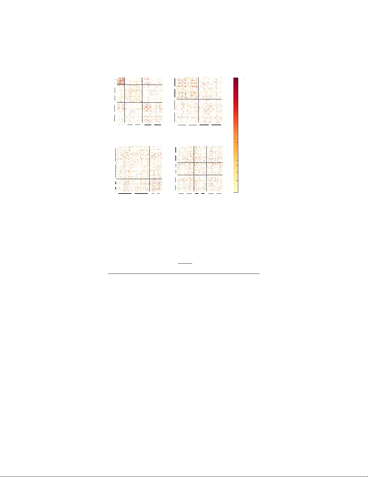
Net w ork mo dularit y in the presence of co v ariates Beate F rank e 1 P atrick J. W olfe 1 , 2 1 Departmen t of Statistical Science, Universit y College London 2 Departmen t of Computer Science, Universit y College London Abstract W e c haracterize the large-sample properties of net work mo dularit y in the presence of co v ariates, under a natural and flexible nonparametric n ull mo del. This provides for the first time an ob jectiv e measure of whether or not a particular v alue of modularity is meaningful. In particular, our results quantify the strength of the relation b et ween observed communit y structure and the in teractions in a netw ork. Our technical con tribution is to pro vide limit theorems for mo dularit y when a comm unity assign- men t is giv en by no dal features or cov ariates. These theorems hold for a broad class of netw ork mo dels ov er a range of sparsity regimes, as well as weigh ted, multi-edge, and pow er-law net works. This allows us to as- sign p -v alues to observed comm unity structure, which w e v alidate using sev eral b enc hmark examples in the literature. W e conclude by applying this metho dology to in vestigate a multi-edge netw ork of corporate email in teractions. Key w ords: cen tral limit theorems, degree-based net work mo dels, net- w ork communit y structure, nonparametric statistics, statistical netw ork analysis A fundamen tal c hallenge in mo dern science is to understand and explain net- w ork structure: in particular, the tendency of no des in a netw ork to connect in c ommunities based on shared c haracteristics or function. Scientists inevitably observ e not only netw ork nodes and their connections, but also additional in- formation in the form of cov ariates. Most analysis metho ds fail to exploit this information when attempting to explain net work structure, and instead assign comm unities based solely on the netw ork itself. This leads to a loss of in ter- pretabilit y and presen ts a barrier to understanding. W e solv e this problem, by sho wing how to decide whether communities defined b y cov ariates lead to a v alid summary of netw ork structure. In the studen t friendship net work sho wn in Fig. 1, for example, this means we can ev aluate whether communities based on common gender, race, or year in sc ho ol can explain the observed structure of the friendships. The strength of comm unity structure in net w orks is most often measured b y modularity [1], which is intuitiv e and practically effectiv e but until now has lac ked a sound theoretical basis. W e derive mo dularity from first principles, 1 giv e it a formal statistical in terpretation, and show why it w orks in practice. Moreo ver, by ac knowledging that differen t communit y assignments may explain differen t aspects of a net work’s observ ed structure, w e extend the applicability of mo dularit y beyond its typical use to find a single “best” communit y assignmen t. W e use co v ariates to define comm unity assignments, and then pro ve that mo dularit y quan tifies how well these cov ariates explain netw ork structure. W e sho w a fundamen tal limit theorem for mo dularit y in this context: in the pres- ence of cov ariates, it behav es like a Normal random v ariable for large netw orks whenev er there is a lac k of comm unit y structure. This allows us to translate mo dularit y into a probability (a p -v alue), enabling for the first time its use to dra w defensible, rep eatable conclusions from netw ork analysis. Our main tec hnical contribution is a flexible, nonparametric approach to quan tify the strength of observ ed communit y structure. Most work assumes a single unobserve d or laten t comm unity assignment (e.g., sto c hastic block mo dels [2] and laten t space models [3]). Hoff et al. [3] and Zhang et al. [4] both estimate laten t communit y structure, while adjusting for the v arying effects of cov ariates. F osdick and Hoff [5] simultaneously mo del cov ariates and latent structure, pro- viding a test for independence. In con trast, we deriv e limit theorems to ev aluate observe d comm unity structure implied by the cov ariates themselves. The existing statistical literature on mo dularity has fo cused on more basic parametric approaches. F or example, the authors of [6] and [7] model all edges as equally likely Bernoulli random v ariables. In contrast, we take a nonparametric approac h: using a single parameter per node, w e model only the exp ectation of eac h edge [8]. This allo ws for individual no de-specific differences but av oids sp ecific distributional assumptions on the edges. Our results apply to a broad class of net work models, allo wing us to treat (among others) p o w er-law net works, w eighted net works, and those with m ultiple edges. 1 Net w ork mo dularit y in the presence of co v ari- ates Tw o essential ingredients are necessary to understand modularity in the pres- ence of cov ariates: first, a framework to allow for a formal interpretation of mo dularit y as a measure of statistical significance; and second, the use of this framew ork to ev aluate a cov ariate-based communit y assignment. W e no w de- scrib e each of these ingredien ts in turn. First, to interpret mo dularit y as a measure of statistical significance, w e m ust recognize it as an estimator of a p opulation quan tity . Let g ( · ) denote an assignmen t of nodes into groups (i.e., communities), and write δ g ( i )= g ( j ) = 1 when no des i and j are assigned to the same group, and 0 otherwise. Denote by A ij the strength of an edge (e.g., a count or a weigh t) b et ween nodes i and j , and by d i = P j 6 = i A ij the degree of the i th node. Then, mo dularit y as defined 2 (a) Race (b) Y ear in school (c) Gender (d) Randomized Figure 1: A student friendship net work illustrated for four different communit y assignmen ts, eac h defined b y a cov ariate [5, 9]. in [1] is b Q = n X j =1 X i 0 : E A ij = π i π j , 1 ≤ i < j ≤ n. F urthermor e, c onsidering a se quenc e of such networks as n gr ows, we assume they ar e wel l b ehave d asymptotic al ly: 1. No single no de dominates the network: max i π i / ¯ π , with ¯ π = 1 n P n l =1 π l , is b ounde d asymptotic al ly; 2. The network is not to o sp arse: min i π i · √ n diver ges as n gr ows; 3. The exp e ctation of e ach e dge E A ij do es not diver ge to o quickly as n gr ows: max i π i / √ n go es to 0; 4. The varianc e of e ach e dge do es not vary to o much fr om its exp e ctation: V ar A ij / E A ij is b ounde d fr om ab ove and away fr om 0 asymptotic al ly; and 5. The skewness of e ach e dge A ij is c ontr ol le d: the thir d c entr al moment E h ( A ij − E A ij ) 3 i divide d by the varianc e V ar A ij is b ounde d asymptoti- c al ly. W e make no further assumptions on the distribution of A ij , and so our results apply in man y settings, including weigh ted netw orks and those with m ultiple edges. Assumptions 1 – 3 are structural: the first excludes star-lik e net- w orks; the second ensures that the netw ork is not to o sparse; and the third con trols the growth of E A ij with n in the w eighted or multi-edge setting. As- sumptions 4 and 5 are tec hnical; they exclude extreme b eha vior of the edge v ariables. F or instance, both are fulfilled whenev er A ij ∼ Bernoulli( π i π j ) or A ij ∼ P oisson( π i π j ). Eac h parameter π i describ es the relative p opularity of node i . Th us, to fit the degree-based mo del of Definition 1 to a net w ork, we estimate the parameters π i using the no de’s degrees d i as follows [8, 10, 11]: ˆ π i = d i p P n l =1 d l , 1 ≤ i ≤ n. (3) The estimator ˆ π i is b oth more natural and more computationally efficient than the corresp onding maximum-lik eliho od estimator for π i , whic h follo ws from the theory of generalized linear mo dels and cannot b e written explicitly in closed form. In many settings the difference b et ween these estimators is prov ably small [10], and so prop erties of maximum likelihoo d estimation can also be exp ected to hold for Eq. (3). Most imp ortan tly , w e show that any finite collection of estimators defined b y Eq. (3) tends to ward a multiv ariate Normal distribution when n is large and Definition 1 is in force. This generalizes a univ ariate result in [11] which assumes Bernoulli( π i π j ) edges and a p o wer law degree distribution. 5 Theorem 2 (Multiv ariate central limit theorem for Eq. (3)) . Assume the mo del of Definition 1 and any finite set of estimators fr om Eq. (3) . R elab eling the indic es of these estimators fr om 1 to r without loss of gener ality, we have that as n → ∞ , v u u t n X l =1 E d l ˆ π 1 − π 1 √ V ar d 1 , . . . , ˆ π r − π r √ V ar d r d → Normal(0 , I r ) . F urthermor e, p n V ar d i / P n l =1 E d l is b ounde d asymptotic al ly, and c an b e c on- sistently estimate d if A ij ∼ Bernoulli( π i π j ) or Poisson( π i π j ) by substituting ˆ π for π in V ar d i and E d i . F rom Definition 1 and Eq. (3), it is natural to define d E A ij = ˆ π i ˆ π j = d i d j P n l =1 d l , 1 ≤ i < j ≤ n. Substituting d E A ij for E A ij in Eq. (2), w e immediately recognize mo dularit y b Q as defined in Eq. (1). Thus, mo dularit y implicitly assumes the degree-based mo del of Definition 1. Moreo ver, d E A ij − E A ij con verges in probability to zero under the mo del of Definition 1 (see App endices). As a consequence of Theorem 2, w e then obtain a central limit theorem for d E A ij . Corollary . As n → ∞ under the mo del of Definition 1, d E A ij − E A ij q π 2 j V ar d i + π 2 i V ar d j / P n l =1 E d l d → Normal(0 , 1) . F urthermor e, q [ n/ E A ij ] · π 2 j V ar d i + π 2 i V ar d j / P n l =1 E d l is b ounde d asymp- totic al ly, and c an b e c onsistently estimate d if A ij ∼ Bernoulli( π i π j ) or A ij ∼ P oisson( π i π j ) by substituting ˆ π for π . This result leads to the first of tw o key insights as to why mo dularit y , when appropriately shifted and scaled, b eha ves lik e a Normal(0 , 1) random v ariable. Recall that b Q (Eq. (1)) is an estimator for its p opulation coun terpart Q (Eq. (2)), in whic h d E A ij estimates E A ij . Comparing Eqs. (1) and (2), and appro ximating d E A ij b y E d i d j / P n l =1 E d l , we obtain: E ( b Q − Q ) ≈ n X j =1 X i=100 lega | {z } legal trading d | {z } trading trading der | {z } others (a) By departmen t lega | {z } legal trading d | {z } trading trading der | {z } others 1 2 3 4 5 10 50 >=100 male genderi | {z } senior traditional exi | {z } junior (b) By seniorit y male genderi | {z } senior traditional exi | {z } junior hello ech o he 1 2 3 4 5 10 50 >=100 male gender hahah | {z } male traditi | {z } female (c) By gender male gender hahah | {z } male traditi | {z } female h 1 2 3 4 5 10 50 >=100 legaltradi | {z } A-H trading | {z } I-Q trading a | {z } R-Z (d) By last name initial legaltradi | {z } A-H trading | {z } I-Q trading a | {z } R-Z 1 2 3 4 5 10 50 >= 100 ≥ Figure 3: Multi-edges A ij in the Enron corp orate email dataset (153 emplo y ees, 32261 pairwise email exchanges), group ed according to four different cov ariate- based communit y assignments. Shading indicates the num b er of emails ex- c hanged. Co v ariate (no. groups) b Q − ˆ b p -v alue ˆ s Eq. (6) Bo otstrap Departmen t (3) 6 . 17 < 10 − 6 < 10 − 6 Seniorit y (3) 3 . 14 9 × 10 − 4 8 × 10 − 6 Gender (2) 2 . 36 9 × 10 − 3 2 × 10 − 3 First name initial (17) 0 . 74 2 × 10 − 1 2 × 10 − 1 Last name initial (3) − 0 . 46 7 × 10 − 1 7 × 10 − 1 T able 2: Analysis of the data of Fig. 3, using mo dularity deriv ed from multiple co v ariate-based communit y assignments. P oisson( π i π j ), NegativeBinomial( π i π j , r ) with common shap e parameter r , and zero-inflated versions of both. Figure 4 shows how well these distributions model the m ulti-edges. Even without zero-inflation, the negativ e Binomial distribution yields a go od fit, particularly in the righ t tail. A formal mo del comparison via suitable likelihoo d ratio tests [19] confirms this: as T able 3 shows, the negative Binomial achiev es the b est balance b etw een fitting the observ ed data (residual 11 Histogram f or model comparison f or Enr on data Edge v alue Edge count 0 1 2 4 7 19 49 125 315 793 1994 0 1 10 100 1000 10000 Data P oisson Zero−infl P oisson Negativ eBinomial Multi-edge v alue Number of occurrences Co v er upp er Co v e r lo w ert Data Poisson Zero-inflated P oisson Negative Binomial (NB) and zero-inflated NB Histogram f or model comparison f or Enr on data Edge v alue Edge count 0 1 2 4 7 12 19 31 49 78 199 500 1258 3161 0 1 10 100 1000 10000 Data P oisson Zero−infl P oisson Negativ eBinomial Histogram f or model comparison f or Enr on data Edge v alue Edge count 0 1 2 4 7 12 19 31 49 78 199 500 1258 3161 0 1 10 100 1000 10000 Data P oisson Zero−infl P oisson Negativ eBinomial Histogram f or model comparison f or Enr on data Edge v alue Edge count 0 1 2 4 7 12 19 31 49 78 199 500 1258 3161 0 1 10 100 1000 10000 Data P oisson Zero−infl P oisson Negativ eBinomial Histogram f or model comparison f or Enr on data Edge v alue Edge count 0 1 2 4 7 19 49 125 315 793 1994 0 1 10 100 1000 10000 Data P oisson Zero−infl P oisson Negativ eBinomial Histogram f or model comparison f or Enr on data Edge v alue Edge count 0 1 2 4 7 19 49 125 315 793 1994 0 1 10 100 1000 10000 Data P oisson Zero−infl P oisson Negativ eBinomial Histogram f or model comparison f or Enr on data Edge v alue Edge count 0 1 2 4 7 19 49 125 315 793 1994 0 1 10 100 1000 10000 Data P oisson Zero−infl P oisson Negativ eBinomial Figure 4: Observ ed versus exp ected email counts for maximum-lik elihoo d fits of four different mo dels satisfying Definition 1. Mo del for the Degrees Residual Relativ e m ulti-edges A ij of freedom deviance change P oisson 153 142031 − 39% Zero-inflated Poisson 154 57070 − 37% Negativ e Binomial (NB) 154 12671 − 19% Zero-inflated NB 155 12671 0% T able 3: Goo dness-of-fit v ersus model complexit y for the mo dels in Fig. 4 (start- ing from the 1-parameter mo del Poisson( λ ), relativ e to a saturated negative Binomial mo del with r → ∞ ). deviance) and mo del complexity (degrees of freedom). W e th us choose the mo del A ij ∼ Negativ eBinomial( π i π j , r ) . (7) Step 2: T o verify the assumptions of Definition 1 for our data, w e first as- sess Assumptions 1 and 2 exactly as b efore. Computing quartiles Q 1 – Q 3 of the degrees—68 , 200 , 564—we see that Q 3 /Q 2 and Q 1 / √ Q 2 are b oth of order one. Assumption 3 (max i π i / √ n shrinking) can b e analogously assessed via Q 3 / ( n √ Q 2 ). Assumptions 4 and 5 require V ar A ij / E A ij = 1 + π i π j /r and E h ( A ij − E A ij ) 3 i / V ar A ij = 1 + 2 π i π j /r to b e bounded. T o assess this, w e observ e that a maxim um-lik eliho o d estimate of r [19] yields ˆ r = 0 . 047, while the first three quartiles of d E A ij are resp ectiv ely 0 . 16 , 0 . 59 , 2 . 1. Step 3: T o estimate b and s in Theorem 1, we substitute ˆ π i for π i in Eqs. (4) and (5) exactly as b efore. Recall, ho wev er, that to estimate s w e also require an 12 estimate of V ar A ij in Eq. (5). Under the parametrization of Eq. (7), it follows that V ar A ij = π i π j (1 + π i π j /r ) . (8) Th us, V ar A ij can b e estimated b y substituting ˆ π i for π i and ˆ r for r in (8). This yields the required estimators ˆ b and ˆ s . Step 4: T o calculate p -v alues, we m ust first compute ( b Q − ˆ b ) / ˆ s for each co v ariate. In adv ance of our analysis, we would exp ect that employ ee gender, seniorit y , and departmen t might reflect aspects of communit y structure in email in teractions. In contrast, w e would expect co v ariates based on the first or last name of each individual to b e non-informativ e. Figure 3 illustrates, in decreasing order of ( b Q − ˆ b ) / ˆ s , the observed structure of our data when grouped b y cov ariate. T able 2 rep orts tw o appro ximate p -v alues per cov ariate, in contrast to the previous section. The first of these derives (via Eq. (6)) from Theorem 1, which sho ws the limiting distribution of ( b Q − ˆ b ) / ˆ s under the assumed model to b e a standard Normal. The second is based on 10 7 replicates of the parametric b ootstrap, whereby we fit a negativ e Binomial mo del to the data and then sim ulate from the fitted v alues to obtain an empirical finite-sample distribution. T able 2 indicates that our asymptotic theory is somewhat conserv ative in this setting, leading as it do es here to larger p -v alues than the b o otstrap. Finally , considering these p -v alues in more detail, we see from T able 2 that for the cov ariates of departmen t, gender, and seniorit y , all p -v alues fall b elo w 1% (leading to a corrected total of 5% after adjusting for multiple comparisons). In contrast, we obtain large p -v alues for first- and last-name co v ariates. This matc hes our exp ectations that department, gender, and seniorit y are likely to ha ve an impact on email interactions, while there is no obvious reason wh y this should hold for name-related cov ariates. 7 Discussion Net works ha ve ric her and more v aried structure than can be describ ed b y a single “b est” comm unit y assignment. T o reflect this, we ha v e introduced an approac h which exploits the structural information captured b y co v ariates, each of which may describ e different asp ects of comm unity structure in the data. In con trast to communit y dete ction p er se, this approac h allows us to assess the significance of a given, interpretable communit y assignment with resp ect to the observ ed netw ork structure. As describ ed in the data analysis examples ab ov e, our metho d leads to the iden tification of structurally significant communit y assignmen ts, ultimately yielding a b etter understanding of the netw ork under study . In tec hnical terms, w e hav e established a cen tral limit theorem for mo dularity under a nonparametric null mo del, yielding p -v alues to assess the significance of observ ed communit y structure. The mo del w e introduce shows explicitly how mo dularit y measures v ariabilit y in the data that cannot b e explained solely b y no de-sp ecific prop ensities for connection. What is more, mo dularit y has 13 more explanatory p o wer than a classical (chi-squared) go o dness-of-fit statistic: b y aggregating the estimated signe d residuals A ij − d i d j / P l d l within ev ery net work communit y , it measures the global tendency of a giv en communit y assignmen t to explain the observ ed netw ork structure. T o adv ance the state of the art in netw ork analysis, we as a research com- m unity must use this explanatory p o wer to understand the effects of multiple observ ed communities on net work structure. Our work here represen ts a first step in this direction: we use the explanatory p o wer of modularity to assess the significance of observed communit y structure relative to a null mo del. This op ens the door to more adv anced uses of multiple observ ed communit y assign- men ts within formal statistical mo deling frameworks. This is an imp ortant next step, since we see clear evidence here that m ultiple groupings ma y explain differen t aspects of a netw ork’s communit y structure. Ac kno wledgmen ts The authors thank Dr. Leon Danon for sharing the data on jazz musicians from [13] and Mar ´ ıa Dolores Alfaro Cuev as for pro ducing Fig. 2. This work was supp orted in part by the US Army Researc h Office under Multidisciplinary Uni- v ersity Research Initiative Award 58153-MA-MUR; b y the US Office of Na v al Researc h under Aw ard N00014-14-1-0819; b y the UK Engineering and Physi- cal Sciences Research Council under Mathematical Sciences Established Career F ellowship EP/K005413/1; b y the UK Ro yal So ciet y under a W olfson Research Merit Aw ard; and by Marie Curie FP7 Integration Gran t PCIG12-GA-2012- 334622 within the 7th Europ ean Union F ramework Program. A Notation and assumptions F or the follo wing pro ofs we will alwa ys consider an undirected random graph on n no des with no self-lo ops. W e mo del the edges A ij as indep enden t random v ariables with exp ectation E A ij = π i π j , A ij ≥ 0; 1 ≤ i < j ≤ n where π = ( π 1 , . . . , π n ) ∈ R n > 0 . W e will denote the degree of no de i as d i ; i.e., d i = P j 6 = i A ij . The remaining five assumptions of Definition 1 of the degree- based mo del are not all needed at all times and will therefore b e men tioned explicitly . F or conv enience we restate the assumptions below, all of whic h ref- erence a sequence of netw orks where n → ∞ . 1. No no de dominates the net work; i.e, n max i π i / k π k 1 = O (1); 2. The netw ork is not to o sparse; i.e., min i π i = ω (1 / √ n ); 3. The exp ectation of each edge do es not div erge to o quickly; i.e., max i π i = o ( √ n ); 14 4. The ratio of v ariance to expectation of each edge is controlled; i.e., ∀ i, j : V ar A ij / E A ij = Θ(1); and 5. The skewness of each edge A ij is controlled; i.e., ∀ i, j : E h ( A ij − E A ij ) 3 i / V ar( A ij ) = O (1). W e use bold letters to denote v ectors. B Pro of of Theorem 2 W e first show a univ ariate central limit theorem for the scalar estimator ˆ π i = d i / p k d k 1 . W e then extend this result to the multiv ariate case, applying the Cram ´ er–W old theorem. Preliminaries: Since the edges A ij , i < j are independent, it follo ws as sho wn in [11] that for finite n E d i = π i ( k π k 1 − π i ) , (9) V ar d i = X i 6 = j V ar A ij , (10) co v ( d i , d j ) = ( V ar A ij , i 6 = j V ar d i , i = j (11) E k d k 1 = k π k 2 1 − k π k 2 2 , (12) V ar k d k 1 = 2 n X i =1 V ar d i . (13) Theorem B.1 (Central limit theorem for ˆ π i ) . Consider Assumptions 1 – 5. De- fine ˆ π i = d i / p k d k 1 as an estimator of π i . Then as n → ∞ , ˆ π i − π i p V ar d i / E k d k 1 d → Normal(0 , 1) . F urthermor e, p V ar d i / E k d k 1 = O (1 / √ n ) , and c an b e c onsistently estimate d using a plug-in estimator for A ij ∼ Bernoulli( π i π j ) and A ij ∼ P oisson( π i π j ) . Pr o of. The pro of is a generalization of the pro of of Theorem 3.2 in [11], whic h assumes Bernoulli edges and a p o wer la w degree distribution. W e write ˆ π i − π i p V ar d i / E k d k 1 = d i − E d i √ V ar d i | {z } T 1 + E d i − π i p k d k 1 √ V ar d i | {z } T 2 s E k d k 1 k d k 1 | {z } T 3 . (14) 15 T o deduce the required result, we show that T 1 con verges in distribution to a Normal(0 , 1) random v ariable and T 2 and T 3 go in probability to 0 and 1, re- sp ectiv ely . Slutsky’s theorem enables us to combine the results and to obtain the claimed conv ergence in distribution. T erm T 1 : Each degree d i = P j 6 = i A ij is a sum of indep enden t random v ariables. F rom Assumption 2 ( ⇒ E d i → ∞ ) and Assumption 4 ( E A ij = Θ(V ar A ij )), it follo ws that V ar d i → ∞ . Since in addition, the skewness of eac h edge A ij is asymptotically b ounded (Assumption 5), the Lyapuno v condi- tion for exp onent 1 is satisfied; i.e., P j 6 = i E h ( A ij − E A ij ) 3 i h P j 6 = i V ar A ij i 3 / 2 → 0 . Hence, the Lindeberg–F eller Central Limit Theorem allows us to conclude that T 1 d → Normal(0 , 1). T erm T 2 : W e write T 2 = E d i − π i p k d k 1 √ V ar d i = E d i − π i p E k d k 1 √ V ar d i | {z } a ) − π i p k d k 1 − π i p E k d k 1 √ V ar d i | {z } b ) . (15) T erm T 2 con verges in probability to 0 since b oth a) the first ratio con verges to 0 and b) the second ratio con verges to 0 in probability . a) This conv ergence is driven by the fact that E d i − π i p E k d k 1 = O (1) (see Eqs. (9) and (12)) while V ar d i → ∞ . More precisely , E d i − π i p E k d k 1 √ V ar d i = π i k π k 1 1 − q 1 − k π k 2 2 / k π k 2 1 − π 2 i √ V ar d i . (16) Considering ˜ π = π / max j π j , we can conclude from k ˜ π k 2 2 ≤ k ˜ π k 1 that k π k 2 2 k π k 2 1 = (max j π j ) 2 k ˜ π k 2 2 (max j π j ) 2 k ˜ π k 2 1 ≤ 1 k ˜ π k 1 = max j π j k π k 1 . (17) Assumption 1 implies that max j π j / k π k 1 = O (1 /n ), and th us w e conclude k π k 2 2 k π k 2 1 = O 1 n . (18) 16 This allows us to apply a con vergen t T aylor expansion of √ 1 − x at 0 in Eq. (16): E d i − π i p E k d k 1 √ V ar d i (19) = π i k π k 1 h 1 − 1 − k π k 2 2 / 2 k π k 2 1 + o k π k 2 2 / k π k 2 1 i − π 2 i √ V ar d i = π i h k π k 2 2 / 2 k π k 1 + o k π k 2 2 / k π k 1 i − π 2 i √ V ar d i ≤ π i [max j π j / 2 + o (max j π j )] − π 2 i √ V ar d i (see Eq. (17)) = Θ π i (max j π j − π i ) √ E d i (Assumption 4) = Θ √ π i (max j π j − π i ) p k π k 1 − π i ! = O max j π j − π i √ n . (Assumption 1) Since π j = o ( √ n ) for all j (Assumption 3), it follows that the left-hand side of Eq. (19) conv erges to 0 in n . b) W e show b elo w that the second ratio π i p k d k 1 − π i p E k d k 1 / √ V ar d i in Eq. (15) con verges in probability to 0; this follows since π i / √ V ar d i → 0 un- der Assumptions 1 and 4 (see c) b elo w) and p k d k 1 − p E k d k 1 = O P (1) (see Lemma B.1 b elow). c) F rom Assumption 4 it follo ws that π i √ V ar d i = Θ π i √ E d i = Θ r π i k π k 1 − π i = O 1 / √ n . (Assumption 1) (20) Lemma B.1. Consider Assumptions 2 – 5. Then, p k d k 1 − p E k d k 1 = O P (1) . Pr o of. Observe that the square root function has one con tinuous deriv ative at 1. A T a ylor expansion in probability of p k d k 1 / E k d k 1 ab out 1 requires in addition [20, p. 201] that I. ∃ a ∈ R : k d k 1 / E k d k 1 = a + O P ( r n ); with I I. r n → 0 as n → ∞ . I. It follows from Chebyshev’s inequality that k d k 1 / E k d k 1 = 1 + O P p V ar k d k 1 / E k d k 1 . (21) 17 I I. As a consequence of I., r n = p V ar k d k 1 / E k d k 1 . F rom Eq. (12) and Assumption 2 ( ⇒ E d i → ∞ ) it follows that E k d k 1 → ∞ . Since A ij are inde- p enden t for i < j , and since we assume V ar A ij / E A ij = Θ(1) (Assumption 4), it holds that V ar k d k 1 E k d k 1 = V ar 2 P n j =1 P i 0 ) 46 Condition 2: P n j =1 P i
Original Paper
Loading high-quality paper...
Comments & Academic Discussion
Loading comments...
Leave a Comment