A Bayesian baseline for belief in uncommon events

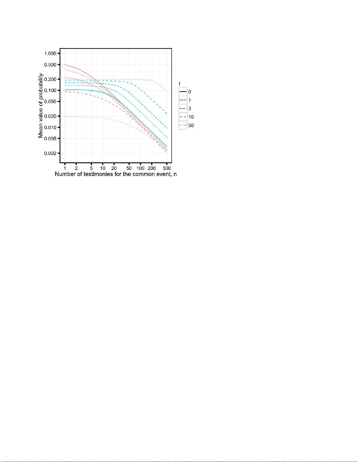
A B a y e s i a n b a s e l i n e f o r b e l i e f i n u n c o m m o n e v e n t s V. Palonen Department of Ph ysics, University of Helsinki, P.O. Box 43, 00014 University of Helsinki, Finland vesa.palonen@helsinki.fi ABSTRACT The plausibility of uncommon events and miracles based on testimony of such an event has been much discussed. When analyzin g the proba bilities involv ed, it has mostly been a ssumed that the common events can be taken as data in the calculations. However, we usually have o nl y testimonies for the common events. While this difference does not have a significant effect on the inductive part of the inference, it has a large influence on how one should view the r eliability of testi monies. In this work, a full Bayesian solution is given for the more realistic case, where one has a large number of testimonie s fo r a common event and one testimon y for an uncommon event. It is seen that, in order for there to be a large amount of testimonies for a common event, the testimonies will probably be quite reliable. For this reason, because the testimonies are quite reliable based on the testimonies for the common e vents, the probabilit y for the uncommon event, given a tes timony for it, is also higher. Hen ce, one should be m ore open-minded when c onsidering the plausibility of uncommon events. INTR ODUCTION Is it reasonable to believe in a testimony of an unco mmon event in the face of uniform co ntrary evidence from prior events? This question has been much discussed histo rically, with no table contributions from David Hume (Hume 1748) , John Ear man (Earman 200 0) , Millican (Millican 2013), and many others. David Hume’s argu ment was not clearly formulated, but Hume basically argued that the evidenc e for common events is so strong that the testimony f or uncomm on events (miracles) is usually not strong en ough e vidence fo r the uncommon event to be believable. “Extraordinary claims r equire extraordinary evidence” is the oft - us ed and dangerously po orly- defined phrase often connec ted to Hume’s position. Earman does a systematic job of both trying to find a precise form for Hume’s arg ument and then showing the problems there of. Earman makes two imp ortant points: 1. With a Bayesian calculation o f inducti ve inference, the probability of an unco mmon event d oes indeed go down with the amount of co mmon events (as 1/(n+2)), but never t o zero. Hence, based on induction, one can hence nev er be certain that the unc ommon won’t happe n. 2. Earman discusses the role and reliability of testimoni es for uncommon events. Earman shows that the testimony can often provide enough credibility for the uncommon event. Notably, in considering the evidential force of a testimony, one needs to consider, not just how often witnesses are wro ng in general, but what is th e probability that the wi tness would ma ke just such a particular cla im and be in error wi th that clai m. For ex ample, when a witness is testifying that John Doe won the lotte ry, it is not enough to suggest that a testimony is in general wrong with e.g. 10% probability, but one needs to take into account the pr obability that the claim was made abo ut John Doe in particular (why just him?) and also what is the probability tha t the claim indeed would be e rroneous. Presently the calculations published on the topic assume a lar ge am ount of com mon event s. In reality we u sually only have a large a mount of testimonies for the common events. That is, we do not have a unifor m evidence against the uncommon events. What we may have is uniform testimony against the uncommon events or miracles. In this sense it can be said that up to now the problem of uncommon events and their believa bility based on testim ony has not been fully analyz ed even on the basic level. This paper offers a full Bayesian so lution for the more realistic case, namel y, for the question: How believabl e is an uncom mon event when we have a uniform mass of testimony t o the contrary? The calculati on can b e seen as a baseline for further discussions o n the to pic, with nuances to be added as later as different additions and changes to the mo del are ex plored. Further co nsid eration will involve considera tions for several testi monies o f the same event, the independence of the witnesses, the effects of prior beliefs against the uncomm on event, and whether or n ot those testifying to a rare event are less trustworthy than th ose t estifying to a common event. a further complication in th e field has been that the usage o f probabilities in the discussion has been partial, with several authors dissecting the full f ormulas for partial arguments based on the full formulati on, see e.g. (Ahmed 2015), with the full solution nowhere to be seen. The aim her e will be to show the full s olution for the sim ple default situation with f ew assumptions. From there, different assumptions can be added whenever the assumptions are w ell grounded. The calculation will be made for a general case f or which we have te stim onies of com mon events and one testimony of an unc ommon event. The results will the n apply to miracles, t estimonies of rare natural events like winning a lotter y, and rare-event measurem ents in physics (e.g. pro ton decay). NOMENCLATURE Below is a tab le of notations used in the paper. For simplicit y, the logical and symbol  is usually dr opped in the probability notati on.  Not A    A and B    A or B 󰇛 󰇜 Conditional probability of A being true gi ven that B is true 󰇛 󰇜 Probability of A and B. W An uncommon event (whit e ball drawn from an urn) B A common event (bla ck ball drawn for an urn )   The result of the i ’th event is common ( i ’th ball was black) t(…) Testimony of an event n Number of testi monies of a common ev ent  󰇛  󰇜  n testimonies of a common event   A vector of n real events (W or B) behi nd the n testimonies v The (unknown) pr obability for the unco mmon event to happen d The (unknown) probability for a testimony to be wrong,        󰇛  󰇜   󰇛  󰇛  󰇜 󰇜 . THE BASELI NE MO DEL Using the above n otation, th e simple general case is this: Th ere are n te stimonies t of a common event B ,  󰇛  󰇜  and one testimony for an uncommon event W , 󰇛 󰇜 . What is the probability of W being in fact true given the testimonies,  󰇛     󰇛  󰇜  󰇛  󰇜  󰇜 ? We will assume as little as we can about the reliabilit y of t he witnesses (d) and about the real probabilit y o f the uncommon event happening (v). In effect, we will assign only reasonable prior probabilities for these probabilities and in the end let the data decide the most probable valu e s for the se probabilities. (These kinds of priors are often call ed hyperpriors in the dat a-analysis literature.) For si mplicity, we will use unif orm priors   󰇛   󰇜    󰇛   󰇜  where the notation   󰇛   󰇜 means that the probability density for x is co nstant betwee n a and b and zero elsewhere. With the latter prior we have assumed that in general the testimo nies are over 80% reliable, an assumption which will be seen to mat ter less and less as n increases. We will be using general Bayesian methodology, which is basically finding out the joint probability distribution for all the parameters relevant to the case and calculating the wanted probability distribution from the joint distribution by using marginali zation and the Bay es rule. (This approach is generally applicable and much used in the machine-learning community because from the joint distribution one can systematically calculate what ever probability one happens to need.) In this case, the joint distribution factors as (see App endix A for details)  󰇛     󰇛  󰇜  󰇛󰇜     󰇜   󰇛  󰇜  󰇛  󰇜  󰇛    󰇜 󰇛     󰇜  󰇛  󰇛  󰇜     󰇜 󰇛 󰇛 󰇜     󰇜 And the wanted probabil ity is  󰇛     󰇛  󰇜  󰇛  󰇜  󰇜  󰇛  󰇛  󰇜  󰇛  󰇜  󰇜 󰇛 󰇛  󰇜  󰇛  󰇜  󰇜  󰇛  󰇛  󰇜  󰇛  󰇜  󰇜  󰇛   󰇛  󰇜  󰇛  󰇜  󰇜  󰇛  󰇛  󰇜  󰇛  󰇜  󰇜          where we have ter ms of the form (by marginali zation)     󰇛   󰇛  󰇜  󰇛  󰇜  󰇜        󰇛     󰇛  󰇜  󰇛  󰇜   󰇜       where the sum is over all possible combinations o f the ele ments o f   , that is, we m arginali ze over all the possibilities in 󰇛     󰇜  󰇛     󰇜      󰇛     󰇜 . After calculations, the ter m s amoun t to (see the Appendix A for details)        󰇛    󰇜󰇛         󰇜      and        󰇛    󰇜   󰇛         󰇜      With these ter ms in hand, we are now in the position to show some result s. Re sult s of the ba seli ne mo del To reiterate, in previous works (see e.g. (Earman 2000)), it has been shown that when n common events are taken as data, simple Bayes ian inference with reas onable priors as signs a 1/( n +2) probability for the unc ommon event happening. This simple case of inductive inference does not take into account the te stim onies fo r the events (common or unc ommon), as is done in the current model. Figure 1 shows the probability for the uncommon event, with one testimony for the uncomm on event, as a function o f n , the number of te stimonies for the c ommon event,  󰇛     󰇛  󰇜  󰇛  󰇜  󰇜 . Perhaps surprisingly, as the number of testimonies for t he comm on event ( n ) grows large, the probab ility f or t he uncom mon e vent given the testimonies app roaches the valu e 0.5 asymptoticall y. There is a very larg e differen ce to the resul ts of the si mple inductive inference mentioned above, where the pr obability approaches ze ro asymptoticall y . Figure 1. Probability for the uncommon event in the face of n testimonies for a common event. Note the logarithmic horizontal axis. What is the reas on for the difference of the results for the pr esent more realistic model? Why does even one testimony for an uncomm on event overcome the inductive part of the inference from the large amount o f common events? The basic reason is that, for there to be a large consistent amount of te stim onies for the common events, the testimonies thems elves have to b e reliable. That is, if the testimoni es were unreliable, it would be un likely to have a unifor m set of testimonies for the co mmon ca se. R ather, there would likely be so me te stim onies for the uncommon event. On the other hand, if there are some past t estimonies f or the uncomm on event, the inductive part of the inference w ill not be so str ong against the uncommon events. Figure 2 sho ws the mean values of the probability of the uncommon event hap pening ( v ) and of the probability of a testimony being false ( d ). It is seen that as the number of testimonies ( n ) for the common event increases, the probability of the uncommon event decreases as expected, but at the same time the probability of a false testim ony also decreas es, and roughly at the same rate. Hence, even one testim ony for an uncommon event is able to balance out the inductive part of the inference and make the uncommon e vent believ able. Figure 2. Mean values for the probabilities for the uncommon event (red) and false testimony (blue ). Note the logarithmic axes. APPENDED CASE WITH KNOWN ER RONEOUS TESTIMONIE S Let us now append the previous case by including an l amount of false testi monies for the uncommon event. Our additional data is then     󰇛  󰇜  . The probabilit y we will be interest ed in is  󰇛     󰇛  󰇜  󰇛  󰇜     󰇛  󰇜  󰇜 . The joint distributi on will now factor as (se e Appendix B for more details)       󰇛  󰇜  󰇛  󰇜     󰇛  󰇜      󰇛  󰇜  󰇛  󰇜  󰇛    󰇜 󰇛     󰇜         󰇛  󰇛  󰇜     󰇜   󰇛  󰇜      󰇜 󰇛  󰇛  󰇜     󰇜 The calculations will p roceed as before, with some additional term. The wanted probability is again of the form  󰇛     󰇛  󰇜  󰇛  󰇜     󰇛  󰇜  󰇜             where         󰇛   󰇜  󰇛    󰇜   󰇛         󰇜              󰇛    󰇜     󰇛         󰇜      Re sult s fo r the ca se w ith e rron eo us t esti mo nies Figure 3 sho ws the probabil ity for the uncommon even t given the testimonies for the app ended case. Shown are cases with the numb er of known false testi monies l = 0, 1, 3, 10 , and 50. Figure 3. Prob ability for the u nc ommon even t in the face of n testimonies for a common e vent given different amounts of known false testimonies. Note the logarithmic hori zontal axis. Figure 4 shows the mean values o f the probabilities of the uncomm on event happening ( v ) and for a testimon y being false ( d ) for case s with different nu mber of known false tes timonies for the unco mmon event. Figure 4 . Mean values for the probabilities for the uncommon event ( re d) and false testimony (blue), given a number l of known false testimonies. Note the logarithmic axes. One can see from the results that a small a mount of known false testimonies for uncommon events do es not significantly alter the beli evability of an unc ommon event for which one testimony is not known to be false. For example, with three known false testimonies for an uncommon event and a large number of testimonies for common events, the probability for an unc ommon event given one t estimony for it is s till roughly 0.2. CONCLUSI ONS The main r esult of the p aper is that, when we have a l arge amount of testimonies for a com mon event and even only one testimony for a n uncommon event, the probability we should as sign for the uncommon event surprisingly larg e, namely 0.5. This is assuming that, without infor mation to the contrary, we are treating all the testimonies the same way, and we are not assuming additional structure (model comparison) for reality behind the events. This result has relevance for the study of miracles and also for science. In science, we should be more open to testimonies for “weird” empirical results which may not fit the current theoretical understanding. For example, Dr. Daniel Shechtman’s discovery of quasicr ystals (Sh echtman et al. 1984) shoul d have been met with more of an open mind by the community. In the case with some known-false te stim onies for the uncommon event, the probability for the uncommon event is lower but n ot sig nificantly so. Hence, the additional Humean argument against uncommon events based on some false t estimonies of uncommon e vents does not seem to have much force. It is noted that in the present model very few ass umptions wer e made and e.g. the probabilities for an uncommon event an d the testimonies were left o pen and decided bas ed on the available data. Yet, and importantly, it was assumed that the probabil ity of a f alse testimony is symmetric, that is, that it is as likely for a person to make a m istake in the testimony for an uncommon as in the testimony for a common event. Hence, the number of testi mo ni es for a common event had a bearing on the reliability on testimoni es in general and hence also for the testi mony for the uncommon event. It might be tempting to disconnect the two probabili ties or to assume that a t estimony for an unco mmon event is mor e likely to be false than a testimony for a co mmon event. While the former is possible, it would be hard to maintain that there is n o connection between the reliability for the testimonies of uncomm on and com mon events, the disconnection possibly leading to absurd results for low v alues o f n . The latter option of assuming that the testimonies for uncommon events are less reliable seems biased. Because such an assumption would equate bringing more in formation to bear on the ca se, there should be a clear and agreed -on grounding for making this assumption. The author suspects that such an assumption is n ot sustaina ble, but leaves that for fur ther, more nuanced, discus sions. For the model with known false testimonies for the uncomm on event , the false testim onies might be viewed as a reason to relax the symmetry of the reliability o f the testimoni es o f common and uncommon events. This exercis e and gr ounding thereof is also lef t for further study on the matter. REFE RENCES Ahmed, Arif. 2015. “Hume and the Independent Witnesses.” Mind 124 (496) (October 4): 1013 – 1044. doi:10.1093/mind /fzv076. Earman, john. 20 00. Hume’ s Abject Failure : The A rgument Against Miracl es . Oxf ord University Press, USA . Hume, David. 1748. An Enquiry Concerning Human Understanding . London: A. Millar. https://ebooks.adelaid e.edu.au/h/hume /david/h92e/. Millican, Peter. 2 0 13. “Earman on Hume on Mir acles.” In Debates in Modern Philosoph y: Essential Readings and Contemporary Respon ses , edited by Stewart Duncan and Antonia LoLord o. Routledge. Neapolitan, Richard E. 2004. Learning Bayesian Networks . Pearson Pren tice Hall. Pearl, Judea. 199 7. “Bayesian Networks. ” UCLA Co mputer Science Department, Technical Report R246: 1 – 5. Shechtman, D ., I. Blech, D . Gratias, and J. W. Cahn. 1984. “Metallic Phase with Long -Range Orientational Order and No Translational Symmetry.” Physical Review Letters 53 (20) (November 12): 1951 – 1953. doi:10.1103/Ph ysRevLett.53.1951. APPENDI X A DETAI LED C ALCULATI ONS FOR T HE BASEL INE MOD EL Joi nt fa cto riza tio n Figure A1 gi ves the dependencies b etween the para meters of the model as a directed acyclic graph (Pearl 1997; Neapolitan 2004 ). Figure A1. Directed acyclic graph of the case. The arrows in the graph represent dir ect probabilistic d ependencies between the parameters of the model. The natural factorization of the joint distributi on can be read from the DAG (Neapolit an 200 4) to be  󰇛     󰇛  󰇜  󰇛󰇜    󰇜   󰇛  󰇜  󰇛  󰇜  󰇛   󰇜 󰇛     󰇜  󰇛  󰇛  󰇜     󰇜 󰇛 󰇛 󰇜     󰇜 . Sum mati on ove r po ssi bil ities of C n Recall that in th e simple model we ha ve two terms of the for m     󰇛   󰇛  󰇜  󰇛  󰇜  󰇜        󰇛     󰇛  󰇜  󰇛  󰇜   󰇜       In this section we will calculate this ter m, notably the sum over all possibilities of   . Now          󰇛  󰇜  󰇛  󰇜  󰇛   󰇜 󰇛     󰇜  󰇛  󰇛  󰇜     󰇜 󰇛  󰇛  󰇜     󰇜            󰇛  󰇜  󰇛   󰇜     󰇛  󰇜  󰇛  󰇛  󰇜     󰇜    󰇛     󰇜  󰇛  󰇛  󰇜     󰇜            󰇛   󰇜     󰇛  󰇛  󰇜     󰇜        where the constan t c is a product of the c onstant priors of v and d , and  󰇛    󰇜    󰇛  󰇛  󰇜     󰇜          󰇛     󰇜  󰇛  󰇛  󰇜     󰇜    󰇛        󰇜  The following is an ind uctive proof for th e last identit y For S 2 , the sum is over the possibilities 󰇛     󰇜  󰇛     󰇜     󰇛        󰇜  󰇛  󰇛   󰇜  󰇛   󰇜        󰇜   󰇛        󰇜  󰇛  󰇛   󰇜  󰇛   󰇜        󰇜   󰇛        󰇜  󰇛  󰇛   󰇜  󰇛   󰇜        󰇜   󰇛        󰇜  󰇛  󰇛   󰇜  󰇛   󰇜        󰇜        󰇛    󰇜  󰇛    󰇜  󰇛    󰇜  󰇛  󰇜   󰇛        󰇜   Next, with a low er case c i we will deno te the i ’th element of C n and similarly f or  󰇛  󰇜  . For S n+1 , we have      󰇛     󰇜  󰇛  󰇛  󰇜     󰇜       󰇛       󰇜  󰇛  󰇛  󰇜  󰇛 󰇜       󰇜         󰇛     󰇜  󰇛     󰇜  󰇛  󰇛  󰇜     󰇜 󰇛 󰇛  󰇜    󰇜          󰇛     󰇜 󰇛 󰇛  󰇜    󰇜    󰇛        󰇜   APPENDI X B D ETAILED CALCULATI ONS FOR THE CA SE WIT H ERRONEOUS TEST IMONIES Figure B1 gives the dep endencies between th e parameters of the model. Figure B1. A directed acyclic graph of the model wi th er raneous testimoni es. Again, the joint distrib ution can be r ead from the graph to b e       󰇛  󰇜  󰇛  󰇜     󰇛  󰇜      󰇛  󰇜  󰇛  󰇜  󰇛    󰇜 󰇛     󰇜         󰇛  󰇛  󰇜     󰇜   󰇛  󰇜      󰇜 󰇛  󰇛  󰇜     󰇜 And the wanted probabil ity is  󰇛     󰇛  󰇜  󰇛  󰇜     󰇛  󰇜  󰇜   󰇛  󰇛  󰇜  󰇛  󰇜     󰇛  󰇜  󰇜 󰇛 󰇛  󰇜  󰇛  󰇜     󰇛  󰇜  󰇜             Where   󰆒             󰇛  󰇜  󰇛  󰇜     󰇛  󰇜              󰇛  󰇜  󰇛   󰇜           󰇛  󰇜  󰇛  󰇛  󰇜     󰇜   󰇛  󰇜      󰇜       󰇛     󰇜  󰇛  󰇛  󰇜     󰇜       󰇛   󰇜      󰇛    󰇜           And similarly   󰆒     󰇛   󰇜                