On short-term traffic flow forecasting and its reliability

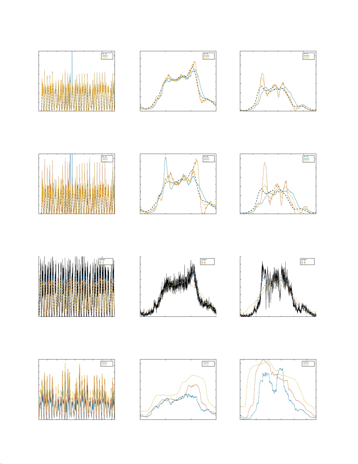
On short-term traffic flo w forecasting and its reliabilit y Hassane Ab ouaïssa ∗ Mic hel Fliess ∗∗ , ∗∗∗∗ Cédric Join ∗∗∗ , ∗∗∗∗ , † ∗ L ab or atoir e de Génie Informatique et d’A ut omatique de l’ Artoi s (LGI2A, EA 392 6), Université d’Artoi s, 62400 Béthune, F r anc e (e-mail: hassane.a b ouaissa@univ-artois.fr) ∗∗ LIX (CNRS, UMR 71 61), Éc ole p olyte chnique, 91128 Palaise au, F r anc e (e-mail : Michel. Fliess@p olyte chnique.e du) ∗∗∗ CRAN (CNRS, UMR 703 9), Université de L orr aine, BP 239, 54506 V andœuvr e-lès-Nancy, F r anc e (e-mail: c e dric.join@univ-lorr aine.fr) ∗∗∗∗ AL.I.E.N. (AL gèbr e p our Identific ation & Estimation Numériques), 24-30 rue Lio nnois, BP 60120, 54003 Nancy, F r anc e (e-mail: {michel. fliess, c e dric. join}@alien-sas. c om) † Pr ojet Non-A, INRIA Lil le – Nor d-Eur op e, F r anc e Abstract: Recent adv ances in time s e ries, wher e deterministic and sto chastic mo delings as well as the s torage and analysis o f big data a re useless, p ermit a new approach to short-ter m tr a ffic flow foreca sting and to its reliability , i. e. , to the traffic volatilit y . Sev eral con vincing co mputer simul ations, which utilize co ncrete data, are presented an d discussed. Keywor ds: Road tr affic, transp or tation control, manag ement systems, in telligent knowledge-based sys tems, time se r ies, foreca sts, per sistence, r is k, volatilit y , financia l engineering. 1. INTR ODUCTION W e recently prop osed a new feedback control la w for ramp metering (A b ouaïssa, Fliess, Iordanov a & Join (2012)), which is based on the most fruitful mo del-fr e e c ontr ol se t- ting (Fliess & J oin (2013)). It has no t only b een pa ten ted but also successfully tested in 20 15 on a highw ay in nor th- ern F ra nce. 1 It will so on b e implement ed on a lar ger scale. W e are therefore lead to s tudy another imp orta nt topic for in telligent transp ortation systems, i.e. , shor t-term traf- fic flo w forecasting: it plays a key rôle in the planning and development of traffic mana gement. This importa nce explains the ex tensiv e literature o n thi s sub ject since at least thirty years. Several surveys (se e , e.g. , Bolshinsky & F riedman (2012); Chang , Zhang, Y ao & Y ue (2011); Lippi, Bertini & F rasconi (2013); Smith, Williams & Oswald (2002); Vlaho gianni, K arlaftis & Go lias (2014 )) pr ovide useful informa tions on th e v a r ious appr oaches which have bee n a lready employ ed: regr ession ana ly s is, time s e ries, exp ert sys tems, artificial neural net works, fuzzy log ic, etc. W e follow here a nother r oad, i.e. , a new appro ach to time series (Fliess & Join (200 9 , 2015a,b); Fliess, Join & Ha tt (2011a ,b)): • A quite recent theor em due to Cartier & Perrin (1995) yields the most imp orta n t notions of tr en ds and quick fluctu ations , which do not s eem to ha ve any analog ue in other theoretical approaches. Among those existing appr oaches, the dominant one to day has been developed f or econometric g oals (se e , e.g. , 1 See, e.g. , the newspaper L a V oix du Nor d , 2 Decem b er 2015, p. 3 . Mélard (2008 ), T say (2010 ), and Meur io t (20 12) for some histo rical a nd epistemolog ical issues). It is quite po pular in traffic flow forecasting. • Although its orig in lies in financial engineering, it has bee n recen tly applied fo r sho rt-term meteoro logical forecasts for the purp ose of r enewable energ y man- agement (Join, V oy ant, Fliess, Nivet, Muselli, P aoli & Chaxel (2014 ); V oy a n t, Jo in, Fliess, Niv et, Muselli & Paoli (201 5); Join, Fliess, V oy ant & Chaxel (201 6)). • Lik e in model-free control (Fliess & Join (2013)), no deterministic or probabilistic mathematical modeling is needed. Moreov er the stor age and analysis of bi g data is useless.Thos e facts op en new p ersp ectives to in telligent knowledge-based sys tems. The reliability of those computations sho uld nevertheless be exa mined, at least for a b etter risk understanding. This sub ject, which is cr ucial for any t yp e of appro a ch, has bee n muc h less studied (see, e.g. , Guo, Huang & Williams (2014); Laflamme & Ossenbruggen (2014); Zhang, Zhang & Haghani (2 014), a nd the refere nce s therein). This r is k may of course b e studied v ia the concept of volatility , which may b e found everywhere in fina nce (see, e.g. , T s ay (2010); Wilmott (2006)). The strong a ttac ks a g ainst the very concept of volatilit y seem to hav e b een ignored in the communit y studying in telligent transp orta tion systems. W e a re th us repro ducing the following quote from Fliess, Join & Hatt (2 0 11a). Wilmott (2 006) (chap. 49, p. 813 ) writes: Quite fr ankly, we do not know what volatility curr ent ly is, never mind what it may b e in the futur e . The lack moreov er of a ny precise mathematical definition leads to multiple wa ys for computing v olatility which are by no means equiv alent and might even be sometimes misleading (see, e.g. , Goldstein & T aleb (2007)). Our theoretica l formalism a nd the co rresp onding computer simulations will confirm wha t most practitioners a lready know. It is well expresse d by Gunn (200 9) (p. 49): V olatility is not only r eferring to some thing that fluctuates sharply up and down but is also r eferring to something that moves sharply in a sustaine d dir e ction . Let us stress that in econometrics and in financial engineering the notion of v olatility is usually examined via the r eturns of financial assets. This setting seems to b e p ointless in the context o f traffic flow. Defining the volatility directly from the time series (see also Fliess, Join & Hatt (2011b)) makes muc h more se ns e. Our viewp oint on time series is sketched in Section 2 . Sec- tion 3 inv estig ates th e fundamental notion of p ersistenc e . The forecasting techniques for the traffic flow on a F rench highw ay and the corr espo nding computer exp eriments are discussed in Section 4. Shor t concluding rema r ks ma y b e found in Section 5. 2. REVISITING TIME SE RIES 2.1 Time series via nonstandar d analysis T ake the time int erv al [0 , 1] ⊂ R and introduce as o ften in nonstandar d analysis (see, e.g. , (Lobry & Sari (20 08); Fliess & Jo in (2009 , 2 015a)), and some of the references therein, for bas ics in nonstandar d analysis ) for the in- finitesimal sa mpling T = { 0 = t 0 < t 1 < · · · < t ν = 1 } where t i +1 − t i , 0 ≤ i < ν , is infinitesimal , i.e. , “very small”. A time series X ( t ) is a function X : T → R . A time s eries X : T → R is said to b e quickly fluctuating , or oscil lating , if, and only if, the in tegral R A X d m is infinitesimal, i.e. , v ery small, for any appr e ciable interv al, i.e. , a n interv al which is neither very small nor very large. A ccording to a theorem due to Cartier & P errin (1995 ) the following additive decomp osition holds for any time series X , whic h satisfies a weak integrabilit y condition, X ( t ) = E ( X )( t ) + X fluctuati on ( t ) (1) where • the me an , or aver age , E ( X )( t ) is “quite smo o th.”, • X fluctuati on ( t ) is q uic kly fluctuating. The deco mpo sition (1) is unique up to an infinitesimal. 2.2 On the numeric al differ entiation of a noisy signal Let us star t with the first degree p olyno mial time function p 1 ( τ ) = a 0 + a 1 τ , τ ≥ 0 , a 0 , a 1 ∈ R . Rewrite thanks to classic opera tional calculus with resp ect to the v aria ble τ (see, e.g. , Y osida (1984 )) p 1 as P 1 = a 0 s + a 1 s 2 . Multiply bo th sides b y s 2 : s 2 P 1 = a 0 s + a 1 (2) T ake the deriv a tiv e of both sides with respect to s , whic h corresp onds in the time domain to the multiplication by − t : s 2 dP 1 ds + 2 sP 1 = a 0 (3) The co efficient s a 0 , a 1 are obtained via the triangula r sys- tem o f equa tions (2)-(3). W e get r id of the time deriv atives, i.e., o f sP 1 , s 2 P 1 , a nd s 2 dP 1 ds , by multi plying both sides o f Equations (2)-(3) b y s − n , n ≥ 2 . The corresp onding iter- ated time integrals are low pass filters which a ttenuate the corrupting noises (see Fliess (2006) for an ex planation). A quite short time window is sufficien t for obtaining accurate v alues o f a 0 , a 1 . Note that estimating a 0 yields the trend. The extension to p olynomial functions of higher degr ee is straightforward. F or deriv ative e s timates up to some finite or der of a given smoo th function f : [0 , + ∞ ) → R , take a suitable truncated T aylor expa ns ion around a given time instant t 0 , a nd apply the pr evious co mputations . Resetting and utilizing sliding time windows per mit to estimate deriv atives of v arious or der s at any sampled time instant. R emark 1. See (Fliess, Join & Sira -Ramírez (2008); Mb oup, Join & Fliess (2009); Sira-Ramírez, Gar cía-Ro dríguez, Cortès-Romer o & Luv ia no-Juáre z (201 4)) for more details. 2.3 F or e c asting Set the following foreca st X est ( t + ∆ T ) , w her e ∆ T > 0 is not to o “large”, X forecast ( t + ∆ T ) = E ( X )( t ) +  dE ( X )( t ) dt  e ∆ T (4) where E ( X )( t ) and h dE ( X )( t ) dt i e are estimated like a 0 and a 1 in Section 2.2 . Let us s tress that what we predict is the trend and not the quick fluctuations (see also Fliess & Join (2009); Fliess, Jo in & Hatt (2011 b); Join, V oy ant , Fliess, Niv et, Muselli, P aoli & Chaxel (2014); V oyan t, Join, Fliess, Niv et, Muselli & P aoli (20 15)). 2.4 V olatility Contrarily to our previo us approa ch via returns (Fliess, Join & Hatt (201 1a,b)), we use here the difference X ( t ) − E ( X )( t ) b et ween the time series and its trend. If this difference is s quare int egrable, i.e. , if ( X ( t ) − E ( X )( t )) 2 is in tegrable, volatility is defined via the following s ta ndard deviation type form ula: v o l ( X )( t ) = q E ( X − E ( X )) 2 ≃ p E ( X 2 ) − E ( X ) 2 3. PERSISTE NCE 3.1 Definition The p ersistenc e metho d is the simplest way of pro ducing a forec ast. It assumes that the conditions at the time of the for e c ast will not c ha nge, i.e. , X forecast ( t + ∆ T ) = X ( t ) (5) 3.2 Sc ale d Persistenc e Sc ale d p ersisten c e , whic h is often encountered in meteorol- ogy (see, e.g. , (Lauret, V oyan t, Soub dhari, David & Poggi (2015)), and (Join, V oy ant, Fliess, Nivet, Muselli, Paoli & Chaxel (20 14); V oyan t, J oin, Fliess, Niv et, Muselli & Paoli (2015))) improves F o rmula (5) b y writing X Pe ( t + ∆ T ) = E ( X )( t ) × S c ( t ) (6) where • E ( X )( t ) is estimated like a 0 in Section 2.1, • the scaling factor S c ( t ) will be ma de precise according to the situation, • cont rarily to (5) quick fluctuations are disrega rded and the trend is emphasized. 4. CASE STUDY 4.1 Description Consider a section of the highw ay A25 from Dunkirk ( Dunker que in F rench) to Lille (see Fig ure 1). There ar e t wo lanes o n this s e ction, and ab out 90 0 m b etw een t wo measurements stations. C o ngestions often o ccur. The traf- fic volume, the o c c upa tion rate and and the mean v ehicle sp e ed, which yield excellent tra ffic characterizations, ar e measured. W e fo cus here on the traffic v olume Q ( t ) , in veh/min. It is reg is tered every min ute from 1 to 30 June 2014, a nd display ed in Fig ure 2-(a). T wo single days are detailed in Figures 2-(b) and 2-(c). I n all those Figur e s the trend is also dr awn. It is computed by using 10 0 p oints and the following non-ca usal moving average mean ( Q ( t − 49) , ..., Q ( t + 50)) = Q ( t − 49) + · · · + Q ( t + 50) 100 (7) 4.2 F or e c astings Let us emphasize that forecas ting er r ors will b e defined with resp ect to the trend derived from (7). Three foreca st horizons are considered : 5 , 1 5 , and 60 minutes. Set X ( t ) = Q ( t ) . The term E ( Q )( t ) in (4) and (6) are deduced fro m the ca us al moving av er a ge E 100 ( Q )( t ) = mean ( Q ( t − 99) , .. ., Q ( t )) = Q ( t − 99) + · · · + Q ( t ) 100 The scaling factor S c ( t ) in (6) is given b y S c ( t ) = E 100 ( Q )( t − 1 day + ∆ T ) E 100 ( Q )( t − 1 day ) where • 1day = 60 × 24 = 1 440 minutes, • ∆ T is equa l to one o f the three following v a lues : 5, 15, 6 0 minutes. Then (4) and (6) become r esp e ctiv ely Q A ( t + ∆ T ) = E 100 ( Q )( t ) +  dE 100 ( Q )( t ) dt  e ∆ T (8) and Q Pe ( t + ∆ T ) = E 100 ( Q )( t ) × E 100 ( Q )( t − 1 day + ∆ T ) E 100 ( Q )( t − 1 day ) (9) Computer exp eriments show that (8) and (9 ) suffer re- sp e ctiv ely from ra ther lar g e ov ersho ots and undersho ots. In order to remedy this annoying fact wr ite (9) in the for m Q Pe ( t + ∆ t ) = E 100 ( Q )( t ) + E 100 ( Q )( t ) S c ( t ) − 1 ∆ t ∆ t It yields the following forecasting equa tio n Q MixedF ore cast ( t + ∆ t ) = E 100 ( Q )( t ) + ˜ a 1 ( t )∆ t (10) where ˜ a 1 is equal to (1) dE 100 ( Q )( t ) dt if its mo dule is smaller than the module of E 100 ( Q )( t ) S c ( t ) − 1 ∆ t , (2) E 100 ( Q )( t ) S c ( t ) − 1 ∆ t if not. 4.3 Computer Exp eriments Results are display ed in Figures 3, 4 and 5 . The sup eriority of the forecasting (10) is obvious. T able 1, with its squar ed error s , provide a quantified compar ison of the v arious approaches. T able 1. P Errors 2 Horizon Pe Al [gain in %] Mi [gain in %] t + 5 min 2.08e+06 1.01e+06 [105%] 8.75e+05 [137%] t + 15 min 2.64e+06 1.7335e+06 [52%] 1.23e+06 [114%] t + 60 min 1.15e+07 8.47e+06 [36%] 4.29e+06 [169%] 4.4 V olatility Figure 6 displays the v ario us trends, whic h are computed via the non-causal mean (7), for three time scales: 10 0 , 250 , or 500 minutes. Note that larger is the time s cale smo other is the trend. O n the other hand Figure 7 shows a v olatility increase. Due to a lack o f space, o nly forecasting v olatility via F o rmula (8) for a 15 minutes time hor izon is display ed in Figur e 8, where the middle v alue, i.e. , 250 minu tes, is utilized for ca lcula ting the trend. The results are rather go o d. 5. CONCLUSION Although encour a ging our preliminary results need not only to b e further developed but a lso to b e compar ed with other ex is ting approa ches. Let us emphasize that such compa risons bega n to be discussed for s hort-term meteorolog ical forecasts by Join, V oyan t, Fliess, Niv et, Muselli, Paoli & Chaxel (2014 ) a nd V oy ant, Join, Fliess, Niv et, Muselli & Paoli (2 015). Our metho ds were easier to implemen t and m uc h less demanding in ter ms of historical data. F or a deep er study of re lia bilit y and risk, s e e J oin, Fliess, V oy ant & Chaxel (201 6) where the notion of c onfi- denc e b ands may b e extended to traffic management in a straightforw ard wa y . A CKNOWLED GEMENTS The Cer ema ( C entr e d’études et d’exp ertise sur les risques, l’e nvir onnement, la mobilité et l’aménagement ) provided the author s with the necess ary data for the highw ay A25. This hig h wa y is managed by the DIRN ( D ir e ct ion I nter dép artemen tale des R outes Nor d ) via the ALLE- GRO ( A gglomér ation liLLoise Exploitation Gestion de la RO ute ) s y stem. REFEREN CES H. Ab o uaïssa, M. Fliess, V. Iorda nov a, C. Jo in. F reewa y ramp metering con trol made easy and efficient. 13th IF AC Symp. Contr ol T r ansp ortation Systems , Sofia, 2012. O nline: ht tps:/ /hal.a rchives-ouvertes.fr/hal-00711847/en/ E. Bolshinsky , R. F r iedman. T r affic flow for e c ast survey . T ech. Rep., Comput. Sci. Dept., T echnion, Haifa, 2012. Fig. 1 . Our high way section time (min) × 10 4 0.5 1 1.5 2 2.5 3 3.5 4 20 40 60 80 100 120 Measure Trend (a) F rom 1 to 30 June 2014 time (min) 8500 9000 9500 10000 10 20 30 40 50 60 70 80 Measure Trend (b) Zo om 1 time (min) × 10 4 2.64 2.66 2.68 2.7 2.72 2.74 2.76 20 40 60 80 100 120 Measure Trend (c) Zo om 2 Fig. 2 . Measures and tre nd time (min) × 10 4 0.5 1 1.5 2 2.5 3 3.5 4 20 40 60 80 100 120 Trend Pe Al Mi (a) The whole set of data time (min) 8500 9000 9500 10000 10 20 30 40 50 60 70 80 Trend Pe Al Mi (b) Zo om 1 time (min) × 10 4 2.64 2.66 2.68 2.7 2.72 2.74 2.76 20 40 60 80 100 120 Trend Pe Al Mi (c) Zo om 2 Fig. 3 . 5 minutes for e c a sts time (min) × 10 4 0.5 1 1.5 2 2.5 3 3.5 4 20 40 60 80 100 120 Trend Pe Al Mi (a) F rom 1 to 30 June 2014 time (min) 8500 9000 9500 10000 10 20 30 40 50 60 70 80 Trend Pe Al Mi (b) Zo om 1 time (min) × 10 4 2.64 2.66 2.68 2.7 2.72 2.74 2.76 20 40 60 80 100 120 Trend Pe Al Mi (c) Zo om 2 Fig. 4 . 15 min utes forecasts time (min) × 10 4 0.5 1 1.5 2 2.5 3 3.5 4 20 40 60 80 100 120 Trend Pe Al Mi (a) The whole set of data time (min) 8500 9000 9500 10000 10 20 30 40 50 60 70 80 Trend Pe Al Mi (b) Zo om 1 time (min) × 10 4 2.64 2.66 2.68 2.7 2.72 2.74 2.76 20 40 60 80 100 120 Trend Pe Al Mi (c) Zo om 2 Fig. 5 . 60 min utes forecasts time (min) × 10 4 0.5 1 1.5 2 2.5 3 3.5 4 10 20 30 40 50 60 70 80 Measure Trend100 Trend250 Trend500 (a) The whole set of data time (min) 8500 9000 9500 10000 10 20 30 40 50 60 70 80 Measure Trend100 Trend250 Trend500 (b) Zo om 1 time (min) × 10 4 2.64 2.66 2.68 2.7 2.72 2.74 10 20 30 40 50 60 70 80 Measure Trend100 Trend250 Trend500 (c) Zo om 2 Fig. 6 . T r end and time scales time (min) × 10 4 0.5 1 1.5 2 2.5 3 3.5 4 2 4 6 8 10 12 14 16 18 20 Vol100 Vol250 Vol500 (a) The whole set of data time (min) 8500 9000 9500 10000 2 4 6 8 10 12 14 Vol100 Vol250 Vol500 (b) Zo om 1 time (min) × 10 4 2.64 2.66 2.68 2.7 2.72 2.74 2 4 6 8 10 12 14 Vol100 Vol250 Vol500 (c) Zo om 2 Fig. 7 . V ola tilit y and time scales time (min) × 10 4 0.5 1 1.5 2 2.5 3 3.5 4 2 4 6 8 10 12 14 16 18 20 Vol250 Al (a) The whole set of data time (min) 8500 9000 9500 10000 2 4 6 8 10 12 14 Vol250 Al (b) Zo om 1 time (min) × 10 4 2.64 2.66 2.68 2.7 2.72 2.74 2 4 6 8 10 12 14 16 18 20 Vol250 Al (c) Zo om 2 Fig. 8 . F or casting volatilit y P . Cartier, Y. Perrin. Integration ov er finite sets. F. & M. Diener editors: N onst andar d Analysis in Pr actic e , pp. 195–2 04, Springer , 199 5. G. Chang, Y. Zhang, D. Y ao, Y. Y ue. A summar y of short- term tr a ffic flow forecasting metho ds. IC CTP , 2011. M. Fliess. Analys e non standard du bruit. C.R. A c ad. Sci. Paris Ser. I , 342 : 797–8 02, 20 0 6 M. Fliess, C. Join. A mathematical pro of of the existence of trends in fina ncial time series. In A. El Ja i, L. Afifi, E. Zerrik, editor s, Systems The ory: Mo deling, Analysis and Contr ol , 43 –62, Presses Univ ersitaires de P erpignan, 2009. O nline: ht tps : //ha l.arc hives-ouvertes.fr/inria-00352834/en/ M. Fliess, C. Join. Mo del-free co nt rol. Int. J. Contr ol , 86 : 2228– 2252, 20 13. M. Fliess, C. Join, T ow ards a new viewpoint o n causality for time series. ESAIM Pr o cS , 49 : 37–52, 2 015a. Online: https ://ha l.archives-ouvertes.fr/hal-00991942/en/ M. Fliess, C. Join, Seaso nalities and cycles in time series: A fres h lo ok with co mputer exp eriments. Paris Finan. Manag. Conf. , Paris, 2015b. O nline: https ://ha l.archives-ouvertes.fr/hal-01208171/en/ M. Fliess, C. Jo in, F. Hatt. V olatility made obser v able at last. 3 es J. Identif. Mo dél. Exp érim. , Douai, 2011 a. Online: https : //hal .archive s-ouvertes.fr/hal-00562488/en/ M. Fliess , C. Jo in, F. Hatt. A-t-o n vr aiment besoin d’un mo dèle pro babiliste en ingénier ie financière ? Conf. Mé dit. In gén. Sûr e Syst. Compl. , Agadir, 2 011b. Online: https : //hal.a rchives-ouvertes.fr/hal-00585152/en/ M. Fliess, C. Join, H. Sira-Ra mírez. Non- linea r estimatio n is easy . Int. J. Mo del ling Identif. Contr ol , 4 : 12 –27, 2 0 08. Online: https : //hal .archive s-ouvertes.fr/inria-00158855/en/ D.G. Goldstein, N.N. T aleb. W e don’t quite k now what we are ta lking ab out when we talk ab out volatility . J. Portfolio Manage. , 33: 84– 86, 200 7. M. Gunn. T r ading Re gime Analy sis . Wiley , 20 09. J. Guo, W. Huang , B.M. Williams. Adaptiv e K alman filter approach for sto chastic short-term tra ffic flow prediction and uncertaint y quantifications. T r ansp ort. R es. C , 43 : 50–64 , 20 14. C. Join, M. Fliess , C. V oy ant, F. Chaxel. So la r ener gy pro duction: Short-term for ecasting a nd ris k manage- men t. 8th IF AC Conf. Manufact. Mo del. Manag. Contr. , T royes, 201 6. Online: https ://ha l.archives-ouvertes.fr/hal-01272152/en/ C. Jo in, C. V oyan t, M. Fliess, M. Mus e lli, M.-L. Nivet, C. Paoli, F. Chaxel. Shor t-term sola r irradiance and irradiation foreca sts via differen t time ser ies techniques: A pre limina r y study . 3r d Int . Symp. Envir on. F riend ly Ener gy Appl. , Paris, 20 14. Online: https ://ha l.archives-ouvertes.fr/hal-01068569/en/ E.M. La flamme, P .J. Ossenbruggen. The effect of sto ch as- tic volatility in pr edicting highw ay breakdowns. Symp. 50 Y e ars T r affic Flow The ory , P ortland, 20 1 4. P . Lauret, C. V oyan t, T. Soubdhan, M. David, P . Poggi. A benchmarking of machine learning techniques for s o lar radiation forecas ting in an insular co nt ext. Solar Ener g. , 112 : 44 6–457 , 2015 . M. Lippi, M. Bertini, P . F rasconi. Short-ter m traffic flow forecasting: An e xper imen tal compariso n of time-series analysis and sup ervised learning. IEEE T r ans. Intel. T r ansp ort. Syst. , 1 4 : 871– 882, 2013 . C. Lo bry , T. Sa ri. Nonstandard analysis and representa- tion of realit y . In t . J. Co ntr ol , 81 : 519 –53, 2 008. M. Mb oup, C. Join, M. Fliess. Numerical differentiation with annihilators in no isy en vironment. Num. Algo. , 50 : 439–4 67, 20 09. G. Mélard. Métho des de pr évision à c ourt terme . Ellipses & Presses Univ ersitaires de Br uxelles, 20 08. V. Meuriot. Une histoir e des c onc epts des séries tem- p or el les . Harmattan–A cademia, 2012. H. Sira-Ramír ez, C. García -Ro dríguez, J. Co rtès-Romero, A. Luviano- Juárez, A lgebr aic Identific ation and Estima- tion Metho ds in F e e db ack Contr ol Systems . Wiley , 20 14. B.L. Smith, B.M. Williams , R.K . Osw ald. Comparison of parametric a nd no nparametric mo dels for traffic flo w forecasting. T r ansp ort. R es. C , 10 : 303–3 2 1, 2 002. R.S. T say . Analy sis of Financial Time Series (3rd ed.). Wiley , 2010. E.I. Vlahogianni, M.G. K arlaftis, J.C. Go lias. Short-term traffic forecas ting: Where we are and where we are g oing. T r ansp ort. R es. C , 43 : 3 –19, 20 14. C. V oy ant, C. J oin, M. Fliess, M.-L. Nivet, M. Muselli, & C. Paoli. On meteorolog ical foreca sts for energy management a nd large histo r ical data: A first look . R enew. Ener. Power Quality J. , 13, 2015. Online: https : //hal.a rchives-ouvertes.fr/hal-01093635/en/ P . Wilmott. Paul Wilmott on Q uantitative Financ e , 3 vol. (2nd ed.). Wiley , 200 6. K. Y osida. Op er ational Calculus (translated from the Japanese). Springer , 1984 . Y. Z hang, Y. Zha ng , A, Haghani. A h ybrid short-term traffic flow foreca sting metho d based on sp ectral anal- ysis and statistical v olatility mo del. T r ansp ort. R es. C , 43 : 6 5–78, 2014 .