Practical Riemannian Neural Networks

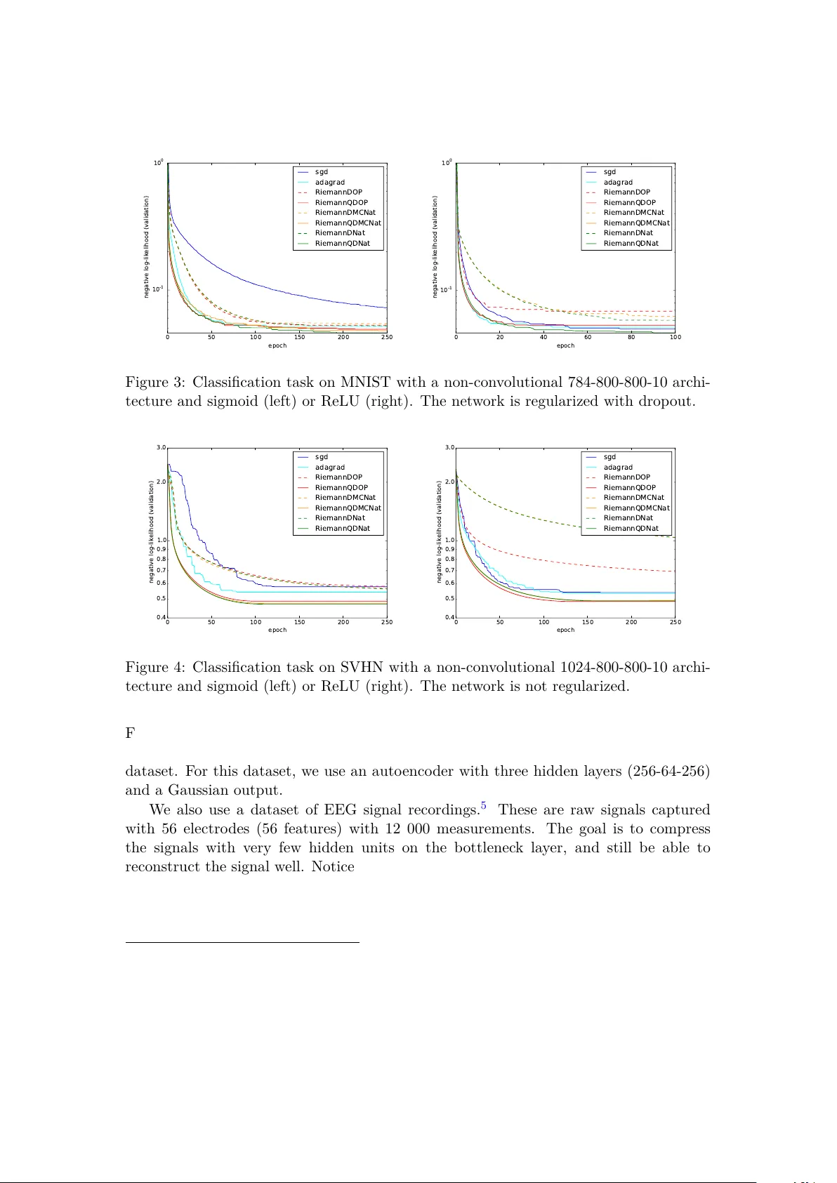
Practical Riemannian Neural Net w orks Gaétan Marceau-Caron Y ann Ollivier F ebruary 26, 2016 Abstract W e pro vide the first exp erimen tal results on non-syn thetic datasets for the quasi- diagonal Riemannian gradien t descents for neural netw orks introduced in [ Oll15 ]. These include the MNIST, SVHN, and F ACE datasets as well as a previously unpub- lished electro encephalogram dataset. The quasi-diagonal Riemannian algorithms consisten tly b eat simple sto c hastic gradien t gradien t descen ts b y a v arying margin. The computational ov erhead with resp ect to simple backpropagation is around a fac- tor 2 . P erhaps more interestingly , these metho ds also reac h their final performance quic kly , th us requiring few er training epo chs and a smaller total computation time. W e also presen t an implemen tation guide to these Riemannian gradien t descents for neural netw orks, showing how the quasi-diagonal v ersions can b e implemen ted with minimal effort on top of existing routines which compute gradients. W e presen t a practical and efficient implementation of inv ariant sto c hastic gradient descen t algorithms for neural netw orks based on the quasi-diagonal Riemannian metrics in tro duced in [ Oll15 ]. These can b e implemented from the same data as RMSProp- or A daGrad-based schemes [ DHS11 ], namely , by collecting gradients and squared gradien ts for each data sample. Th us we will try to present them in a wa y that can easily b e incorp orated on top of existing softw are providing gradien ts for neural netw orks. The main goal of these algorithms is to obtain in v ariance prop erties, suc h as, for a neural net work, insensitivit y of the training algorithm to whether a logistic or tanh acti- v ation function is used, or insensitivit y to simple c hanges of v ariables in the parameters, suc h as scaling some parameters. Neither backpropagation nor A daGrad-lik e sc hemes offer such properties. In v ariance prop erties are imp ortant as they reduce the num b er of arbitrary design c hoices, and guarantee that an observed goo d b ehavior in one instance will transfer to other cases when, e.g., different scalings are in volv ed. In some cases this ma y alleviate the burden associated to hyper-parameter tuning: in turn, sensible h yp er-parameter v alues sometimes b ecome inv arian t. P erhaps the most well-kno wn in v arian t training pro cedure for statistical learning is the natur al gr adient promoted by Amari [ Ama98 ]. Ho wev er, the natural gradient is rarely used in practice for training neural net works. The main reason is that the Fisher information metric on which it relies is computationnally hard to compute. Different appro ximations ha ve b een prop osed but can bring little b enefits compared to the im- plemen tation effort; see for instance [ RMB07 , Mar14 ]. Moreov er, it is not clear whether 1 these approximations preserve the inv ariance prop erties. 1 In the end, simpler tec hniques ha ve been prop osed to patch the fla ws of the plain sto chastic gradien t descent. Using a balanced initialization with rectified linear units, drop out and SGD or AdaGrad can b e enough to obtain very go o d results on many datasets. Nevertheless, these are tric ks of the trade, little justified from a mathematical p oint of view. The Riemannian framew ork for neural n et works [ Oll15 ] allows us to define several quasi-diagonal metrics, which exactly k eep some (but not all) inv ariance prop erties of the natural gradien t, at a smaller computational cost. The quasi-diagonal structure means that the gradient obtained at eac h step of the optimization is preconditioned b y the in verse of a matrix which is almost diagonal, with a few well-c hosen non-diagonal terms that make it easy to inv ert and hav e a special algebraic structure to ensure inv ariance with resp ect to some simple transformations such as c hanging from sigmoid to tanh activ ation function. In this rep ort, we assess the p erformance of these quasi-diagonal metrics (only tested on synthetic data in [ Oll15 ]). They turn out to b e quite comp etitive ev en after taking in to account their computational o verhead (a factor of ab out 2 with resp ect to simple bac kpropagation). These metho ds consistently impro ve p erformance by v arious amounts dep ending on the dataset, and also w ork well with drop out. Especially , con vergence is v ery fast early in the training pro cedure, which op ens the door to using fewer ep o chs and shorter ov erall training times. The co de used in the exp eriments is av ailable at https://www.lri.fr/~marceau/code/riemaNNv1.zip In v ariance and gradient descents. The simplest instance of parameter inv ariance is that of parameter scaling. Consider the classic gradien t step θ ← θ − η ∇ θ f (v anilla gradien t descent) (1) where ∇ θ f is the deriv ativ e of f w.r.t. θ . This iteration sc heme has an homogeneity problem in terms of physical units: the unit of the deriv ativ e ∇ θ f is the inv erse of the unit of θ . This means that the learning rate η itself should ha v e the homogeneit y of θ 2 for the gradient descen t ( 1 ) to b e homogeneous. This is one reason why sensible learning rates can change a lot from one problem to another. A daGrad-like metho ds [ DHS11 ] solv e one half of this problem by rescaling ∇ θ f b y its recen t magnitude, so that it b ecomes of order 1 (ph ysically dimensionless). The learning rate η then has the homogeneit y of θ , not θ 2 . This is particularly relev an t when it is kno wn in adv ance that relev ant parameter v alues for θ are of order 1 themselv es; if not, the learning rate η still needs to b e set to a v alue compatible with the order of magnitude of θ . Another example of lac k of inv ariance w ould b e a c hange of input enco ding. F or example, if a netw ork receiv es an image of a handwritten c haracter in black and white 1 F or instance, the rank-one approximation in [ RMB07 ] is defined in reference to the Euclidean norm of the difference betw een exact and approximated Fisher matrices, and thus, is not parameterization- indep enden t. 2 0 10 20 30 40 50 epoch 1 0 - 2 1 0 - 1 1 0 0 1 0 1 negative log-likelihood (test) normal pixels with step-size 0.1 inverted pixels with step-size 0.1 normal pixels with step-size 1.0 inverted pixels with step-size 1.0 Figure 1: Classification task on MNIST with a non-con volutional 784-100-10 architec- ture. The figure shows the impact of in v erting the pixels for t wo different step-sizes. or in white and black, or if the inputs are enco ded with 0 for black and 1 for white or the other w ay round, this is equiv alen t to changing the inputs x to 1 − x . A sigmoid unit with bias b and weigh ts w i reacts to x the same w ay as a sigmoid unit reacts to 1 − x if it has bias b 0 = b + P w i and w 0 i = − w i (indeed, b 0 + P w 0 i (1 − x i ) = b + P w i x i ). How ev er, the gradien t descent on ( b 0 , w 0 ) will b ehav e differen tly from the gradient descent on ( b, w ) , b ecause the corresp ondence mixes the weigh ts with the bias. This leads to p oten tially differen t performances dep ending on whether the inputs are white-on-black or black-on- white, as sho wn on Figure 1 . This sp ecific problem is solved by using a tanh activ ation instead of a sigmoid, but it w ould b e nice to hav e optimization pro cedures insensitiv e to suc h simple c hanges. Mathematically , the problem is that the gradient descent ( 1 ) for a differen tiable function f : E → R defined on an abstract vector space E , is only well-defined after a choice of (orthonormal) basis. Indeed, at eac h point θ of E , the differen tial ∂ f ∂ θ is a linear form (row v ector) taking a vector v as an argumen t and returning a scalar, ∂ f ∂ θ · v , the deriv ativ e of f in direction v at the current p oint θ . This differen tial is conv erted in to a (ro w) v ector by the definition of the gradien t: ∇ f is the unique vector such that ∂ f ∂ θ · v = h∇ f , v i for all vectors v ∈ E . This clearly dep ends on the definition of the inner pro duct h· , ·i . In an orthonormal basis, w e simply hav e ∇ f = ( ∂ f ∂ θ ) > . In a non-orthonormal basis, w e ha ve ∇ f = M − 1 ( ∂ f ∂ θ ) > where M is the symmetric, p ositive-definite matrix defining the inner pro d uct in this basis. Using the v anilla gradient descent ( 1 ) amoun ts to deciding that whatev er basis for θ w e are currently w orking in, this basis is orthonormal. F or tw o differen t parameteriza- tions of the same intrinsic quantit y , the v anilla gradient descen t pro duces t wo completely differen t trajectories, and may ev entually reac h different lo cal minima. As a striking ex- ample, if w e consider all points obtained with one gradien t step b y v arying the inner pro duct, we span the whole half-space where ∂ f ∂ θ · v > 0 . 3 Notice that an inner pro duct defines a norm k v k 2 : = h v , v i , which giv es the notion of length b etw een the p oin ts of E . The choice of the inner pro duct mak es it easier or more difficult for the gradient descent to mo ve in certain directions. Indeed the gradient descen t ( 1 ) is equiv alen t to θ ← θ + arg min δ θ { f ( θ + δ θ ) + k δ θ k 2 / 2 η } (2) up to O ( η 2 ) for small learning rates η : this is a minimization o ver f , p enalized by the norm of the up date. Th us the choice of norm k·k clearly influences the direction of the up date. In general, it is not easy to define a relev ant c hoice of inner pro duct h· , ·i if nothing is kno wn ab out the problem. Ho wev er, in statistical learning, it is p ossible to find a canonical choice of inner product that dep ends on the curr ent p oint θ . At each point θ , the inner pro duct b et ween tw o v ectors v , v 0 will b e h v , v 0 i θ = v > M ( θ ) v 0 , where M ( θ ) is a particular p ositive definite matrix depending on θ . Sev eral choices for h v , v 0 i θ are giv en b elow, with the prop erty that the scalar pro duct h v , v 0 i θ , and the asso ciated metric k v k θ , do not dep end on a c hoice of basis for the vector space E . (Note that the matrix M ( θ ) do es depend on the basis, since the expression of v and v 0 as vectors does.) The resulting R iemannian gradient tra jectory θ ← θ − η M ( θ ) − 1 ∂ f ∂ θ > (Riemannian gradient descen t) (3) is th us in v ariant to a c hange of basis in E . A ctually , when the learning rate η tends to 0 , the resulting con tinuous-time tra jectory is inv ariant to any smo oth homeomorphism of the space E , not only linear ones: this trajectory is defined on E seen as a “manifold” . Th us, the main idea b ehind in v ariance to co ordinate changes is to define an inner pro duct that do es not dep end on the n umerical v alues used to represen t the parameter θ . W e no w give several such constructions together with the asso ciated gradien t up date in volving M ( θ ) − 1 . In v arian t gradien t descen ts for neural netw orks. In mac hine learning, we hav e a training dataset D = ( x n , t n ) N n =1 where x n is a datum and t n is the associated target or lab el; w e will denote D x the set of all x n ’s in D , and lik ewise for D t . Supp ose that w e hav e a mo del, suc h as a neural net work, that for each input x pro duces an output y = y ( x, θ ) dep ending on some parameter θ to b e trained. W e supp ose that the outputs y are in terpreted as a probability distribution ov er the p ossible targets t . F or instance, in a classification task y will b e a v ector con taining the probabilities of the v arious p ossible lab els. In a regression task, we migh t assume that the actual target follows a normal distribution centered at the predicted v alue y , namely t n = y ( x n , θ ) + σ N (0 , Id) (in that case, σ may b e considered an additional parameter). Let p ( t | y ) b e the probabilit y distribution on the targets t defined by the output y of the netw ork. W e consider the log-loss function for input x and target t : ` ( t, x ) : = − ln p ( t | y ( x, θ )) (4) 4 F or instance, with a Gaussian model t = y ( x, θ ) + σ N (0 , Id) , this log-loss function is ( y − t ) 2 2 σ 2 + dim( y ) 2 ln(2 π σ 2 ) , namely , the square error ( y − t ) 2 up to a constan t. In this situation, there is a w ell-known choice of in v arian t scalar pro duct on parameter space θ , for whic h the matrix M ( θ ) is the Fisher information matrix on θ , M nat ( θ ) : = ˆ E x ∈D x E ˜ t ∼ p ( ·| y ) h ∂ θ ` ( ˜ t, x )( ∂ θ ` ( ˜ t, x )) > i (5) where ˆ E x ∈D x is the empirical a verage ov er the feature vectors of the dataset, and where ∂ θ ` ( ˜ t, x ) denotes the (column) vector of the deriv atives of the loss with resp ect to the parameter θ . F or neural net works the latter is computed b y backpropagation. Note that this expression inv olv es the losses on all p ossib le v alues of the targets ˜ t , not only the actual target for eac h data sample. The natur al gr adient is the corresp onding gradient descent ( 3 ), with f : = E ( x,t ) ∈D ` ( t, x ) the av erage loss ov er the dataset: θ ← θ − η M nat ( θ ) − 1 ∂ θ f (6) Ho wev er, the natural gradien t has several features that mak e it unsuitable for most large-scale learning tasks. Most of the literature on natural gradients for neural netw orks since Amari’s work [ Ama98 ] deals with these issues. First, the Fisher matrix is a full matrix of size dim( θ ) × dim( θ ) , whic h mak es it costly to inv ert if not imp ossible to store. Instead w e will use a low-storage, easily inv erted quasi-diagonal v ersion of these matrices, whic h k eeps many in v ariance prop erties of the full matrix. Second, the Fisher matrix inv olves an expectation ov er “pseudo-targets” ˜ t ∼ p ( ·| y ) dra wn from the distribution defined b y the output of the netw ork. This might not b e a problem for classification tasks for whic h the n umber of p ossibilities for t is small, but requires another approac h for a Gaussian mo del if w e w an t to a void n umerical in tegration o ver ˜ t ∼ y + σ N (0 , Id) . W e describ e three w ays around this: the outer pr o duct appro ximation, a Mon te Carlo approximation, or an exact v ersion whic h requires dim ( y ) bac kpropagations per sample. Third, the Fisher matrix for a giv en v alue of the parameter θ is a sum ov er x in the whole dataset. Th us, each natural gradient up date w ould need a whole sw eep ov er the dataset to compute the Fisher matrix for the current parameter. W e will use a mo ving a verage o ver x instead. Let us discuss eac h of these p oints in turn. Quasi-diagonal Riemannian metrics. Instead of the full Fisher matrix, we use the quasi-diagonal r e duction of M − 1 , whic h inv olv es computing and storing only the diagonal terms and a few off-diagonal terms of the matrix M . The quasi-diagonal reduction was in tro duced in [ Oll15 ] to exactly keep some of the inv ariance prop erties of the Fisher matrix, at a price close to that of diagonal matrices. Quasi-diagonal reduction uses a decomp osition of the parameter θ into blo cks. F or neural netw orks, these blo c ks will b e the parameters (bias and weigh ts) incoming to eac h 5 neuron, with the bias b eing the first parameter in each blo ck. In each blo ck, only the diagonal and the first row of the blo ck are stored. Thus the num b er of non-zero en tries to be stored is 2 dim ( θ ) (actually sligh tly less, since in each blo ck the first entry lies b oth on the diagonal and on the first row; in what follows, w e include it in the diagonal and alw ays ignore the first en try of the row). Main taining the first row in each block accoun ts for p ossible correlations b et ween biases and weigh ts, such as those appearing when the input v alues are transformed from x to 1 − x (see p. 3 ). This is why the bias plays a sp ecial role here and has to b e the first parameter in eac h blo c k. Quasi-diagonal metrics guarantee exact inv ariance to affine changes in the activ ations of each unit [ Oll15 , Section 2.3], including each input unit. The op erations w e will need to p erform on the matrix M are of tw o types: computing M by adding rank-one con tributions of the form v v > with v = ∂ θ ` ( ˜ t, x ) in ( 5 ), and applying the inv erse of M to a vector v in the parameter up date ( 3 ). F or quasi-diagonal matrices these op erations are explicited in Algorithms 2 and 1 . The cost is ab out twice that of using diagonal matrices. A b y-pro duct of this blo ck-wise quasi-diagonal structure is that eac h lay er can b e considered independently . This enables to implement the computation of the metric in a mo dular f ashion. F unction QDSolve( M , v ) Data : V ector v ; blo c k decomposition for the comp onents of v ; matrix M of size dim( v ) × dim ( v ) of which only the diagonal and the first row in eac h blo ck are known; regularization threshold ε > 0 . Result : Quasi-d iagonal inv erse QD( M ) − 1 .v foreac h blo ck of c omp onents of v do w ← k -th blo c k of v ; ∆ ← diagonal of the k -th blo c k of M ; r ← first ro w of the k -th blo c k of M ; ∆ ← ∆ + ε ; Index the comp on en ts of the blo ck from 0 to n k − 1 ; for i = 1 to n k − 1 (but NOT i = 0 ) do w i ← ∆ 0 w i − r i w 0 max ( ∆ i ∆ 0 − r 2 i , ε ) ; end w 0 ← 1 ∆ 0 ( w 0 − P n k − 1 i =1 r i w i ) ; Store w into the k -th blo c k of the result; end Algorithm 1: Pseudo-co de for quasi-diagonal inv ersion. The case when the first ro ws are ignored ( q = 0 ) corresponds to a diagonal in version diag( M + ε ) − 1 .v . In our exp eriments, ε is set to 10 − 8 . 6 F unction QDRankOneUpdate( M , v , α ) Data : V ector v ; blo c k decomposition for the comp onents of v ; matrix M of size dim( v ) × dim ( v ) of which only the diagonal and the first row in eac h blo ck are known; real n umber α . Result : Rank-on e up date M ← M + α. QD( v v > ) foreac h blo ck of c omp onents of v do w ← k -th blo c k of v ; ∆ ← diagonal of the k -th blo c k of M ; r ← first ro w of the k -th blo c k of M ; ∆ ← ∆ + α w  2 ; r ← r + α w 0 w > with w 0 the first entry of w ; Diagonal of the k -th blo ck of M ← ∆ ; First row of the k -th blo c k of M ← r ; end Algorithm 2: Pseudo-co de for quasi-diagonal accumulation: rank-one up date of a quasi-diagonal matrix. Online Riemannian gradien t descen t, and metric initialization. As the Fisher matrix for a given v alue of the parameter θ is a sum o ver x in the whole dataset, each natural gradient up date w ould need a whole sweep ov er the dataset to compute the Fisher matrix for the current parameter. This is suitable for batc h learning, but not for online sto chastic gradien t descent. This can b e alleviated by up dating the metric via a moving av erage M ← (1 − γ ) M + γ M minibatch (7) where γ is the metric update rate and where M minibatch is the metric computed on a small subset of the data, i.e., b y replacing the empirical av erage ˆ E x ∈D x with an empirical a verage ˆ E x ∈D 0 x o ver a minibatc h D 0 ⊂ D . T ypically D 0 is the same subset on which the gradien t of the loss is computed in a sto chastic gradien t sc heme. (This subset may be reduced to one sample.) This results in an online R iemannian gr adient desc ent . In practice, c ho osing γ ≈ 1 # minibatches ensures that the metric is mostly renew ed after one whole sw eep ov er the dataset. Usually we initialize the metric on the first minibatch ( γ = 1 for the first iteration), which is empirically b etter than using the identit y metric for the first up date. A t startup when using very small minibatc hes (e.g., minibatc hes of size 1 ) it ma y b e advisable to initialize the metric on a larger num b er of samples b efore the first parameter up date. (An alternative is to initialize the metric to Id , but this breaks inv ariance at startup.) Natural gradien t, outer pro duct, and Monte Carlo natural gradient. The Fisher matrix inv olv es an exp ectation ov er “pseudo-targets” ˜ t ∼ p ( ·| y ) drawn from the distribution defined b y the output of the netw ork: a backpropagation is needed for eac h p ossible v alue of ˜ t in order to compute ∂ θ ` ( ˜ t, x ) . This is acceptable only for classification 7 tasks for which the num b er of p ossibilities for t is small. Let us now describ e three wa ys around this issue. A first wa y to av oid the expectation ov er pseudo-targets ˜ t ∼ p ( ·| y ) is to only use the actual targets in the dataset. This defines the outer pr o duct approximation of the Fisher matrix M OP ( θ ) : = ˆ E ( x,t ) ∈D h ∂ θ ` ( ˜ t, x )( ∂ θ ` ( ˜ t, x )) > i (8) th us replacing ˆ E x ∈D x E ˜ t ∼ p ( ·| y ) with the empirical a verage ˆ E ( x,t ) ∈D . F or eac h training sample, we ha ve to compute a rank-one matrix given b y the outer pro duct of the gradien t for this sample, hence the name. This method has sometimes been used directly under the name “natural gradient”, although it has different prop erties, see discussion in [ PB13 ] and [ Oll15 ]. An adv antage is that it can b e computed directly from the gradient pro vided by usual bac kpropagation on each sample. The corresp onding pseudoco de is giv en in Algorithm 3 for a minibatch of size 1 . Data : Dataset D , a neural netw ork structure with parameters θ Result : optimized parameters θ while not finish do retriev e a data sample x and corresp onding target t from D ; forw ard x through the netw ork; compute loss ` ( t, x ) ; bac kpropagate and compute deriv ative of loss: v ← ∂ θ ` ( t, x ) ; up date quasi-diagonal metric using v v > : M ← (1 − γ ) M ; QDRankOneUpdate( M , v , γ ) ; apply inv erse metric: v ← QDSolve( M , v ) ; up date parameters: θ ← θ − η v ; end Algorithm 3: Online gradien t descen t using the quasi-diagonal outer pro duct metric. A second w ay to proceed is to replace the exp ectation ov er pseudo-targets ˜ t with a Mon te Carlo appro ximation using n M C samples: M M C nat ( θ ) : = E x ∈D x " 1 n M C n M C X i =1 ∂ θ ` ( ˜ t i , x )( ∂ θ ` ( ˜ t i , x )) > # (9) where eac h pseudo-target ˜ t i is dra wn from the distribution p ( ˜ t | y ) defined by the output of the netw ork for eac h input x . This is the Monte Carlo natur al gr adient [ Oll15 ]. W e ha ve found that n M C = 1 (one pseudo-target for each input x ) works w ell in practice. The corresp onding pseudo co de is given in Algorithm 4 for a minibatch of size 1 and n M C = 1 . 8 Data : Dataset D , a neural netw ork structure with parameters θ Result : optimized parameters θ while not finish do retriev e a data sample x and corresp onding target t from D ; forw ard x through the netw ork; compute loss ` ( t, x ) ; bac kpropagate and compute deriv ative of loss: v ← ∂ θ ` ( t, x ) ; generate pseudo-target ˜ t according to probabilit y distribution defined by the output lay er y of the net work: ˜ t ∼ p ( ·| y ) ; bac kpropagate and compute deriv ative of loss for ˜ t : ˜ v ← ∂ θ ` ( ˜ t, x ) ; up date quasi-diagonal metric using ˜ v ˜ v > : M ← (1 − γ ) M ; QDRankOneUpdate( M , ˜ v , γ ) ; apply inv erse metric: v ← QDSolve( M , v ) ; up date parameters: θ ← θ − η v ; end Algorithm 4: Online gradien t descent using the quasi-diagonal Monte Carlo nat- ural gradient, with n M C = 1 . The third option is to compute the exp ectation ov er ˜ t exactly using algebraic prop- erties of the Fisher matrix. This can b e done at the cost of dim ( y ) backpropagations p er sample instead of one. The details dep end on the t yp e of the output la yer, as follo ws. If the output is a softmax ov er K categories, one can just write out the exp ectation explicitly: M nat ( θ ) = ˆ E x ∈D x   K X ˜ t =1 p ( ˜ t | y ) ∂ θ ` ( ˜ t, x )( ∂ θ ` ( ˜ t, x )) >   (10) so that the metric is a sum of rank-one terms o ver all possible pseudo-targets ˜ t , w eighted b y their predicted probabilities. If the output mo del is multiv ariate Gaussian with diagonal co v ariance matrix Σ = diag( σ 2 k ) ( Σ may b e kno wn or learned), i.e., t = y + N (0 , Σ) , then one can pro ve that the Fisher matrix is equal to M nat ( θ ) = ˆ E x ∈D x " K X k =1 1 σ 2 k ∂ θ y k ( ∂ θ y k ) > # (11) where y k is the k -th comp onent of the netw ork output. The deriv ative ∂ θ y k can b e obtained by bac kpropagation if the backpropagation is initialized b y setting the k -th output unit to 1 and all other units to 0 . This has to b e done separately for eac h output unit k . Th us, for eac h input x the metric is a contribution of several rank-one terms ∂ θ y k ( ∂ θ y k ) > obtained by bac kpropagation, and w eighted b y 1 /σ 2 k . Another mo del for predicting binary data is the Bernoulli output, in whic h the ac- tivities of output units y k ∈ [ 0; 1] are interpreted as probabilities to hav e a 0 or a 1 . This 9 case is similar to the Gaussian case up to replacing 1 σ 2 k with 1 y k (1 − y k ) (in verse v ariance of the Bernoulli v ariable defined b y output unit k ). The pseudo co de for the quasi-diagonal natural gradien t is giv en in Algorithm 5 . Data : Dataset D , a neural net work structure with parameters θ , a quasi-diagonal metric M Result : optimized parameters θ while not finish do retriev e a data sample x and corresp onding target t from D ; forw ard x through the netw ork; compute loss ` ( t, x ) ; bac kpropagate and compute deriv ative of loss: v ← ∂ θ ` ( t, x ) ; M ← (1 − γ ) M ; Dep ending on output la yer in terpretation: Cate goric al output with classes {1,. . . ,K} : for e ach class ˜ t fr om 1 to K do Set ˜ t as the pseudo-target; α ← p ( ˜ t | y ) ; bac kpropagate and compute deriv ative of loss for ˜ t : ˜ v ← ∂ θ ` ( ˜ t, x ) ; up date quasi-diagonal metric using ˜ v ˜ v > : QDRankOneUpdate( M , ˜ v , γ α ) ; end Gaussian output (squar e loss) with varianc e diag( σ 2 k ) , k = 1 , . . . , K : for e ach output unit k fr om 1 to K do α ← 1 /σ 2 k ; ˜ v ← ∂ θ y k (obtained by setting bac kpropagated v alues on the k -th output unit to 1 , all the others to 0 , and bac kpropagating); up date quasi-diagonal metric using ˜ v ˜ v > : QDRankOneUpdate( M , ˜ v , γ α ) ; end apply inv erse metric: v ← QDSolve( M , v ) ; up date parameters: θ ← θ − η v ; end Algorithm 5: Online gradien t descen t using the quasi-diagonal natural gradient. Notably , the OP and Monte Carlo approximation b oth keep the inv ariance prop erties of the natural gradien t. This is not the case for other natural gradien t approximations suc h as the blo ckwise rank-one approximation used in [ RMB07 ]. Eac h of these approaches has its strengths and w eaknesses. The (quasi-diagonal) OP is easy to implemen t as it relies only on quantities (the gradien t for eac h sample) that ha ve b een computed an ywa y , while the Mon te Carlo and exact natural gradient must mak e bac kpropagation passes for other v alues of the output of the net work. 10 When the mo del fits the data well, the distribution p ( ˜ t | y ) gives high probability to the actual targets t and th us, the OP metric is a go o d approximation of the Fisher metric. Ho wev er, at startup, the mo del do es not fit the data and OP might p o orly appro ximate the Fisher metric. Similarly , if the output mo del is missp ecified, OP can p erform badly even in the last stages of optimization; for instance, OP fails miserably to optimize a quadratic function in the absence of noise, an example to k eep in mind. 2 The exact quasi-diagonal natural gradient is only affordable when the dimension of the output y of the netw ork is not to o large, as dim( y ) backpropagations p er sample are required. Th us the OP and Mon te Carlo approximations are app ealing when out- put dimensionalit y is large, as is t ypical for auto-enco ders. Ho wev er, in this case the probabilit y distribution p ( ˜ t | y ) is defined ov er a high-dimensional space, and the OP ap- pro ximation using the single deterministic p oint ˜ t = t ma y b e p o or. (In preliminary exp erimen ts from [ Oll15 ], the OP appro ximation p erformed p o orly for an auto-enco ding task.) On the other hand, Mon te Carlo integration often p erforms relatively w ell in high dimension, and migh t b e a sensible choice for large-dimensional outputs such as in auto-enco ders. Still, the choice b et ween these three options is largely exp erimental. Since all three ha ve closely related implementations (Algorithms 3 – 5 ), they can b e compared with little effort. Diagonal v ersions: F rom AdaGrad to OP , and in v ariance prop erties. The algorithms presen ted abov e with quasi-diagonal matrices also hav e a diagonal version, obtained by simply discarding the non-diagonal terms. (This breaks affine in v ariance.) F or instance, the up date for diagonal OP (DOP) reads M DO P ← (1 − γ ) M DO P + γ diag( ∂ θ ` ∂ θ ` > ) (12) where ∂ θ ` is the deriv ative of the loss ` for the curren t sample. This can b e rewritten on the vector of diagonal en tries of M DO P as diag( M DO P ) ← (1 − γ )diag( M DO P ) + γ ( ∂ θ ` )  2 (13) This up date is the same as the one used in the family of AdaGrad or RMSProp algo- rithms, except that the latter use the squar e r o ot of M in the final parameter up date: θ ← θ − η M − 1 / 2 Ada ∂ θ ` (14) 2 Indeed, suppose that the loss function is k θ − x k 2 / 2 σ 2 , corresponding to the log-loss of a Gaussian mo del with v ariance σ 2 , and that all the data p oints are x = 0 . Then the gradient of the loss is θ/σ 2 , the OP matrix is the square gradient θ 2 /σ 4 , and the OP gradient descen t is θ ← θ − η σ 2 /θ . This is muc h to o slow at startup and m uch to o fast for final conv ergence. On the other hand, the natural gradien t is θ ← θ − η θ whic h b ehav es nicely . The catastrophic b ehavior of OP for small θ reflects the fact that the data hav e v ariance 0 , not σ 2 . Its bad b ehavior for large θ reflects the fact that the data do not follow the mo del N ( θ , σ 2 ) at startup. In b oth cases, the OP approximation is unjustified hence a huge difference with the natural gradient. The Mon te Carlo natural gradien t will b ehav e better in this instance. This particular divergence of the OP gradient for θ close to 0 disappears as so on as there is some noise in the data. 11 where M Ada follo ws the same up date as M DO P . Thus, although AdaGrad shares a similar framew ork with DOP , it is not naturally in terpreted as a Riemannian metric on parameter space (there is no well-defined tra jectory on the parameter space seen as a manifold), b ecause taking the elemen t-wise square-ro ot breaks all p oten tial inv ariances. T o summarize, the diagonal v ersions DOP , DMCNat and DNat are exactly inv ariant to r esc aling of each parameter comp onen t. In addition, the quasi-diagonal versions of these algorithms are exactly inv arian t to an affine change in the activity of e ach unit , including the activities of input units; this co vers, for instance, using tanh instead of sigmoid, or using white-on-black instead of black-on-white inputs. In con trast, to our kno wledge AdaGrad has no inv ariance prop erties (the values of the gradients M − 1 / 2 Ada ∂ θ ` are scale-in v ariant in AdaGrad, but not the resulting parameter tra jectories, since the parameter θ is updated b y the same v alue whatev er its scale). Exp erimen tal studies. W e demonstrate the inv ariance and efficiency of Riemannian gradien t descen ts through exp erimen ts on a series of classification and regression tasks. F or eac h task, w e choose an arc hitecture and an activ ation function, and we p erform a grid search ov er v arious p o wers of 10 for the step-size. The step-size is kept fixed during optimization. Then, for each algorithm, we rep ort the curve asso ciated with the b est step size. The algorithms tested are standard sto chastic gradient descent (SGD), A daGrad, and the diagonal and quasi-diagonal v ersions of OP , of Monte Carlo natural gradien t (with only one sample), and of the exact natural gradien t when the dimension of the output la yer is not to o large to compute it. First, we study the classification task on MNIST [ LC ] and the Street View Hous- ing Num b ers (SVHN)[ NW C + 11 ]. W e work in a p ermutation-in v arian t setting, i.e., the net work is not conv olutional and the natural top ology of the image is not taken into accoun t in the netw ork structure. W e also con verted the SVHN images into grayscale images in order to reduce the dimensionalit y of the input. Note that these exp eriments are small-scale and not geared to wards obtaining state- of-the-art p erformance, but aim at comparing the b ehavior of sev eral algorithms on a common ground, with relativ ely small arc hitectures. 3 Exp erimen ts on the classification task confirm that Riemannian algorithms are b oth more inv ariant and more efficient than non-in v arian t algorithms. In the first exp erimen t w e train a net work with tw o hidden la yers and 800 hidden units p er lay er, without an y regularization, on MNIST; the results are giv en on Figure 2 . Quasi-diagonal algorithms (plain lines) conv erge faster than the other algorithms. Es- p ecially , they exhibit a steep slop e for the first few ep o chs, and quic kly reac h a satisfying p erformance. Their trajectories are also very similar for ev ery activ ation function. 4 The 3 In particular, w e hav e not used the test sets of these datasets, only v alidation sets extracted from the training sets. This is b ecause we did not wan t to use information from the test sets (e.g., hyperpa- rameters) b efore testing the Riemannian algorithms on other architectures, which will b e done in future w ork. 4 Note that their in v ariance prop erties guarantee a similar performance for sigmoid and tanh as they represen t equiv alent models using differen t v ariables, but not necessarily for ReLU which is a different mo del. 12 Algorithm mean (std) SGD 29.10 (0.76) A daGrad 33.39 (2.26) RiemannDOP 42.44 (1.26) RiemannQDOP 56.68 (3.75) RiemannDMCNat 58.17 (4.57) RiemannQDMCNat 68.01 (2.35) RiemannDNat 120.16 (0.34) RiemannQDNat 129.76 (0.34) T able 1: Computational time per ep o ch for a 784-800-800-10 architecture on MNIST with minibatch of size 500 on a CPU. tra jectories of SGD, AdaGrad, and the diagonally approximated Riemannian algorithms are more v ariable: for instance, SGD is close enough to the quasi-diagonal algorithms with ReLU activ ation but not with sigmoid or tanh, and A daGrad p erforms well with tanh but not with sigmoid or ReLU. Finally , the Mon te Carlo QD natural gr adient seems to b e a very go o d approximation of the exact QD natural gradient, even with only one Monte Carlo sample. This may be related to simplicity of the problem, since the probabilities of the output lay er conv erges rapidly to their optimal v alues. Quasi-diagonal algorithms are also efficien t in practice. Their computational cost is reasonably close to pure SGD, as shown on T able 1 , with an ov erhead of ab out 2 as could b e exp ected. They are often m uch faster to learn in terms of n umber of training examples pro cessed, compared to SGD or A daGrad. The quasi-diagonal algorithms also b ehav e well with the drop out regularization [ SHK + 14 ], as can b e seen on Figure 3 . Several runs wen t b elow 1% classification error with this simple 800-800, p ermutation-in v ariant architecture. Three groups of tra jec- tories are clearly visible on Figure 3 , with A daGrad fairly close to the quasi-diagonal algorithms on this example. There is a clear difference b et ween the quasi-diagonal algorithms and their diagonal appro ximations: keeping only the diagonal breaks the in- v ariance to affine transormations of the activities, whic h th us app ears as a key factor here as well as in almost all exp eriments b elo w. On a more difficult dataset, the p erm utation in v ariant SVHN with grayscale images, w e observe the same pattern as for the MNIST dataset, with the quasi-diagonal algo- rithms leading on SGD and AdaGrad (Figure 4 ). How ev er, ReLU is severely impacting the diagonal approximations of the Riemannian algorithms: they diverge for step-sizes larger than 10 − 5 . This emphasizes once more the imp ortance of the quasi-diagonal terms. W e also test the algorithm on a deep er architecture on the MNIST dataset, with the goal of testing whether Riemannian algorithms handle “v anishing gradients” [ Ho c91 ] b etter. W e use a sparse net work with a connectivity factor of 10 incoming w eights p er unit. The conn ection graph is built from the output to the input by randomly c ho osing, for eac h unit, ten units from the previous lay er. The last output lay er is fully connected. 13 0 5 10 15 20 25 epoch 1 0 - 2 1 0 - 1 1 0 0 1 0 1 negative log-likelihood (training) sgd adagrad RiemannDOP RiemannQDOP RiemannDMCNat RiemannQDMCNat RiemannDNat RiemannQDNat 0 5 10 15 20 25 epoch 1 0 - 1 1 0 0 negative log-likelihood (validation) sgd adagrad RiemannDOP RiemannQDOP RiemannDMCNat RiemannQDMCNat RiemannDNat RiemannQDNat 0 5 10 15 20 25 epoch 1 0 - 1 1 0 0 negative log-likelihood (validation) sgd adagrad RiemannDOP RiemannQDOP RiemannDMCNat RiemannQDMCNat RiemannDNat RiemannQDNat 0 5 10 15 20 25 epoch 1 0 - 1 1 0 0 negative log-likelihood (validation) sgd adagrad RiemannDOP RiemannQDOP RiemannDMCNat RiemannQDMCNat RiemannDNat RiemannQDNat Figure 2: Classification task on MNIST with a non-conv olutional 784-800-800-10 arc hi- tecture without regularization. W e use a s igmoid (upp er left and upp er right), a tanh (lo wer left) and a ReLU (lo wer righ t). W e c ho ose a netw ork with 8 hidden lay ers with the follo wing architecture: 2560-1280- 640-320-160-80-40-20. The n umber of parameters is relatively small (56310 parameters), and since the architecture is deep, this should b e a difficult problem already as a purely optimization task (i.e., already on the training set). F rom Figure 5 , w e observe three groups: SGD is v ery slo w to con verge, while the quasi-diagonal algorithms reach quite small loss v alues on the training set (around 10 − 4 or 10 − 5 ) and p erform reasonably w ell on the v alidation set. A daGrad and the diagonal approximations stand in b etw een. Once more, quasi-diagonal algorithms hav e a steep descent during the first epo chs. Note the v arious plateaus of several algorithms when they reach very small loss v alues; this ma y b e related to numerical issues for suc h small v alues, esp ecially as we used a fixed step size. Indeed, most of the plateaus are due to minor instabilities which cause small rises of the loss v alues. This may disapp ear with step sizes tending to 0 on a schedule. Next, w e ev aluate the Riemannian gradient descen ts on a regression task, namely , reconstruction of the inputs. W e use the MNIST dataset and the fac es in the wild dataset (F A CES) [ HJLM07 ], again in a p ermutation-in v ariant non-conv olutional setting. F or the 14 0 50 100 150 200 250 epoch 1 0 - 1 1 0 0 negative log-likelihood (validation) sgd adagrad RiemannDOP RiemannQDOP RiemannDMCNat RiemannQDMCNat RiemannDNat RiemannQDNat 0 20 40 60 80 100 epoch 1 0 - 1 1 0 0 negative log-likelihood (validation) sgd adagrad RiemannDOP RiemannQDOP RiemannDMCNat RiemannQDMCNat RiemannDNat RiemannQDNat Figure 3: Classification task on MNIST with a non-conv olutional 784-800-800-10 arc hi- tecture and sigmoid (left) or ReLU (righ t). The netw ork is regularized with drop out. 0 50 100 150 200 250 epoch 1.0 0.4 0.5 0.6 0.7 0.8 0.9 2.0 3.0 negative log-likelihood (validation) sgd adagrad RiemannDOP RiemannQDOP RiemannDMCNat RiemannQDMCNat RiemannDNat RiemannQDNat 0 50 100 150 200 250 epoch 1.0 0.4 0.5 0.6 0.7 0.8 0.9 2.0 3.0 negative log-likelihood (validation) sgd adagrad RiemannDOP RiemannQDOP RiemannDMCNat RiemannQDMCNat RiemannDNat RiemannQDNat Figure 4: Classification task on SVHN with a non-conv olutional 1024-800-800-10 arc hi- tecture and sigmoid (left) or ReLU (righ t). The netw ork is not regularized. F A CES dataset, w e crop a b order of 30 pixels around the image and we con vert it in to a gra yscale image. The faces are still recognizable with this low er resolution v arian t of the dataset. F or this dataset, w e use an auto enco der with three hidden la yers (256-64-256) and a Gaussian output. W e also use a dataset of EEG signal recordings. 5 These are raw signals captured with 56 electro des (56 features) with 12 000 measurements. The goal is to compress the signals with v ery few hidden units on the b ottlenec k la yer, and still b e able to reconstruct the signal w ell. Notice that these signals are very noisy . F or this dataset we use an auto enco der with seven hidden lay ers (32-16-8-4-8-16-32) and a Gaussian output. In such a s etting, the outer pro duct and Monte Carlo natural gradient are well-suited (Algorithms 3 – 4 ), but the exact natural gradien t (Algorithm 5 ) scales like the dimension 5 This dataset is not publicly av ailable due to priv acy issues. 15 0 10 20 30 40 50 60 epoch 1 0 - 5 1 0 - 4 1 0 - 3 1 0 - 2 1 0 - 1 1 0 0 1 0 1 1 0 2 negative log-likelihood (training) sgd adagrad RiemannDOP RiemannQDOP RiemannDMCNat RiemannQDMCNat RiemannDNat RiemannQDNat 0 10 20 30 40 50 60 epoch 1 0 - 1 1 0 0 negative log-likelihood (validation) sgd adagrad RiemannDOP RiemannQDOP RiemannDMCNat RiemannQDMCNat RiemannDNat RiemannQDNat Figure 5: Classification task on MNIST with a 784-2560-1280-640-320-160-80-40-20-10 arc hitecture and sigmoid activ ation function. W e use a sparse net work (sparsity=10) with 56310 parameters without regularization. The training tra jectory is on the left and the v alidation tra jectory is on the right. of the output and thus is not reasonable (except for the EEG dataset). The first exp eriment, depicted on Figure 6 , consists in minimizing the mean square error of the reconstruction for the F A CES dataset. (The mean square error can be in terpreted in terms of a negativ e log-likelihoo d loss b y defining the outputs as the mean v ector of a multiv ariate Gaussian with v ariance equals to one for every output.) 0 20 40 60 80 100 epoch 0 10 20 30 40 50 60 mean squared error (validation) sgd adagrad RiemannDOP RiemannQDOP RiemannDMCNat RiemannQDMCNat Figure 6: Reconstruction task on F A CES (left) with a 2025-256-64-256-2025 arc hitecture. The netw ork is not regularized, has a sigmoid activ ation function and a Gaussian output with unit v ariances. F or this exp erimen t, SGD, AdaGrad and RiemannDMCNat are stuck after one ep o ch around a mean square error of 45. In fact, they contin ue to minimize the loss function but v ery slo wly , such that it cannot b e observed on the figure. This b eha vior is consistent for ev ery step-size for these algorithms, and may b e related to finding a bad local optim um. 16 0 10 20 30 40 50 epoch 0.0 0.2 0.4 0.6 0.8 1.0 negative log-likelihood (training) sgd adagrad RiemannDOP RiemannQDOP RiemannDMCNat RiemannQDMCNat RiemannDNat RiemannQDNat 0 10 20 30 40 50 epoch 0.0 0.2 0.4 0.6 0.8 1.0 mean squared error (validation) sgd adagrad RiemannDOP RiemannQDOP RiemannDMCNat RiemannQDMCNat RiemannDNat RiemannQDNat Figure 7: Reconstruction task on EEG with a 56-32-16-8-4-8-16-32-56 arc hitecture. The net work is not regularized, has a sigmoid activ ation function and a Gaussian output with unit v ariances. On the other hand, with a small step-size, the quasi-diagonal algorithms successfully decrease the loss well b elow 45, and do so in few ep o chs, yielding a sizeable gain in p erformance. On the EEG dataset (Figure 7 ), the gain in p erformance of the quasi-diagonal algo- rithms is also notable, though not quite as sp ectacular as on F A CES. Finally we trained an auto enco der with a multiv ariate Gaussian output on MNIST, where the v ariances of the outputs are also learned at the same time as the netw ork parameters. 6 As depicted on Figure 8 , the p erformances are consistent with the previous exp erimen ts. Interestingly , QDOP is the most efficient algorithm even though the real noise mo del ov er the outputs departs from the diagonal Gaussian mo del on the output, so that the OP approximation to the natural gradient is not necessarily accurate. Learning rates and regularization. Riemannian algorithms are still sensitiv e to the choice of the gradien t step-size (lik e classical metho ds), and also to the n umerical regularization term (the ε in pro cedure QDSolve ), whic h was set to ε = 10 − 8 in all our exp erimen ts. The numerical regularization term is necessary to ensure that the metric is in vertible. Ho wev er, this term also breaks some inv ariance and thus, it should b e c hosen as small as p ossible, in the limit of numerical stability . In practice, Rieman- nQDMCNat seems to b e more sensitiv e to numerical stabilit y than RiemannQDOP and RiemannQDNat. Moreo ver, b oth the Riemannian algorithms and AdaGrad use an additional hyper- parameter γ , the deca y rate used in the mo ving av erage of the matrix M and of the square gradients of A daGrad. The experiments ab o ve use γ = 0 . 01 . 6 As the MNIST data is quantized with 256 v alues, we constrained these standard deviations to b e larger than 1 / 256 . Otherwise, rep orted negativ e log-likelihoo ds can reac h arbitrarily large negativ e v alues when the error b ecomes smaller than the quantization threshold. 17 0 20 40 60 80 100 epoch 2500 3000 3500 4000 4500 5000 negative log-likelihood (training) sgd adagrad RiemannDOP RiemannQDOP RiemannDMCNat RiemannQDMCNat 0 20 40 60 80 100 epoch 2500 3000 3500 4000 4500 5000 negative log-likelihood (validation) sgd adagrad RiemannDOP RiemannQDOP RiemannDMCNat RiemannQDMCNat Figure 8: Reconstruction task on MNIST with a 784-256-64-256-784 arc hitecture (au- to enco der), a sigmoid activ ation function and a Gaussian ouput with learned v ariances. Conclusions. • The gradien t descen ts based on quasi-diagonal Riemannian metrics, including the quasi-diagonal natural gradien t, can easily b e implemen ted on top on an existing framew ork whic h computes gradien ts, using the routines QDRankOneUpdate and QDSolve . The ov erhead with resp ect to simple SGD is a factor ab out 2 in typical situations. • The resulting quasi-diagonal learning algorithms p erform quite cons isten tly across the board whereas performance of simple SGD or A daGrad is more sensitive to design choices suc h as using ReLU or sigmoid activ ations. • The quasi-diagonal learning algorithms exhibit fast improv emen t in the first few ep o c hs of training, th us reac hing their final p erformance quite fast. The ev entual gain ov er a well-tuned SGD or AdaGrad trained for man y more ep o c hs can b e small or large dep ending on the task. • The quasi-diagonal Riemannian metrics widely outp erform their diagonal appro x- imations (whic h break affine inv ariance prop erties). The latter do not necessarily p erform b etter than classical algorithms. This supp orts the sp ecific influence of in- v ariance prop erties for p erformance, and the interest of designing algorithms with suc h in v ariance properties in mind. References [Ama98] Sh un-Ichi Amari. Natural gradien t w orks efficien tly in learning. Neur al Comput. , 10(2):251–276, F ebruary 1998. 18 [DHS11] John C. Duc hi, Elad Hazan, and Y oram Singer. A daptive subgradient meth- o ds for online learning and stochastic optimization. Journal of Machine L e arning R ese ar ch , 12:2121–2159, 2011. [HJLM07] Gary B. Huang, Vidit Jain, and Erik Learned-Miller. Unsup ervised joint alignmen t of complex images. In ICCV , 2007. [Ho c91] Sepp Hochreiter. Untersuchungen zu dynamischen neur onalen Netzen . Mas- ters Thesis, T ec hnische Univ ersität Münc hen, München, 1991. [LC] Y ann Lecun and Corinna Cortes. The MNIST database of handwritten digits. [Mar14] James Martens. New p ersp ectives on the natural gradient metho d. CoRR , abs/1412.1193, 2014. [NW C + 11] Y uv al Netzer, T ao W ang, A dam Coates, Alessandro Bissacco, Bo W u, and Andrew Y. Ng. Reading digits in natural images with unsupervised feature learning. In NIPS W orkshop on De ep L e arning and Unsup ervise d F e atur e L e arning 2011 , 2011. [Oll15] Y ann Ollivier. Riemannian metrics for neural netw orks I: feedforward net- w orks. Information and Infer enc e , 4(2):108–153, 2015. [PB13] Razv an Pascan u and Y oshua Bengio. Natural gradien t revisited. CoRR , abs/1301.3584, 2013. [RMB07] Nicolas Le Roux, Pierre-Antoine Manzagol, and Y oshua Bengio. T op- moumoute online natural gradien t algorithm. In John C. Platt, Daphne K oller, Y oram Singer, and Sam T. Ro weis, editors, A dvanc es in Neur al In- formation Pr o c essing Systems 20, Pr o c e e dings of the Twenty-First A nnual Confer enc e on Neur al Information Pr o c essing Systems, V anc ouver, British Columbia, Canada, De c emb er 3-6, 2007 , pages 849–856. Curran Asso ciates, Inc., 2007. [SHK + 14] Nitish Sriv astav a, Geoffrey E. Hinton, Alex Krizhevsky , Ilya Sutsk ever, and R uslan Salakhutdino v. Dropout: a simple wa y to prev ent neural netw orks from ov erfitting. Journal of Machine L e arning R ese ar ch , 15(1):1929–1958, 2014. 19