The IBM 2016 Speaker Recognition System

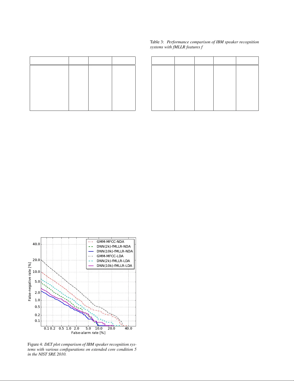
The IBM 2016 Speaker Recognition System Se yed Omid Sadjadi 1 , Sriram Ganapathy 2 ? , J ason W . P elecanos 1 1 IBM Research, Y orkto wn Heights, NY , USA 2 Dept. of Electrical Eng., Indian Institute of Science, Bangalore, India sadjadi@us.ibm.com Abstract In this paper we describe the recent adv ancements made in the IBM i-vector speaker recognition system for con versational speech. In particular , we identify key techniques that con- tribute to significant improv ements in performance of our sys- tem, and quantify their contrib utions. The techniques include: 1) a nearest-neighbor discriminant analysis (ND A) approach that is formulated to alleviate some of the limitations associ- ated with the conv entional linear discriminant analysis (LD A) that assumes Gaussian class-conditional distributions, 2) the ap- plication of speaker- and channel-adapted features, which are deriv ed from an automatic speech recognition (ASR) system, for speaker recognition, and 3) the use of a deep neural net- work (DNN) acoustic model with a large number of output units ( ∼ 10 k senones) to compute the frame-lev el soft align- ments required in the i-vector estimation process. W e ev al- uate these techniques on the NIST 2010 speaker recognition ev aluation (SRE) extended core conditions in volving telephone and microphone trials. Experimental results indicate that: 1) the ND A is more effecti ve (up to 35% relati ve improvement in terms of EER) than the traditional parametric LDA for speaker recognition, 2) when compared to raw acoustic features (e.g., MFCCs), the ASR speaker-adapted features provide gains in speaker recognition performance, and 3) increasing the number of output units in the DNN acoustic model (i.e., increasing the senone set size from 2k to 10k) pro vides consistent improve- ments in performance (for example from 37% to 57% relative EER gains o ver our baseline GMM i-vector system). T o our knowledge, results reported in this paper represent the best per- formances published to date on the NIST SRE 2010 extended core tasks. 1. Introduction There ha ve been significant advancements in the speaker recog- nition field ov er the past few years. The research trend in this field has gradually ev olved from joint factor analy- sis (JF A) based methods, which attempt to model the speaker and channel subspaces separately [1], tow ards the i-vector ap- proach that models both speaker and channel variabilities in a single low-dimensional (e.g., a few hundred) space termed the total variability subspace [2]. State-of-the-art i-v ector based speaker recognition systems employ universal back- ground models (UBM) to generate frame-le vel soft alignments required in the i-vector estimation process. The i-vectors are typically post-processed through a linear discriminant analy- sis (LD A) [3] stage to generate dimensionality reduced and channel-compensated features which can then be efficiently ? This work was done while Sriram Ganapathy was a Research Staf f Member at IBM. modeled and scored with v arious backends such as a probabilis- tic LD A (PLD A) [4, 5]. Until recently , Gaussian mixture models (GMM) trained in an unsupervised fashion (i.e., with no phonetic labels) were commonly used to represent the UBM in speaker recogni- tion. Howe ver , inspired by the success of deep neural net- work (DNN) acoustic models in the automatic speech recogni- tion (ASR) field, [6] proposed the use of DNN senone (context- dependent triphones) posteriors for computing the soft align- ments, which resulted in remarkable reductions in speaker recognition error rates. The performance improvements re- ported in [6] are consistent with the observations made in our earlier ef fort [7] where a supervised GMM-HMM acoustic model (deri ved from an ASR system) was utilized to estimate the hyperparameters of a phonetically inspired UBM (PI-UBM) for speaker recognition. More recently , a supervised GMM- UBM (with full cov ariance matrices) based on DNN posteriors was also successfully ev aluated for telephony speaker recogni- tion [8]. These approaches are motivated by the fact that many of the speaker-dependent characteristics, which are conditioned on some phonetic units/classes, may be more effecti vely mod- eled using a UBM trained with explicit phonetic information. In this paper , we report on the latest advancements made in the IBM i-vector speaker recognition system for con versa- tional speech. Particularly , we first describe key components that contribute to significant improvements in performance of our system. These components include: 1) a nearest-neighbor based discriminant analysis (ND A) approach [9] for channel compensation in i-vector space, which, unlike the commonly used Fisher LD A, is non-parametric and typically of full rank, 2) speaker- and channel-adapted features derived from feature- space maximum likelihood linear regression (fMLLR) trans- forms [10, 11], which are used both to train/e valuate the DNN and to compute the suf ficient Baum-W elch statistics for i-vector extraction, and 3) a DNN acoustic model with a large num- ber of output units ( ∼ 10 k senones) to compute the soft align- ments (i.e., the posteriors). T o quantify the contribution of these components, we e valuate our system in the context of speaker verification experiments using speech material from the NIST 2010 speaker recognition evaluation (SRE) which includes 5 extended core conditions in volving telephone and microphone trials. 2. System Overview In the follo wing subsections, we briefly describe the major com- ponents of our speaker recognition system. Specifically , we first provide an overvie w of GMM- versus DNN-based i-vector ex- traction, which is followed by algorithmic descriptions for the LD A and the NDA for channel compensation in the i-vector space. A schematic block diagram of the system is depicted in i - v ector Extr ac ti on Ac ous ti c Feats . Speech SAD Suf f. Stats Dim. Reduc . T matr i x LDA/NDA PLDA fMLLR Figure 1: Block diagram of the IBM speaker recognition system with fMLLR speaker- and channel-adapted features, DNN posterior based i-vectors, and ND A dimensionality r eduction. Fig. 1. 2.1. I-vector extraction The i-vector representation is based on the total variability modeling concept which assumes that speaker - and channel- dependent v ariabilities reside in the same lo w-dimensional sub- space [2]. The key idea here is that variability within and across sessions can be described via a small set of parameters (a.k.a factors) in a low-dimensional subspace spanned by the columns of a low-rank rectangular matrix, T , entitled the total variability matrix . Mathematically , the adapted mean supervector , M (s), for a giv en set of observations, s , can be modeled as, M ( s ) = m + T x ( s ) +  , (1) where m is the prior mean supervector , x ( s ) ∼ N ( 0 , I ) is a multivariate random variable termed an identity vector “i- vector”, and  ∼ N ( 0 , Σ ) is a residual noise term to account for the variability not captured via T ( Σ is typically copied from the UBM). In other words, for the given observ ation set s , the i-vector represents the coordinates in the total variability subspace. In order to learn the bases for the total variability subspace, one needs to compute the Baum-W elch statistics which are de- fined as, N g ( s ) = X t γ tg ( s ) , (2) F g ( s ) = X t γ tg ( s ) O t ( s ) , (3) where N g ( s ) and F g ( s ) denote the zeroth- and first-order statis- tics for speech session s , respectiv ely , with γ tg ( s ) being the posterior probability of the mixture component g given the ob- servation v ector O t ( s ) at time frame t . The observation vector O t ( s ) can be either the conv en- tional raw acoustic features such as mel-frequency cepstral co- efficients (MFCC) or their speaker- and channel-adapted ver- sions which is computed through a per recording fMLLR trans- form [11, 10] typically obtained with a GMM-HMM system. Note from Fig. 1 that the same fMLLR transformed features can be used to train/ev aluate the DNN as well as compute the sufficient Baum-W elch statistics for i-vector extraction. T raditionally , the frame-lev el soft alignments, γ tg ( s ) , in (2) and (3) are computed with a GMM acoustic model trained in an unsupervised fashion (i.e., with no phonetic labels). How- ev er , in [7], a supervised GMM-HMM acoustic model (deriv ed from a speech recognition system) was utilized to estimate the GMM-UBM hyperparameters for speaker recognition, assum- ing that class-conditional distributions for the various phonetic classes are Gaussian. More recently , inspired by the success of DNN acoustic models in automatic speech recognition (ASR) field, [6] proposed the use of DNN senone (context-dependent triphones) posteriors for computing the soft alignments, γ tg ( s ) , which resulted in remarkable reductions in speaker recognition error rates. Motiv ated by these results, in this paper , we explore the DNN senone posterior based i-vectors for speaker recog- nition, and compare their effecti veness against GMM i-vectors on this task. Furthermore, we also in vestigate the impact of the senone set size on speaker recognition performance. It is worth noting that increasing the number of components in the unsupervised GMM acoustic model (with diagonal cov ariance matrices) for speaker recognition did not seem to result in much performance gains, if at all, in the recent studies [6, 8]. 2.2. Linear discriminant analysis (LD A) As noted before, i-vectors model speaker- and channel- dependent information within the same total variability sub- space. Therefore, in order to select the most relevant fea- ture subset for the speaker recognition task, LD A can be ap- plied to i-vectors to annihilate the directions not informativ e for speaker recognition. In addition, reducing the dimensionality of i-vectors via LD A can improve the computational efficiency of the subsequent backend components in the system. LD A computes an optimum linear projection A : R d 7→ R n , by maximizing the ratio of the inter-class scatter to intra- class variance, where A is a rectangular matrix with n linearly independent columns. Here, the within- and between-class scat- ter matrices are used to formulate a class separability criterion which con verts the matrices into a single statistic. This statistic takes on larger values when the between-class scatter is larger and the within-class variance is smaller . Several such class sep- arability criteria are described in [3], of which the following is the most widely used, ˆ A = arg max A T S w A = I h tr  A T S b A i , (4) where S b and S w denote the between- and within- class scatter matrices, respectively . The optimization problem in (4) has an analytical solution that is a matrix whose columns are the n eigen vectors corresponding to the largest eigenv alues of S − 1 w S b . There are three disadv antages associated with the paramet- ric nature of the scatter matrices S b and S w . First, the under- lying distribution of classes is assumed to be Gaussian with a common covariance matrix for all classes. Therefore, one cannot expect the parametric LD A to generalize well to non- Gaussian and multi-modal (as opposed to unimodal) distribu- tions. It is well known in the speaker recognition community that the actual distribution of i-vectors may not necessarily be Gaussian [12]. This is in particular more problematic when speech recordings are collected in the presence of noise and channel distortions [9, 13]. In addition, for the NIST SRE type of scenarios, speech recordings come from various sources and collects (sometimes out-of-domain), therefore unimodality of the distributions cannot be guaranteed. Second, notice that the rank of S b is C − 1 , which means the parametric LD A can pro- vide at most C − 1 discriminant features. Howe ver , this may not be sufficient in applications such as language recognition where the number of language classes is much smaller than the dimen- sionality of the i-vectors [13]. Nevertheless, this may not pose a challenge for speaker recognition tasks in which the number of training speakers exceeds the dimensionality of the total v ari- ability subspace. Finally , because only the class centroids are taken into account for computing S b , the parametric LD A can- not ef fectiv ely capture the boundary structure between adjacent classes which is essential for classification [3]. T o overcome the abov e noted limitations of LD A, an NDA technique was proposed in [14], that measures both the within- and between-class scatters on a local basis using a nearest neighbor rule. W e have previously e valuated the NDA for both speaker and language recognition tasks on high-frequency (HF) radio channel degraded data [9, 13], where it compared fa vor - ably to the LDA. W e provide a brief description of NDA in the next section. 2.3. Nearest-neighbor discriminant analysis (ND A) In order to alleviate some of the limitations identified for LD A, a nonparametric discriminant analysis techniques was proposed in [14]. In ND A, the expected values that represent the global information about each class are replaced with local sample av erages computed based on the k -NN of individual samples. More specifically , in the ND A approach, the between-class scat- ter matrix is defined as, ˜ S b = C X i =1 C X j =1 j 6 = i N i X l =1 w ij l  x i l − M ij l   x i l − M ij l  T , (5) where x i l denotes the l th sample from class i , and M ij l is the local mean of k -NN samples for x i l from class j which is com- puted as, M ij l = 1 K K X k =1 N N k ( x i l , j ) , (6) where N N k ( x i l , j ) is the k th nearest neighbor of x i l in class j . The weighting function w ij l in (5) is defined as, w ij l = min  d α  x i l , N N K ( x i l , i )  , d α  x i l , N N K ( x i l , j )  d α ( x i l , N N K ( x i l , i )) + d α ( x i l , N N K ( x i l , j )) , (7) where α ∈ R is a constant between zero and infinity , and d ( . ) denotes the distance (e.g., cosine or Euclidean). The weighting function is introduced in (5) to deemphasize the local gradients that are large in magnitude to mitigate their influence on the scatter matrix. The weight parameters approach 0 . 5 for sam- ples near the classification boundary (e.g., see { v 2 , v 3 , v 5 , v 6 } shown in Figure 2), while dropping of f to 0 for samples that are far from the boundary (e.g., see v 4 in Figure 2). The control V 2 V 3 V 1 V 4 V 5 V 6 Figure 2: Symbolic e xample illustrating the parametric versus nonparametric scatter between two classes. v 1 r epr esents the global gr adient of class centr oids. The vectors { v 2 , · · · , v 6 } r epr esent the local gradients. parameter α determines how rapidly such decay in the weights occurs. The nonparametric within-class scatter matrix, ˜ S w , is com- puted in a similar fashion as in (5), except the weighting func- tion is set to 1 and the local gradients are computed within each class. The NDA transform is then formed by calculating the eigen vectors of ˜ S − 1 w ˜ S b . Three important observations can be made from a careful examination of the nonparametric between-class scatter matrix in (5). First, notice that as the number of nearest neighbors, K , approaches N j , the total number of samples in class j , the local mean vector , M ij l , approaches the global mean of class j (i.e., µ j ). In this scenario, if we set the weight parameters to 1 , the ND A transform essentially becomes the LD A projection, which means the LD A is a special case of the more general ND A. Second, because all the samples are taken into account for the calculation of the nonparametric between-class scatter ma- trix (as opposed to only the class centroids), ˜ S b is generally of full rank. This means that unlike the LDA that provides at most C − 1 discriminant features, the ND A generally results in d -dimensional vectors (assuming a d -dimensional input space) for the classification. As we discussed before, this is of great importance for applications such as language recognition where the number of classes is much smaller than the dimensionality of the total subspace (or the input space in general). Finally , compared to LDA, NDA is more effecti ve in pre- serving the comple x structure (i.e., local and boundary struc- ture) within and across different classes. As seen from the example sho wn in Figure 2 (where k is set to 1 for simplic- ity), LDA only uses the global gradient obtained with the cen- troids of the two classes (i.e., v 1 ) to measure the between-class scatter . On the other hand, ND A uses the local gradients (i.e., { v 2 , · · · , v 6 } ) that are emphasized along the boundary through the weighting function, w ij l . Hence, the boundary information becomes embedded into the resulting transformation. 3. Experiments This section provides a description of our experimental setup including speech data, the ASR system configuration, and the speaker recognition (SR) system configuration used in our ev al- uations. T able 1: Description of the 5 core enr ollment/test conditions in the NIST 2010 SRE. Condition Enroll T est Mismatch #T arget T rials #Impostor Trials C1 Interview microphone Intervie w microphone (same type) No 4,034 795,995 C2 Interview microphone Intervie w microphone (different type) Y es 15,084 2,789,534 C3 Interview microphone T elephony Y es 3,989 637,850 C4 Interview microphone Room microphone Y es 3,637 756,775 C5 T elephony T elephony (dif ferent type) Y es 7,169 408,950 3.1. Data W e conduct the core of our speaker recognition experiments using conv ersational telephone and microphone (phone call and intervie w) speech material extracted from datasets released through the linguistic data consortium (LDC) for the NIST 2004-2010 SRE [15, 16], as well as Switchboard Cellular (SWBCELL) P arts I and II and Switchboard2 (SWB2) Phase II and Phase III corpora. These datasets contain speech spo- ken in U.S. English (the non English portion was filtered out) from a lar ge number of male and female speakers with multiple sessions per speaker . The NIST SRE 2010 data is held out for ev aluations, while the remaining data are used to train the sys- tem hyper -parameters (i.e., the i-v ector extractor , LDA/ND A, and PLD A). There are a total of 5 e xtended core tasks in the NIST SRE 2010 that in volv e telephone and microphone trials from both male and female speakers [17]. A more detailed de- scription of the 5 tasks is presented in T able 1. 3.2. DNN system configuration The architecture of the DNN acoustic model used to generate the soft alignments for i-vector extraction is sho wn in Fig. 3. The model, which has 7 fully connected hidden layers with 2048 units per layer except for the bottleneck layer that has 512 units, is discriminativ ely trained using the standard error back-propagation and cross-entropy objective function to esti- mate posterior probabilities of 10,000 senones (HMM triphone states). The training is accomplished using the IBM Attila toolkit [18] on 600 hours of conv ersational telephone speech (CTS) data from the Fisher corpus [19] with a 9-frame con- text of 40-dimensional speaker -adapted feature vectors obtained 1 0 ,0 0 0 512 2 ,0 4 8 2 ,0 4 8 2, 04 8 2 ,0 4 8 2 ,0 4 8 9 x 4 0 2 ,0 4 8 Figure 3: Arc hitectur e of the DNN acoustic model with 7 hidden layers used in our speaker r ecognition experiments. through per recording fMLLR transforms [10, 11]. The fM- LLR transforms are generated for each recording with decoding alignments obtained from a GMM-HMM acoustic model. The GMM models are trained with 40-dimensional features which are deriv ed from 13-dimensional MFCCs as follow; the base cepstral features from 9 consecutive frames are first spliced af- ter cepstral mean-variance and vocal tract length normalizations (VTLN). An LD A transform is then applied to reduce the fi- nal feature vector dimensionality to 40. The range of the LDA transformation is diagonalized by means of a global semi-tied cov ariance transform (see [20, 21] for more details). In addition to running experiments with all the 10k senones, we also ex- plore smaller senone set sizes of 2k and 4k which are obtained by merging the 10k HMM states using a phonetic decision tree with maximum-likelihood (ML) criterion [22]. 3.3. SR system configuration For speech parameterization (other than the fMLLR based fea- tures), we extract 13-dimensional MFCCs (including c 0 ) from 25 ms frames every 10 ms using a 24-channel mel filterbank spanning the frequency range 200-3500 Hz. The first and sec- ond temporal cepstral deri v ativ es are also computed ov er a 5- frame window and appended to the static features to capture the dynamic pattern of speech o ver time. This results in 39- dimensional feature vectors. For non-speech frame dropping, we employ an unsupervised speech activity detector (SAD) based on voicing ener gy features [23]. After dropping the non- speech frames, global (recording level) cepstral mean and vari- ance normalization (CMVN) is applied to suppress the short term linear channel effects. In this paper , a 500-dimensional total v ariability subspace is learned and used to extract i-vectors from the recordings. T o learn the i-vector extractor , out of a total of 60,178 recordings av ailable from 1884 male and 2601 female speakers, we se- lect 48,325 recordings from the NIST SRE 2004-2008, SWB- CELL, and SWB2 corpora. The zeroth and first order Baum- W elch statistics are computed for each recording using soft alignments obtained from either a gender-independent 2048- component GMM-UBM with diagonal covariance matrices, or the DNN acoustic model with 2k, 4k, and 10k senones. The GMM-UBM is trained using 21,207 recordings selected from the NIST SRE 2004-2006, SWBCELL, and SWB2 corpora. After extracting 500-dimensional i-vectors, we either use LD A or NDA for inter -session variability compensation by re- ducing the dimensionality to 250. In order to train the ND A, we employ a one-versus-rest strategy to compute the inter-speaker scatter matrix in (5). This provides flexibility on the number of nearest neighbors used for computing the local means. A co- sine similarity metric (as opposed to Euclidean) is used to find T able 2: P erformance comparison of IBM speaker r ecognition systems with various configur ations on e xtended cor e condition 5 in the NIST SRE 2010. A DNN with 10k senones is used. System EER [%] minDCF08 minDCF10 GMM-MFCC-LD A 2.40 0.120 0.439 GMM-MFCC-ND A 1.55 0.076 0.286 DNN-MFCC-LD A 1.02 0.045 0.168 DNN-MFCC-ND A 0.76 0.036 0.147 DNN-fMLLR-LD A 0.82 0.032 0.120 DNN-fMLLR-ND A 0.67 0.028 0.092 the k -nearest neighbors for each sample, and the exponent α in (7) is set to 1 . The dimensionality reduced i-vectors are then centered (the mean is remov ed), whitened, and unit-length nor- malized. For scoring, a Gaussian PLDA model with a full co- variance residual noise term [4, 5] is learned using the i-v ectors extracted from all 60,178 speech se gments (1884 male and 2601 female speakers) as noted previously . The Eigen voice subspace in the PLD A model is assumed full-rank. 4. Results and Discussion In this section, we summarize our results obtained with the ex- perimental setup presented in Section 3. In the first experiment, we e valuated the effecti veness of the NDA versus the LD A for inter-session v ariability compensation and dimensionality re- duction in the i-vector space. The outcome of this experiment is presented in T able 2 for the NIST SRE 2010 extended “tel-tel” trials (condition 5), in terms of the equal error rate (EER), mini- mum detection cost function with the NIST SRE 2008 [24] and 2010 [17] definitions (minDCF08 and minDCF10). It can be seen from the table that the systems with the NDA consistently 0.1 0.2 0.5 1.0 2.0 5.0 10.0 20.0 40.0 False-alarm rate [%] 0.1 0.2 0.5 1.0 2.0 5.0 10.0 20.0 40.0 False-negative rate [%] GMM-MFCC-NDA DNN(2k)-fMLLR-NDA DNN(10k)-fMLLR-NDA GMM-MFCC-LDA DNN(2k)-fMLLR-LDA DNN(10k)-fMLLR-LDA Figure 4: DET plot comparison of IBM speaker r ecognition sys- tems with various configurations on extended core condition 5 in the NIST SRE 2010. T able 3: P erformance comparison of IBM speaker r ecognition systems with fMLLR featur es for 2k, 4k, and 10k DNN senones on extended cor e condition 5 in the NIST SRE 2010. System #Senones EER [%] minDCF08 minDCF10 DNN-LD A 2k 1.19 0.054 0.212 DNN-ND A 2k 0.95 0.043 0.166 DNN-LD A 4k 0.98 0.041 0.169 DNN-ND A 4k 0.86 0.033 0.116 DNN-LD A 10k 0.82 0.032 0.120 DNN-ND A 10k 0.67 0.028 0.092 provide better speaker recognition performance across all three metrics. For the GMM based system, a relativ e improvement of 35% in EER is achiev ed with the NDA ov er the LD A, while for the DNN based systems with MFCCs and fMLLR features relativ e impro vements of 26% and 18% are obtained, respec- tiv ely . As we discussed before, this is due to the nonparametric representations for the scatter matrices in NDA that makes no assumptions reg arding the underlying class-conditional distri- butions. In addition, ND A is more ef fectiv e in capturing the local structure (as opposed to global bulk structure) and bound- ary information within and across dif ferent speakers. Another important observ ation that can be made from T able 2 is that, irrespectiv e of the dimensionality reduction algorithm used, the systems with fMLLR features outperform the MFCC based sys- tems. This is attributed to the ability of the fMLLR transforms in reducing the speaker and channel variabilities in the acoustic feature space. In the next set of experiments, we in vestigated the impact of the number of senones on speaker recognition performance. T a- ble 3 shows speaker recognition results on the NIST SRE 2010 “tel-tel” condition which are obtained with i-vectors computed using 2k, 4k, and 10k DNN senones and fMLLR features. T wo important observations can be made from this table. First, the larger the number of senones, the better the performance. This is due to the discriminativ e nature of the DNN where increas- ing the granularity in the output layer improv es the model abil- ity in distinguishing among the v arious phonetic ev ents. It is worth noting that increasing the number of components in the unsupervised GMM acoustic model (with diagonal cov ariance matrices) for speaker recognition did not result in much per- formance improv ements in the recent studies [6, 8]. Second, irrespectiv e of the number of senones used to calculate the suf- ficient statistics, the NDA based systems consistently perform better than the LD A based systems. W e note that, in our exper - iments, increasing the number of senones be yond 10k did not yield much gains in performance. Fig. 4 sho ws the detection error trade-off (DET) curves for the ND A and LD A based systems on the e xtended core con- dition 5 in the NIST SRE 2010. Consistent with our previous observations, it is seen that the ND A based systems achiev e the best performance across a wide range of operating points on the DET curves. The performance gap between the ND A and LD A based systems is, howe ver , reduced when DNN senone posteri- ors are used to compute the i-vectors, and increasing the senone set size from 2k to 10k further narrows this g ap. For completeness, we also ev aluated the performance of our speaker recognition system on extended microphone and T able 4: P erformance comparison of IBM speaker r ecognition systems with various configurations on extended micr ophone and tele- phone conditions (C1–C4) in the NIST SRE 2010. A DNN model with 10k senones is used. System EER [%] minDCF08 minDCF10 C1 C2 C3 C4 C1 C2 C3 C4 C1 C2 C3 C4 GMM-MFCC-ND A 1.39 1.89 1.80 1.46 0.053 0.084 0.081 0.061 0.215 0.313 0.315 0.251 DNN-MFCC-ND A 0.84 1.41 0.83 0.63 0.027 0.046 0.036 0.022 0.104 0.157 0.127 0.103 DNN-fMLLR-ND A 1.02 1.44 0.90 0.77 0.033 0.049 0.034 0.025 0.112 0.158 0.119 0.096 telephone conditions (C1–C4) in the NIST SRE 2010. The re- sults are provided in T able 4 for both the GMM and DNN based systems. It is clear that the DNN based systems, with either MFCCs or fMLLR features, perform significantly better than the GMM based system. Additionally , the DNN based system trained with raw MFCCs tend to perform better than the fM- LLR based system, at least in terms of EER. W e speculate that this is because the fMLLR transforms, which are obtained us- ing GMM-HMMs trained only on telephon y data, are unable to effecti vely reduce the v ariability due to channel mismatch on microphone recordings. 5. Conclusions In this paper, we presented the recent improv ements made in our state-of-the-art i-vector speaker recognition system. W e in- vestigated the impact of several key components of the system on performance using extended core tasks in the NIST 2010 SRE that in volved both microphone and telephone trials. Some important observ ations made from our experiments were as fol- lows: 1) the ND A was found to be consistently more ef fectiv e than the LDA for inter-session variability compensation in i- vector based speaker recognition, 2) the fMLLR based features provided better representation than raw MFCCs for matched data conditions (i.e., telephony trials), and 3) the DNN based UBM with large number of components (i.e., 10k senones) re- sulted in remarkable improv ements in the performance of our system. T o the best of our knowledge, the results presented in this paper represent the best performances reported to date on the extended core tasks in the NIST 2010 SRE. 6. References [1] P . Kenny , G. Boulianne, P . Ouellet, and P . Dumouchel, “Joint factor analysis versus eigenchannels in speaker recognition, ” IEEE T rans. Audio Speech Lang. Process. , vol. 15, no. 4, pp. 1435–1447, 2007. [2] N. Dehak, P . Kenny , R. Dehak, P . Dumouchel, and P . Ouellet, “Front-end factor analysis for speaker verifica- tion, ” IEEE T rans. Audio Speech Lang. Pr ocess. , vol. 19, no. 4, pp. 788–798, 2011. [3] K. Fukunaga, Intr oduction to Statistical P attern Recogni- tion , 2nd ed. New Y ork: Academic press, 1990. [4] S. J. Prince and J. H. Elder , “Probabilistic linear discrimi- nant analysis for inferences about identity , ” in Pr oc. IEEE ICCV , Rio De Janeiro, October 2007, pp. 1–8. [5] D. Garcia-Romero and C. Y . Espy-W ilson, “ Analysis of i-vector length normalization in speaker recognition sys- tems. ” in Pr oc. INTERSPEECH , Florence, Italy , August 2011, pp. 249–252. [6] Y . Lei, N. Scheffer , L. Ferrer , and M. McLaren, “ A novel scheme for speaker recognition using a phonetically- aware deep neural network, ” in Proc. IEEE ICASSP , Flo- rence, Italy , May 2014, pp. 1695–1699. [7] M. K. Omar and J. Pelecanos, “T raining univ ersal back- ground models for speaker recognition, ” in Pr oc. The Speaker and Language Recognition W orkshop (Odysse y 2010) , Brno, Czech, June 2010, pp. 52–57. [8] D. Snyder , D. Garcia-Romero, and D. Pove y , “Time delay deep neural network-based uni versal background models for speak er recognition, ” in Pr oc. IEEE ASR U , Scottsdale, AZ, December 2015, pp. 92–97. [9] S. O. Sadjadi, J. W . Pelecanos, and W . Zhu, “Nearest neighbor discriminant analysis for robust speaker recog- nition, ” in Pr oc. INTERSPEECH , Singapore, Singapore, September 2014, pp. 1860–1864. [10] V . Digalakis, D. Rtische v , and L. Neumeyer , “Speaker adaptation using constrained estimation of Gaussian mix- tures, ” IEEE T rans. Speech Audio Pr ocess. , vol. 3, no. 5, pp. 357–366, September 1995. [11] M. J. F . Gales, “Maximum likelihood linear transfor- mations for HMM-based speech recognition, ” Comput. Speech Lang . , vol. 12, no. 2, pp. 75–98, 1998. [12] P . Kenn y , “Bayesian speaker verification with hea vy tailed priors, ” in Proc. The Speaker and Language Recognition W orkshop (Odysse y 2010) , Brno, Czech, June 2010. [13] S. O. Sadjadi, S. Ganapathy , and J. W . Pelecanos, “Nearest neighbor discriminant analysis for language recognition, ” in Pr oc. IEEE ICASSP , Brisbane, Australia, April 2015, pp. 4205–4209. [14] K. Fukunaga and J. Mantock, “Nonparametric discrimi- nant analysis, ” IEEE T rans. P attern Anal. Mach. Intell. , vol. 5, no. 6, pp. 671–678, 1983. [15] C. Cieri, L. Corson, D. Graf f, and K. W alker , “Re- sources for new research directions in speaker recognition: The Mixer 3, 4 and 5 corpora, ” in Pr oc.INTERSPEECH , Antwerp, Belgium, August 2007, pp. 950–953. [16] L. Brandschain, D. Graf f, C. Cieri, K. W alker , C. Caruso, and A. Neely , “Mixer 6, ” in Pr oc. LREC , V alletta, Malta, May 2010. [17] NIST , “The NIST Y ear 2010 Speaker Recognition Evalu- ation Plan, ” http://www .nist.gov/itl/iad/mig/upload/NIST SRE10 e valplan- r6.pdf, 2010. [18] H. Soltau, G. Saon, and B. Kingsb ury , “The IBM Attila speech recognition toolkit, ” in Pr oc. IEEE SLT , Berkeley , CA, December 2010, pp. 97–102. [19] C. Cieri, D. Miller , and K. W alker , “The Fisher corpus: A resource for the next generations of speech-to-text, ” in Pr oc. LREC , Lisbon, Portugal, May 2004. [20] S. Ganapathy , S. Thomas, D. Dimitriadis, and S. Ren- nie, “In vestigating f actor analysis features for deep neural networks in noisy speech recognition, ” in Pr oc. INTER- SPEECH , Dresden, Germany , September 2015, pp. 1898– 1902. [21] G. Saon, H. K. Kuo, S. Rennie, and M. Picheny , “The IBM 2015 English con versational telephone speech recog- nition system, ” in Pr oc. INTERSPEECH , Dresden, Ger- many , September 2015, pp. 3140–3144. [22] S. J. Y oung, J. J. Odell, and P . C. W oodland, “T ree-based state tying for high accuracy acoustic modelling, ” in Pr oc. W orkshop Human Lang. T ech. , March 1994, pp. 307–312. [23] S. O. Sadjadi and J. H. L. Hansen, “Unsupervised speech activity detection using voicing measures and perceptual spectral flux, ” IEEE Signal Pr ocess. Lett. , vol. 20, no. 3, pp. 197–200, 2013. [24] NIST , “The NIST Y ear 2008 Speaker Recognition Ev alua- tion Plan, ” http://www .itl.nist.gov/iad/mig/tests/sre/2008/ sre08 ev alplan release4.pdf, 2008.