A note on basis dimension selection in generalized additive modelling

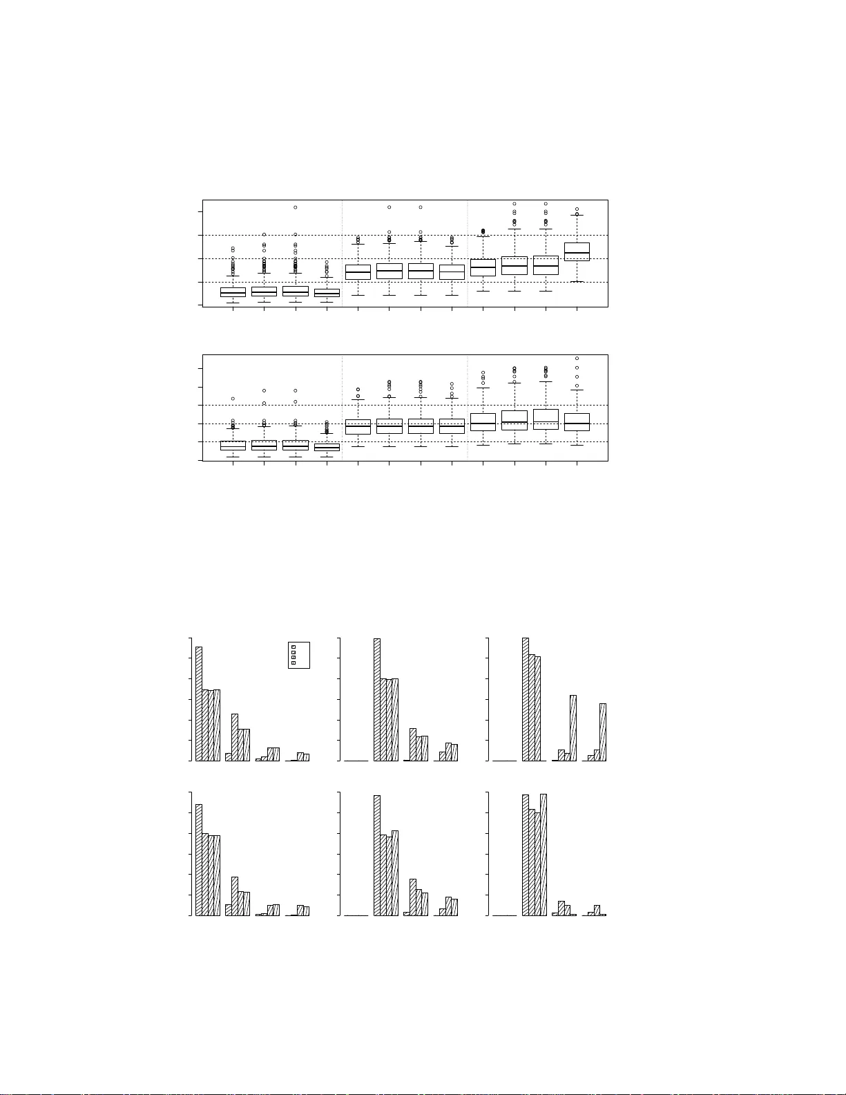
A note on basis dimensi on selection in genera lized additi ve modelling Natalya Pya and Simon N W ood ∗ Nazarbaye v University and Uni versity of Br istol February 23, 2016 Abstract T wo new approa ches for checking th e dimension o f th e basis f unctions wh en using pe nalized regression smoothers a re p resented. The first approa ch is a test f or adeq uacy of the basis d imension based on an estimate of the residual v ar iance calculated by differencing residuals that are neighb ours accordin g to the smoo th covariates. The seco nd app roach is based o n e stimated d egrees of freedo m for a smooth of the mo del residua ls with respect to the model covariates. In co mparison with b asis dimension selection alg orithms based on smoothness selection cr iterion (GCV , AIC, REML) the above procedures are compu tationally efficient enough for routine use as part of model checking. 1 Introd uction Penalized re gression smoothing splines ha ve been use d exten si vely for repres entati on of smooth mod el terms in generaliz ed ad ditiv e modelli ng [O’Sulliv an, 1986 , Eilers and Marx, 1996, W ood, 2006]. In com- pariso n w ith fu ll rank smoo thing splines [W ahba, 1990, Gu, 2002 ], with a free para m eter for each data point, penalized regressi on sp lines ar e computationa lly at tracti ve as the basis dimension, k , is set t o much less than the number of data p oints. Provide d tha t k is la r ge enough to a void o versmooth ing/un derfitting, its e xact v alue is rather unimport ant, since ov erfitting and the ef fectiv e degrees of freedo m of the s mooth are then con trolled by the weight g i ven to the smoothi ng pe nalty during estimatio n, which is determin ed by the smoo thing pa rameter , λ , rat her than k . Ho wev er it is necessary to check that k really is large enoug h, and here useful readily applied ch ecking metho ds are lacking . The choice of k has not bee n w idely discussed in the liter ature. Ruppe rt [20 02 ] pro posed two algo- rithms bas ed on minimiz ing G CV o ver a set of spec ified basis dimen sions. H e demo nstrate d empirica lly that there is a minimal threshold for th e number of knots ne eded for a good fit, larger n umbers of knots ha ve only slight influence on the fit. Theoretic al justification s are pr esente d in Li and Ruppert [2008] who also sho w that the threshol d depends on the degre e of the splin e order . Kau ermann an d Opsomer [2011] intr oduce d a lik elihood based criterion for selec ting k in the cas e of the mixed-mod el speci fica- tion of the penalized spl ine [Ruppert et al., 2003, W and an d Ormerod, 200 8]. In this specificat ion the smoothin g parameter λ , is represented as the rat io of the residual varian ce and the va riance of the spline coef ficients which all o w s estimating λ simultaneo usly w ith the coef ficients by li keli hood max imizatio n. This is equi vale nt to t he restricted maximum like lihoo d criteri on, REML [W ood, 20 06]. k is treated as an ∗ simon.wood@ba th.edu 1 additi onal discrete parame ter of the log likelih ood in Kauerman n and Opsomer [2011]. T wo nested op- timizatio ns are proposed for parameters es timation : for ea ch va lue for k log lik elihood is re-maximized with respe ct to m odel paramete rs. Searchin g for the ‘optimal’ k is clearly a comp utatio nally expe nsi ve op tion, and ar guably of limited practic al uti lity gi ven th e empirica l and the oretic al evide nce that all th at really matters is that k is not to o small. This note therefo re propose s two computatio nally ef ficient approa ches for checking the adequa cy of the ba sis dimension from a fitted model, and comp ares their practica l efficac y to a fuller se arch for an optimal k , in a small simulatio n stu dy . 2 Methods f or checking the basis dimension W e consider a genera lized ad diti ve model g ( µ i ) = A θ + p X j =1 f j ( x j i ) , Y i ∼ EF( µ i , φ ) , i = 1 , . . . , n, (1) where Y i are independe nt univ ariate res ponse v ariables from an expone ntial f amily dis trib ution with mean µ i and sca le parameter φ , g is a kn own smooth monotoni c link function, A is a model matrix, θ is a vec tor of unkno wn parameters, f j is an unkno wn smooth function of predictor var iable x j that may be vec tor v alued. For representing the smooth function s f j ( x j ) v arious penalized regress ion smoother s are a vail able, such as cubi c re gression spline s and P-splines for smooths of a single co vari ate, or thin pla te re gression spline s and tensor pro duct smooth s for repr esenti ng smo oths of s e veral cov ariates. T he ide a is to specify a basis for each function and choose an appr opriate set of basis functions, B j t , so that the j th smooth functi on ca n be represe nted as f j ( x j ) = k j X t =1 B j t ( x j ) β j t , where β j t are c oef ficients to be estimated, and k j is a numb er of basis functio ns. After selecting smoot h- ing penalties for each smooth function, the penal ized log likelihoo d functio n is maximized to get esti- mates of β j t gi ven smoothing parameter s. The smoothing paramet ers, λ j , contr olling the strength of penali zation can be estimated b y optimizi ng criteria such as G CV , AIC, or REML. Although the smoot hness of each smooth term in (1) is controlle d by the smooth ing parameter , λ j , the basis di mension k j used for s mooth rep resent ation needs to b e suf ficiently lar ge to a voi d ov ersmoothing . T o ensure that k j is adequ ate the follo wing ap proach es will be consider ed 1. A hypot hesis testing approac h based on comparison of the resid ual v ariance estimate from the whole model fit, with th e resi dual va riance estimat ed by dif ferencin g residuals that are ‘n eigh- bours’ accord ing to th e cov ariates of the smooth term under considera tion. 2. A proced ure based on re-smoothing the model resid uals with respec t to the cov ariates of the smooth of inter est, using a higher basi s di mension , in order to search fo r missed pattern in the residu als. 3. Optimizing the GCV or REML criterio n with respect to the basis dimensions, as w ell as the smoothin g parameters. The first two proce dures do not seem to ha ve appeared in the literatu re, while t he third is essentially what is propose d in Ruppert [2002 ] and Kauer mann and Opsomer [2011]. Option 1 is simple and efficient enoug h for routine automatic us e. 2 2.1 Hypothesis testing appr o ach T o test whet her k j is suf ficiently lar ge for rep resent ing f j ( x j ) the fo llo wing test is pro posed . Let r i denote dev iance residuals for the m odel that inc ludes f j ( x j ) , in the Gaussian case simply r i = y i − ˆ µ i . First conside r a smooth of a univ ariate x j . Let ˜ r denote the v ector o f residuals r i , ord ered accord ing to the v alues of the obser ved cov ariates, x j i . D efine ∆ i = ˜ r i +1 − ˜ r i for i = 1 , . . . , n − 1 . Then φ ∆ = 1 2 n − 2 P n − 1 i =1 ∆ 2 i is an estimate of the scale pa rameter , a nd if ˆ φ is the cor respon ding estimate from the model fit, we can define a statisti c κ = φ ∆ / ˆ φ which should be cl ose to one if the basis dimension is adequate, bu t sho uld be less than one if k j is too small so that there is residu al pattern left in the residua ls. In the c ase o f multi varia te x j , th en th e M n earest n eighb ours of e ach o bserva tion can be fo und based on th e pro ximity of x j vec tors. This has relati vely modest total cost O ( nM log( n )) , see Press et al. (2007 ). Let m ij be the index of the j th neare st neighbo ur of obse rv ation i (exclu ding self). Then we define ∆ ij = r i − r m ij for i = 1 , . . . n , j = 1 , . . . , M , and φ ∆ = 1 2 M n P M j =1 P n i =1 ∆ 2 ij . The ex pressi on for κ is as before. The dis trib ution of κ under the nu ll hypothesis that k j is ad equate (so that there is no pattern in the residu als orde red wit h respec t to the c ov ariate), can be s imulated by repeatedl y rando mly re-shu ffling th e origin al v ector of residu als, and re- computi ng κ for each replicate. A p-v alue can then be obtained. If it is too small, we shou ld co nside r increasing k j . 2.2 Residual re -smoothing A secon d simple method for checkin g k j is as follo ws. 1. Fit the model with your choice of k j and ext ract the de viance res iduals , r i , i = 1 , . . . , n . 2. Create a smoot h, f ∗ j ( x j ) , equi v alent to f j ( x j ) , b ut with basis di mension 2 k j , then estimate the model r i = f ∗ j ( x j i ) + e i , 3. If the estimate o f f ∗ j indica tes that ther e is pattern in the resi duals (e.g. if the effec tive degrees of freedo m of ˆ f ∗ is more than the minimum possi ble for such a smoot h) then k j may not be lar ge enoug h, and an in crease of k j should be consid ered. It is al so wort h consi dering changes in the smo othing select ion criterion after fitting with increased k j . If the valu e of the criterion is increased or the decre ase is not m ore than 2% of the pre vious valu e, then it is sugges ted to stop doublin g k j since it is not exp ected to impro ve the criterion [Ruppert, 2002]. 2.3 GCV/REML based appr oach The fi nal approach is the simplest, b ut also the lea st computatio nally ef ficient. The idea is simply to search o ver a spec ifi ed set k j v alues for the optimize r of the criter ion used for smoothi ng parameter esti- mation. T he full model has to be re-fitted for each set of trial values of k j , so this is quite costly compu- tation ally . Suc h alg orithms were p roposed first by Rupp ert an d Carro ll [2000] an d Rupp ert [2002] f or P- spline s with the basi s dimension selec tion by minimizing the GC V criterion, w hile K auermann and Opsomer [2011] sugge sts a s imilar like lihood based method . 3 0.0 0.2 0.4 0.6 0.8 1.0 −0.5 0.0 0.5 1.0 1.5 (a) x y 0.0 0.2 0.4 0.6 0.8 1.0 −0.5 0.5 1.5 2.5 (b) x y 0.0 0.2 0.4 0.6 0.8 1.0 −1.5 −0.5 0.5 (c) x y Figure 1: Shapes of the uni v ariate test func tions used for simulation study . 3 Illustrative simulated examples The approaches were compar ed on five simulated ex amples of Gaussian data: three uni vari ate single smooth models follo wing Rupper t [2002], a biv ariate single smooth model and an add iti ve model with two smoo th terms. y i = f t ( x i ) + e i , t = 1 , 2 , 3 , y i = f ( x 1 i , x 2 i ) + e i , y i = f 1 ( x 1 i ) + f 2 ( x 2 i ) + e i , e i ∼ N (0 , σ 2 ) . For all examples data were simulated ind epend ently from y i ∼ N ( µ i , 0 . 2 2 ) . For uni varia te cases x i were equal ly sp aced on [0 , 1] . Three test funct ions f t ( x i ) with shap es shown in Fig. 1 were applied. For sample sizes n = 100 and 2 00 , 30 0 replicate s were simulate d. Each single smooth regress ion m odel was fi t usin g the R pack age mgc v [W ood, 2006]. T hin plate regressio n splines with the second order deri vati ve in p enalty were used fo r representatio n of all smooths [W ood, 200 3]. The basis dimension was selecte d by the approaches presented in section 2. F or methods 1 and 2 the basis dimen sion for a term was doubled if the check suggested th at the current dimension wa s inadeq uate. T wo v ariants of method 3 were tried , one using GCV and the ot her REM L. T he tested v alues of k were 10, 20, 40, 80. The performanc e of the all methods w as ev aluate d by the mean sum of squared dif ferences be tween the fitted, ˆ f ( x ) , and true val ues of f t ( x ) , MSE = n − 1 n X i =1 n ˆ f ( x i ) − f t ( x i ) o 2 . The results are summariz ed in Fig. 2. Fig. 3 sho ws bar plots of k sele cted by the four algorithms. The simulatio n results sh o w that the perfor mance of al l fou r alg orithms is q uite similar e xcepting REML when fi tting the s ine f unctio n with n = 100 . In t hat c ase REML tended to select a lar ger basis dimen sion than other methods which resulted in lar ger MSE . The basis dimensions required for fitting the f 1 are around 10 – 20 which is typical for man y monoton e functions used in practic e. It is clear th at k = 10 is too small for the ‘bump’ fu nction f 2 and sine wa ves with six c ycles f 3 . A ll alg orithms selected at lea st 4 pv sm gcv reml pv sm gcv reml pv sm gcv reml 0.000 0.005 0.010 0.015 0.020 MSE f 1 f 2 f 3 pv sm gcv reml pv sm gcv reml pv sm gcv reml 0.000 0.004 0.008 MSE f 1 f 2 f 3 Figure 2: MS E comparison between h ypothe sis testing approach ( pv ), resi duals smoothin g ( sm ), GCV search ( gcv ), an d REML searc h ( reml ) method s for th ree sing le uni variat e smooth term model s. T he upper panel sho ws the re sults for n = 100 , the lower for n = 200 . 10 20 40 80 pv sm gcv reml frequency 0 50 100 150 200 250 300 f 1 10 20 40 80 0 50 100 150 200 250 300 f 2 10 20 40 80 0 50 100 150 200 250 300 f 3 10 20 40 80 frequency 0 50 100 150 200 250 300 f 1 10 20 40 80 0 50 100 150 200 250 300 f 2 10 20 40 80 0 50 100 150 200 250 300 f 3 Figure 3: Bar plots of k selected by the hyp othesis testing app roach ( pv ), residual s smoothing ( sm ), GCV search ( gcv ), and REML search ( re ml ) methods for three single uni v ariate smooth term models. Three upper pane ls show the results for n = 100 , the lower p anels for n = 200 . 5 x1 x2 f pv sm gcv reml pv sm gcv reml 0.002 0.004 0.006 0.008 MSE n = 400 n = 900 15 30 60 120 pv sm gcv reml frequency 0 50 100 150 200 n = 400 15 30 60 120 frequency 0 50 100 150 200 n = 900 Figure 4: Plots for biv ariate example. Upper left: perspect i ve plot of the biv ariate test functi on; upper right: MSE comparison between four approa ches; lower left: bar plots o f k selected fo r n = 400 ; lower right: bar plots of k selected for n = 900 . 20 basis functions to gi ve satisfac tory fits for those much ‘wigg lier’ functions. It can be noticed that the hypot hesis testing approach stops earlier and chooses smaller b asis dimensio ns compared to the other methods . The shape of the bi va riate te st fu nction use d in the nex t e xample is s ho wn in Fig. 4. 20 a nd 30 v alues of each o f the two co variat es, x 1 i and x 2 i , were equi distan t in [ − 1 , 3] and [0 , 1] , g i ving samples of sizes n = 400 and 900 . 200 repli cate data sets were simulated for each sample size. T he trial value s of the basis dimension were 15, 30, 60, and 120. While sett ing k = 15 is t oo low for all the approach es, k = 30 appear ed to be en ough with only GCV choo sing occasion ally larger k for n = 40 0 and more often for n = 900 (see Fig. 4). The last e xample is an additi ve model with two smo oth terms, y i = f 1 ( x 1 i ) + f 2 ( x 2 i ) + e i , where f 1 is the first functi on used in th e uni variate case and f 2 is a sine funct ion with a single cycle . x 1 i and x 2 i were i.i.d. U (0 , 1) . Sample size s n = 200 and 400 were considered. The simulation result s of this study base d on 200 repl icates are sho wn in Fig. 5. The beha viour of all algorithms is similar to th at of the univ ariate examp le. Ho w e ver , the main benefit of th e hypothes is testing and re-smoothing residu als approa ches is in their computa tional efficien cy . The G CV/REML algorithms require the w hole model to be re-fitted at ev ery combi nation of ( k 1 , k 2 ) values ov er the specified grid. But the hy pothes is testing approa ch needs only calculating the estimate of the residual var iance and its p-valu e. And the secon d approa ch requires re-s moothin g of a singl e term rather th an the whole model. R e-fitting the whole model with an in crease d value of the suspect ed k j occurs only in case of a lo w p-v alue or high edf for the particu lar smooth te rm. The computation al adv antage gro ws with the number of smooth terms in the GAM. 6 pv sm gcv reml pv sm gcv reml 0.002 0.004 0.006 0.008 MSE n = 200 n = 400 10 20 40 80 pv sm gcv reml frequency 0 50 100 150 200 k 1 , n = 200 10 20 40 80 frequency 0 50 100 150 200 k 2 , n = 200 10 20 40 80 frequency 0 50 100 150 200 k 1 , n = 400 10 20 40 80 frequency 0 50 100 150 200 k 2 , n = 400 Figure 5: Plots for the ad ditiv e model. Upper left: boxplots of th e MSE of four ap proach es for n = 200 and 400 ; upper m iddle and right : bar plots of k 1 and k 2 selecte d for two smooth terms, f 1 and f 2 , for n = 200 ; lower p anels: bar plot s of k i for two smoot hs for n = 400 . 4 Conclusions In pract ice the simple and ef ficient basis dimension check propos ed in Section 2.1 appear s to perform as well as more expen si ve approa ches requi ring m ultipl e m odel fits. Giv en its computa tional ef ficiency it seems sensible to inco rporate this check as a standard part of model check ing for pena lized re gressi on spline based generalize d additi ve models. Of course as with any model checking, the methods hav e to be us ed with care. Mean v ariance relations hip problems and residu al au tocorr elation problems unrelated to k j can ob viously cause any of the methods consider ed he re to suggest increasin g k j , when the real proble m li es else where. This work was s upported by EPSRC gra nts EP/K005251/1 and EP/1000917/1 Refer ences P .H. Eilers and B.D. Marx. Flexib le smoothing w ith B-splines and penalties. S tatistical Scie nce , 11: 89–12 1, 1996. C. Gu. Smooth ing Spline ANO V A Models . Ne w Y ork: Springer , 2002. G. Kauermann and J.D. Opso mer . Data-dri ven select ion of th e spline dimen sion in pen alized spline reg ression . Biometrika , 98(1):22 5–230, 2011. Y . Li and D. Ruppert. On the asympto tics of penal ized sp lines. Biometrika , 95(2) :415–436, 2008. F . O’Sulli van. A stati stical perspecti ve o n ill-po sed in verse proble ms. Stat istical Science , 1:50 2–518, 1986. 7 D. Ruppert. Selecting the number of kno ts for penali zed spli nes. Jour nal of Compu tation al and Grap h- ical Statis tics , 1 1(4):7 35–75 7, 2002. D. Ruppert and R.J. C arroll. Spatially-ad aptiv e penal ties for spli ne fittin g. Au str alian and N ew Zeal and J ournal of St atistic s , 42:205 –223, 20 00. D. Ruppert, M.P . W an d, a nd R.J. Carroll. Semiparamet ric Re gr ession . New Y ork: Cambrid ge Uni versi ty Press, 2003 . G. W ahba. Spline models for observ ational data . Philadel phia: SIAM, 1990 . M.P . W and and J.T . Ormerod. On semipa rametric regressio n with o’ su lli van penalized splines. Austr alian and New Zeal and Jou rnal of Statist ics , 50 (2), 2008 . S.N. W ood. Thin plate re gression splines. J ournal of the R oyal Stat istica l So ciety: Series B , 65(1): 95–11 4, 2003. S.N. W ood. Gener alized Additive Models. An Intr oduc tion with R . Chapman & Hal l, 20 06. 8