Burstiness Scale: a highly parsimonious model for characterizing random series of events

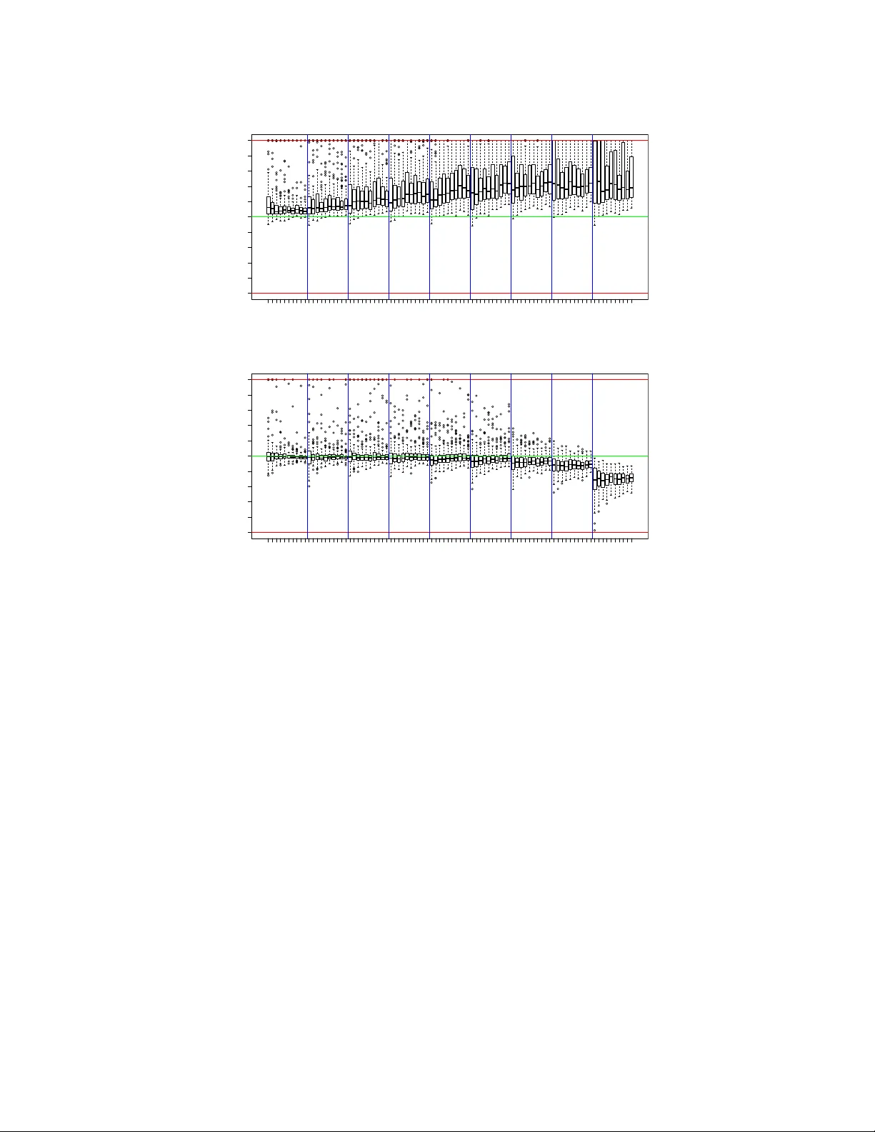
A Burstiness Sc ale: a highly par simonious model f or charac terizing random series of ev ents Rodrigo A S Alve s , CEFE T -MG Renato Assunção , UFMG P edro O.S . V az de Melo , UFMG The problem to accu rately and parsimoniously charac terize random series of ev ents (RSEs) present in the W eb, suc h as e-mail con versat ions or T witte r hashtags, is not t ri vial. Reports found in t he lite rature rev eal two appa rent conﬂicti ng visions of ho w RSEs should be modeled. From one side, t he Poissonian processes, of which consecuti ve eve nts follow each other at a relati vely regu lar time and should no t be correlated. On the other side, the self-exc iting processes, whic h are a ble to generat e bursts of correla ted ev ents and peri ods of inac ti viti es. The exi stence of many and sometime s conﬂictin g approaches to model RSE s is a consequenc e of the unpredic tabili ty of the aggrega ted dynamics of our indi vidual and routine act i vitie s, which sometime s show simple patt erns, but sometimes resul ts in irregula r rising a nd fall ing trends. In this paper we propose a highly parsimonious way to characteriz e general RSEs, namely the Burstiness Scal e ( BuSca ) model. BuSca views ea ch RSE as a mix of two independen t proce ss: a P oissonian and a self-exc iting one. Here we describe a fast method to ext ract the tw o paramete rs of BuSca that, togethe r , gi ves the burstyn ess scale ψ , which represents how much of the RSE is due to bursty and viral ef fects. W e v alid ated our method in eight di verse and large datasets containing real random series of eve nts seen in T witter , Y elp , e-mail con versat ions, Digg, and online forums. Results s ho wed that, e ven using only two parameters, BuSca is able to acc urately descri be RSEs seen in these div erse systems, what can lev erage many applic ations. 1. INTRODUCTION What is the best way to characterize rand om series of events (RSEs) presen t in th e W eb, such as Y elp revie ws or T witter hashtag s? Descriptiv ely , one can characterize a given RSE as constant and pr e- dictable for a period, then b ursty for another, back to being constant and, after a long period, b u rsty again. F ormally , th e answer to this question is not tri vial. It certainly must include the e xtreme case of the hom ogeneo us P oisson Pr ocess (PP) [16], which has a single and intuitive rate p arameter λ . Consecutive ev ents of PP follow each o ther at a r elativ ely r egular tim e and λ represents th e con - stant rate at which events arrive. The c lass o f P oissonian or completely random processes inclu des also the case wh en λ varies with time. In this class, ev ents must be withou t any aftereffects, that is, there is no intera ction between any seque nce of events [33]. There are RSEs seen in th e W eb that were accurate ly mo deled by a Poisson ian proce ss, such as many in stances of viewing activity on Y outu be [7], e-mail con versations [2 3] and hashtag posts on T witter [21]. Unfortu nately , recent an alyzes showed that this simple and elegant model h as pr oved unsuitable for many cases [27; 9 ; 37; 36]. Such analyzes revealed that m any RSEs produ ced by humans have very lo ng period s o f inactivity and also bursts of intense activity [2; 17], in contrast to Poissonian processes, where activities may o ccur at a fairly constant rate. Mo reover , many RSEs in the W eb also have strong correlatio ns between historical data and futu re data [7; 37; 36 ; 10; 25], a featu re that must n ot occur in Poissonian processes. These RS Es fall into a particular class of random poin t processes, th e so called self- exciting pro cesses [3 3]. The pr oblem of ch aracterizing su ch RSEs is that they occur in many sh apes and in very unpredictable w ays [36; 26; 11; 10; 41; 7]. They ha ve the so called “quick rise-and- fall” pro perty [26 ] of bursts in cascades, p rodu cing co rrelations between p ast and future data that becomes difﬁcult to b e captured by regression-based methods [40 ]. As poin ted out by [7], th e ag gregated dy namics of our in dividual activities is a co nsequenc e of a my riad of factors that gu ide individual actions, wh ich pro duce a p lethora of collective b ehaviors. Thus, in order to accurately captu re all patterns seen in huma n-gene rated random series of ev ents, researchers ar e pro posing mod els with many parameters and, for most of the times, tailored to a speciﬁc activity in a speciﬁc system [24; 41; 2 1; 4 3; 4 0; 2 6; 11; 10; 2 5; 2 9; 4 4; 4 2]. Go ing again st this tren d, in this work we prop ose the Burstiness Scale ( BuSca ) mo del, a highly parsimonious model to characterize RSEs that can b e (i) purely Poissonian, (ii) purely self-exciting o r (iii) a mix of these two behaviors. I n BuSca , the un derlying Po issonian process is resp onsible for the arrival of ev ents relate d to the rou tine acti vity dynamics of in dividuals, wher eas the und erlying self-exciting A:2 process is responsible for the arri val of bursty and ep hemeral events, related to the endogen ous (e.g. online social n etworks) an d the e xogen ous (e.g . mass med ia) m echanisms that driv e pub lic attention and gene rate the “quick rise-and -fall” prope rty and correlations seen in many RSEs [7; 21]. T o illustrate that, ob serve Figur e 1, which sh ows the cum ulative number o f occurren ces N ( t ) of three T witter hashtags over time . In Fig ure 1 a, the cu rve o f hashtag #w heretheydoth atat is a straigh t line, indicating that this RSE is well m odeled b y a PP . In Figure 1b, the cur ve of hashtag #cotto h as lo ng p eriods o f inactivities an d a burst o f events, suggesting that the u nderly ing proce ss may be self-exciting in this case. Fin ally , In Figur e 1c, the c urve of hashtag # ta is apparently a mix of these two processes, exactly wh at BuSca aims to model. 0 20 40 60 80 100 0 500 1000 1500 P ercentage of time (%t) N(t) ● ● ● ● ● ● ● ● ● ● ● ● ● ● ● ● ● ● ● ● ● ● ● ● ● ● ● ● ● ● ● ● ● ● ● ● ● ● ● ● ● ● ● ● ● ● ● ● ● ● ● ● ● ● ● ● ● ● ● ● ● ● ● ● ● ● ● ● ● ● ● ● ● ● ● ● ● ● ● ● ● ● ● ● ● ● ● ● ● ● ● ● ● ● ● ● ● ● ● ● ● ● ● ● ● ● ● ● ● ● ● ● ● ● ● ● ● ● ● ● ● ● ● ● ● ● ● ● ● ● ● ● ● ● ● ● ● ● ● ● ● ● ● ● ● ● ● ● ● ● ● ● ● ● ● ● ● ● ● ● ● ● ● ● ● ● ● ● ● ● ● ● ● ● ● ● ● ● ● ● ● ● ● ● ● ● ● ● ● ● ● ● ● ● ● ● ● ● ● ● ● ● ● ● ● ● ● ● ● ● ● ● ● ● ● ● ● ● ● ● ● ● ● ● ● ● ● ● ● ● ● ● ● ● ● ● ● ● ● ● ● ● ● ● ● ● ● ● ● ● ● ● ● ● ● ● ● ● ● ● ● ● ● ● ● ● ● ● ● ● ● ● ● ● ● ● ● ● ● ● ● ● ● ● ● ● ● ● ● ● ● ● ● ● ● ● ● ● ● ● ● ● ● ● ● ● ● ● ● ● ● ● ● ● ● ● ● ● ● ● ● ● ● ● ● ● ● ● ● ● ● ● ● ● ● ● ● ● ● ● ● ● ● ● ● ● ● ● ● ● ● ● ● ● ● ● ● ● ● ● ● ● ● ● ● ● ● ● ● ● ● ● ● ● ● ● ● ● ● ● ● ● ● ● ● ● ● ● ● ● ● ● ● ● ● ● ● ● ● ● ● ● ● ● ● ● ● ● ● ● ● ● ● ● ● ● ● ● ● ● ● ● ● ● ● ● ● ● ● ● ● ● ● ● ● ● ● ● ● ● ● ● ● ● ● ● ● ● ● ● ● ● ● ● ● ● ● ● ● ● ● ● ● ● ● ● ● ● ● ● ● ● ● ● ● ● ● ● ● ● ● ● ● ● ● ● ● ● ● ● ● ● ● ● ● ● ● ● ● ● ● ● ● ● ● ● ● ● ● ● ● ● ● ● ● ● ● ● ● ● ● ● ● ● ● ● ● ● ● ● ● ● ● ● ● ● ● ● ● ● ● ● ● ● ● ● ● ● ● ● ● ● ● ● ● ● ● ● ● ● ● ● ● ● ● ● ● ● ● ● ● ● ● ● ● ● ● ● ● ● ● ● ● ● ● ● ● ● ● ● ● ● ● ● ● ● ● ● ● ● ● ● ● ● ● ● ● ● ● ● ● ● ● ● ● ● ● ● ● ● ● ● ● ● ● ● ● ● ● ● ● ● ● ● ● ● ● ● ● ● ● ● ● ● ● ● ● ● ● ● ● ● ● ● ● ● ● ● ● ● ● ● ● ● ● ● ● ● ● ● ● ● ● ● ● ● ● ● ● ● ● ● ● ● ● ● ● ● ● ● ● ● ● ● ● ● ● ● ● ● ● ● ● ● ● ● ● ● ● ● ● ● ● ● ● ● ● ● ● ● ● ● ● ● ● ● ● ● ● ● ● ● ● ● ● ● ● ● ● ● ● ● ● ● ● ● ● ● ● ● ● ● ● ● ● ● ● ● ● ● ● ● ● ● ● ● ● ● ● ● ● ● ● ● ● ● ● ● ● ● ● ● ● ● ● ● ● ● ● ● ● ● ● ● ● ● ● ● ● ● ● ● ● ● ● ● ● ● ● ● ● ● ● ● ● ● ● ● ● ● ● ● ● ● ● ● ● ● ● ● ● ● ● ● ● ● ● ● ● ● ● ● ● ● ● ● ● ● ● ● ● ● ● ● ● ● ● ● ● ● ● ● ● ● ● ● ● ● ● ● ● ● ● ● ● ● ● ● ● ● ● ● ● ● ● ● ● ● ● ● ● ● ● ● ● ● ● ● ● ● ● ● ● ● ● ● ● ● ● ● ● ● ● ● ● ● ● ● ● ● ● ● ● ● ● ● ● ● ● ● ● ● ● ● ● ● ● ● ● ● ● ● ● ● ● ● ● ● ● ● ● ● ● ● ● ● ● ● ● ● ● ● ● ● ● ● ● ● ● ● ● ● ● ● ● ● ● ● ● ● ● ● ● ● ● ● ● ● ● ● ● ● ● ● ● ● ● ● ● ● ● ● ● ● ● ● ● ● ● ● ● ● ● ● ● ● ● ● ● ● ● ● ● ● ● ● ● ● ● ● ● ● ● ● ● ● ● ● ● ● ● ● ● ● ● ● ● ● ● ● ● ● ● ● ● ● ● ● ● ● ● ● ● ● ● ● ● ● ● ● ● ● ● ● ● ● ● ● ● ● ● ● ● ● ● ● ● ● ● ● ● ● ● ● ● ● ● ● ● ● ● ● ● ● ● ● ● ● ● ● ● ● ● ● ● ● ● ● ● ● ● ● ● ● ● ● ● ● ● ● ● ● ● ● ● ● ● ● ● ● ● ● ● ● ● ● ● ● ● ● ● ● ● ● ● ● ● ● ● ● ● ● ● ● ● ● ● ● ● ● ● ● ● ● ● ● ● ● ● ● ● ● ● ● ● ● ● ● ● ● ● ● ● ● ● ● ● ● ● ● ● ● ● ● ● ● ● ● ● ● ● ● ● ● ● ● ● ● ● ● ● ● ● ● ● ● ● ● ● ● ● ● ● ● ● ● ● ● ● ● ● ● ● ● ● ● ● ● ● ● ● ● ● ● ● ● ● ● ● ● ● ● ● ● ● ● ● ● ● ● ● ● ● ● ● ● ● ● ● ● ● ● ● ● ● ● ● ● ● ● ● ● ● ● ● ● ● ● ● ● ● ● ● ● ● ● ● ● ● ● ● ● ● ● ● ● ● ● ● ● ● ● ● ● ● ● ● ● ● ● ● ● ● ● ● ● ● ● ● ● ● ● ● ● ● ● ● ● ● ● ● ● ● ● ● ● ● ● ● ● ● ● ● ● ● ● ● ● ● ● ● ● ● ● ● ● ● ● ● ● ● ● ● ● ● ● ● ● ● ● ● ● ● ● ● ● ● ● ● ● ● ● ● ● ● ● ● ● ● ● ● ● ● ● ● ● ● ● ● ● ● ● ● ● ● ● ● ● ● ● ● ● ● ● ● ● ● ● ● ● ● ● ● ● ● ● ● ● ● ● ● ● ● ● ● ● ● ● ● ● ● ● ● ● ● ● ● ● ● ● ● ● ● ● ● ● ● ● ● ● ● ● ● ● ● ● ● ● ● ● ● ● ● ● ● ● ● ● ● ● ● ● ● ● ● ● ● ● ● ● ● ● ● ● ● &R Q V W D Q W U D W H (a) #wherethe ydothatat 0 20 40 60 80 100 0 20 40 60 80 P ercentage of time (%t) N(t) ● ● ● ● ● ● ● ● ● ● ● ● ● ● ● ● ● ● ● ● ● ● ● ● ● ● ● ● ● ● ● ● ● ● ● ● ● ● ● ● ● ● ● ● ● ● ● ● ● ● ● ● ● ● ● ● ● ● ● ● ● ● ● ● ● ● ● ● ● ● ● ● ● ● ● ● ● ● ● ● ● ● ● ● ● ● ● ● ● % X U V W (b) #cotto 0 20 40 60 80 100 0 50 100 150 200 250 300 P ercentage of time (%t) N(t) ● ● ● ● ● ● ● ● ● ● ● ● ● ● ● ● ● ● ● ● ● ● ● ● ● ● ● ● ● ● ● ● ● ● ● ● ● ● ● ● ● ● ● ● ● ● ● ● ● ● ● ● ● ● ● ● ● ● ● ● ● ● ● ● ● ● ● ● ● ● ● ● ● ● ● ● ● ● ● ● ● ● ● ● ● ● ● ● ● ● ● ● ● ● ● ● ● ● ● ● ● ● ● ● ● ● ● ● ● ● ● ● ● ● ● ● ● ● ● ● ● ● ● ● ● ● ● ● ● ● ● ● ● ● ● ● ● ● ● ● ● ● ● ● ● ● ● ● ● ● ● ● ● ● ● ● ● ● ● ● ● ● ● ● ● ● ● ● ● ● ● ● ● ● ● ● ● ● ● ● ● ● ● ● ● ● ● ● ● ● ● ● ● ● ● ● ● ● ● ● ● ● ● ● ● ● ● ● ● ● ● ● ● ● ● ● ● ● ● ● ● ● ● ● ● ● ● ● ● ● ● ● ● ● ● ● ● ● ● ● ● ● ● ● ● ● ● ● ● ● ● ● ● ● ● ● ● ● ● ● ● ● ● ● ● ● ● ● ● ● ● ● ● ● ● ● ● ● ● ● ● ● ● ● ● ● ● ● ● ● ● ● ● ● ● ● ● ● ● ● ● ● ● ● ● ● ● ● &R Q V W D Q W U D W H % X U V W (c) #ta Fig. 1: Three reals individuals of twitter database Besides th at, our goal is also to characterize g eneral RSEs using th e least am ount o f pa rameters possible. Th e idea is to propose a highly pa rsimoniou s mode l that can separate out constant and rou- tine e vents from b ursty and ephem eral e vents in general R SEs. W e p resent and validate a particular and highly parsimoniou s case of BuSca , wh ere the Poissonian process is giv en b y a homogen eous Poisson p rocess and the self-exciting proc ess is gi ven by a Self-Feedin g Pro cess ( SFP) [ 36]. W e chose these models b ecause (i) bo th of them require a sin gle parameter and (ii) they are on op posite ends of the spectrum. T he PP is on th e extreme side where the ev ents do not in teract with each other and inter-e vent times are indepen dent. On the oth er extreme lies the SFP , where co nsecutive inter-e vent times ar e highly correlated . Even th ough BuSca has only two parameter s, we sho w that, surprisingly , it is is able to accura tely charac terize a large corpus of diverse RSE seen in W e b sys- tems, namely T witter, Y elp, e-mails, Digg, and online forums. W e show that disentangling constant from ephemera l events in gen eral RSEs may r ev eal inter esting, rele vant an d fascinating p roperties about the unde rlying dynamics of the system in que stion in a very summarized way , leveraging a p- plications such as monitoring systems, anomaly detection methods, ﬂow pr edictors, among others. In summary , the main con tributions of this p aper are: — BuSca , a widely applicable model that parsimonio usly charac terize communication time series with only two intuitive parameters an d validated in eigh t d ifferent datasets. From these par ameters, we can calculate the b urs tiness scale ψ , which represents how much o f the process is due to b ursty and viral effects. — A fast and scalable meth od to separate events arising from a homog eneous Poisson Process fr om those arising from a self-exciting process i n RSEs. — A method to detect anomalies and anoth er to detect bursts in ra ndom series of e vents. The rest of the paper is organized as follows . In S ection 2 , w e provide a brief survey of the related work. Our mod el is introd uced in Section 3 toge ther with the algorith m to estimate its p arameters. W e show that the maximum likelihoo d estimator is biased an d sho w to ﬁx the p roblem in S ection 4, discussing a statistical test proced ure to discriminate b etween extreme cases in Section 5. In Sec- tion 6, we describe the eight d atasets used in this work and show the goo dness of ﬁt of o ur model in A:3 Section 7. A co mparison with the Hawkes mo del is given in Section 8 . W e show two applica tions of our model in Section 9. W e close the paper with Section 10, where we present our conclusions. 2. RELA TED WORK Characterizing th e dynamics of human activity in the W eb has attracted the attention o f the r esearch commun ity [2; 7; 24; 39; 41; 21; 43; 40; 26; 11; 10; 2 5; 29; 44; 4 2] as it h as implication s that can ben eﬁt a large num ber of app lications, such as trend detectio n [29], pop ularity prediction [2 2], clustering [8], anoma ly detection [37], amon g others. The prob lem is that uncovering the rules that govern human beha vior is a dif ﬁcult task, since m any factors may inﬂuenc e an indi vidual’ s dec ision to take action. Analysis of real data ha ve shown that human activity in the W eb can be hig hly unpred ictable, r anging fr om b eing co mpletely rand om [ 7; 5; 18; 19; 23; 2 4] to highly co rrelated and bursty [ 2; 17; 36; 26; 25; 42; 29; 44]. As one o f the ﬁrst attemp ts to model bursty RSE, Barabási et. al. [2] prop osed that bursts and heavy-tails in h uman activities are a consequ ence of a decision -based queu ing process, wh en tasks are ex ecuted according to s ome perceived priority . In this way , most of the tasks would be executed rapidly while some o f them may take a very long tim e. The queuing mo dels generate p ower law distributions, b ut do not cor relate the timing of events e xplicitly . As an a lternative to qu euing mod- els, many resear chers started to consider the self-exciting point pro cesses, which are also able to model corre lations between historical an d future events. In a p ioneer effort, Crane and Sorn ette [7] modeled the viewing activity on Y outu be as a Hawkes pro cess. They pro posed that the burstiness seen in data is a respo nse to endogen ous word-of -mouth effects or sudden e xogeno us p erturb ations. This seminal paper insp ired many other efforts to mod el human dy namics in the W eb as a Hawkes process [26; 25; 42; 2 9; 4 4]. Similar to the Hawkes process, the Self-Feeding pro cess ( SFP) [36] is another type of self-exciting p rocess that also captu res correlations between historical an d future data, bein g also used to mode l human dy namics in the W e b [36; 3 7; 10]. Different from Hawkes, whose cond itional inten sity explicitly d epends on all pre vious ev ents, th e SFP co nsiders only the previous inte r-e vent time . Although the re are strong evidences that self-exciting pro cesses are we ll su ited to model human dynamics in the W eb, there are studies that sho w that the Po isson process and its v a riations are als o approp riate [7; 5; 18; 19; 23; 24]. [5; 1 8] showed that Internet trafﬁc c an be accurately modeled b y a Poisson p rocess und er particu lar circustan ces, e.g. heavy trafﬁc. When analyzing Y o utube v iewing activity , [7] veriﬁed tha t 90% of the video s analy zed either do n ot expe rience mu ch activity or can be descr ibed statistically as a Poisson p rocess. Malmg reen et al. [2 3; 24] showed that a n on- homog eneous Poisson process ca n accurately describe e-mail com munication s. In this case, the rate λ ( t ) v aries with time, in a periodic fashion (e.g., pe ople answer e-mails in the morning ; then g o to lunch; then answer more e-mails, etc). These apparently conﬂicting approaches, i.e., self-exciting and Poissonian ap proache s, m otiv ated many researchers t o investigate and characterize this plethora of human b ehaviors f ound in the W eb. For instance, [35] used a mac hine learning appro ach to characterize videos on Y outu be. From se v- eral featur es extracted fro m Y o utube and T witter, the autho rs veriﬁed that the cu rrent tweeting rate along with the volume of tweets since the video was uploade d are the two most important T witter features for classifying a Y outube video into viral or p opular . In this d irection, [21] veriﬁed that T witter hashtag activities may by continuo us, periodic or concentrated aroun d an is olated peak, while [ 11] found that r evisits account from 4 0% to 9 6% of the po pularity of an ob ject in Y outube, T witter and LastFm, d ependin g on the applicatio n. [43] veriﬁed that th e popu larity of a Y o utube video can go throug h multiple ph ases of rise and fall, probab ly generated by a number of different backgr ound ran dom processes that are supe r-imposed onto the power -law behavior . The main dif - ference between the se models and o urs is that the former ones m ainly focus on r epresenting all th e details and random aspects of v ery distinct R SEs, wh ich natu rally deman ds m any para meters. In our case, our pro posal aims to disentang le the bursty and constant behavior of RSEs as par simoniously as possible. Surp risingly , o ur m odel is able to accur ately describe a large and diverse corpu s of RSEs seen in the W eb with only two parameters. A:4 In this version, ran dom series of e vents are mode led by a mix ture of two indep endent processes: a Poisson process, which accounts for the backgr ound constant b ehavior , an d a one-param eter SFP , which accounts fo r the bursty beha vior . A natural q uestion that arises is: how different is this model from th e widely used Hawkes proc ess? The m ain dif ference are twofold. First, in the Hawkes pro- cess, ev ery single ar riving ev ent excites the p rocess, i.e., is correlated to the app earance of f uture ev ents. I n our proposal, sinc e the PP is inde penden t, non- correlated events may arrive at any time. Second, our mo del is even mor e parsimonious than the Hawkes process, two p arameters against three 1 . In Section 8 we qu antitativ ely s how th at our proposed model is m ore suited to real data than the Hawkes p rocess. 3. MODELING INFORMA TION BURSTS Point processes is the stochastic process framew ork developed to model a random sequ ence of ev ents (RSE). L et 0 < t 1 < t 2 < . . . be a sequ ence of r andom event times, with t i ∈ R + , and N ( a, b ) be the ran dom number of events in ( a, b ] . W e simplif y the notation when the interval starts on t = 0 by writing sim ply N (0 , b ) = N ( b ) . Let H t be the random history of t he process up to, b ut not inclu ding, time t . A fun damental tool fo r mode ling a nd fo r inferen ce in point processes is th e condition al intensity rate function. It co mpletely c haracterizes the distribution of the p oint process and it is given by λ ( t |H t ) = lim h → 0 P ( N ( t, t + h ) > 0 |H t ) h = lim h → 0 E ( N ( t, t + h ) |H t ) h . (1) The interpretation of this rand om fun ction is that, fo r a sma ll ti me interval h , the value o f λ ( t |H t ) × h is approximately the expected nu mber of events in ( t, t + h ) . It can also b e interpreted as the probab ility th at the interval ( t, t + h ) has at least one e vent g iv en the random history of the process up to t . The notation emphasizes that th e conditiona l intensity at time t depen ds on th e random ev ents that occur p revious to t . T his implies that λ ( t |H t ) h is a random f unction rather than a typica l mathematical f unction. Th e u nconditio nal an d non -rand om function λ ( t ) = E ( λ ( t |H t )) is called the intensity rate function where the expectation is taken over all possible process histories. The most well kn own point process is the Poisson pr ocess wh ere λ ( t |H t ) = λ ( t ) . That is, the occurre nce rate varies in time but it is deterministic such as, fo r examp le, λ ( t ) = β 0 + β 1 sin( ω t ) . The main characteristics o f a Poisson process is that the counts in disjoint in tervals are inde penden t random variables with N ( a, b ) having Po isson d istribution with mean given by R b a λ ( t ) dt . When th e intensity does not vary in time, with λ ( t ) ≡ λ , we have a h omoge neous Po isson process. 3.1. Self-feeding process The self-feeding p rocess ( SFP) [36] con ditional in tensity h as a simp le dependen ce on its pa st. Lo- cally , it acts as a homogeneo us Poisson process but its co nditional intensity rate is in versely propor- tional to the tempo ral g ap between the two last ev ents. More speciﬁcally , the con ditional intensity function is gi ven by λ s ( t |H t ) = 1 µ/e + ∆ t i (2) where ∆ t i = t i − t i − 1 and t i = max k { t k : t k ≤ t } . This implies that the inter-e vent times ∆ t i +1 = t i +1 − t i are exponen tially distributed with expected value µ/ e + ∆ t i . The inter-ev ent times ∆ t i follow a M arkovian p roperty . The constant µ is th e median of th e inter-e vent times an d e ≈ 2 . 7 1 8 is the Euler constant. A mo re gener al version of the SFP u ses an a dditional p arameter ρ which was taken equal to 1 in this work. The mo tiv ation for this is that, in many databases analysed previously [36] , it was fou nd that ρ ≈ 1 . An additional b eneﬁt of this decision is the simpler likelihood calculations in v olving the SFP . 1 Consideri ng the most parsimoni ous ve rsion of the Hawke s process. A:5 The Figure 2a p resents thr ee realization s o f the SFP proce ss in the interval (0 , 100 ) with parame ter µ = 1 . The vertical axis shows the accumulated n umber of e vents N ( t ) up to time t . One striking aspect o f this p lot is its variability . In the ﬁrst 40 time un its, the lightest individual shows a rate of approx imately 0 .5 events per unit time while the darkest one has a rate of 2.25. Having accumulated a very different number of e vents, they do not have many additiona l points after time t = 40 . T he third one h as a mo re constant ra te of incr ease during th e wh ole time period. Hen ce, with th e same parameter µ , we can see very dif ferent realizations from the SF P process. A commo n characteristic of the SFP instances is the mix of b ursty period s alternating with quiet intervals. 0 20 40 60 80 100 0 10 20 30 40 50 Time (t) N(t) ● ● ● ● ● ● ● ● ● ● ● ● ● ● ● ● ● ● ● ● ● ● ● ● ● ● ● ● ● ● ● ● ● ● ● ● ● ● ● ● ● ● ● ● ● ● ● ● ● ● ● ● ● ● ● ● ● ● ● ● ● ● ● ● ● ● ● ● ● ● ● ● ● ● ● ● ● ● ● ● ● ● ● ● ● ● ● ● ● ● ● ● ● ● ● ● ● ● ● ● ● ● ● ● ● ● ● ● ● ● ● ● ● ● ● ● ● ● ● ● ● ● ● ● ● ● ● ● ● (a) SFP realizations 0 20 40 60 80 100 0 100 200 300 Percentage of time (%t) N(t) ● ● ● ● ● ● ● ● ● ● ● ● ● ● ● ● ● ● ● ● ● ● ● ● ● ● ● ● ● ● ● ● ● ● ● ● ● ● ● ● ● ● ● ● ● ● ● ● ● ● ● ● ● ● ● ● ● ● ● ● ● ● ● ● ● ● ● ● ● ● ● ● ● ● ● ● ● ● ● ● ● ● ● ● ● ● ● ● ● ● ● ● ● ● ● ● ● ● ● ● ● ● ● ● ● ● ● ● ● ● ● ● ● ● ● ● ● ● ● ● ● ● ● ● ● ● ● ● ● ● ● ● ● ● ● ● ● ● ● ● ● ● ● ● ● ● ● ● ● ● ● ● ● ● ● ● ● ● ● ● ● ● ● ● ● ● ● ● ● ● ● ● ● ● ● ● ● ● ● ● ● ● ● ● ● ● ● ● ● ● ● ● ● ● ● ● ● ● ● ● ● ● ● ● ● ● ● ● ● ● ● ● ● ● ● ● ● ● ● ● ● ● ● ● ● ● ● ● ● ● ● ● ● ● ● ● ● ● ● ● ● ● ● ● ● ● ● ● ● ● ● ● ● ● ● ● ● ● ● ● ● ● ● ● ● ● ● ● ● ● ● ● ● ● ● ● ● ● ● ● ● ● ● ● ● ● ● ● ● ● ● ● ● ● ● ● ● ● ● ● ● ● ● ● ● ● ● ● ● ● ● ● ● ● ● ● ● ● ● ● ● ● ● ● ● ● ● ● ● ● ● ● ● ● ● ● ● ● ● ● ● ● ● ● ● ● ● ● ● ● ● ● ● ● ● ● ● ● ● ● ● ● ● ● ● ● ● ● (b) T witter data Fig. 2 : Thr ee instances of th e SFP process with µ = 1 in the time in terval [0 , 1 0 0) ( left) a nd a real time series with the #shaq hashtag from T witter . Howe ver , in many datasets we hav e ob served a dep arture f rom this SFP beha vior . The most noticeable d iscrepancy is the absence of the long quiet periods predicted by th e SFP model. T o be concrete, co nsider the point processes realizations in F igure 2b. This plot is the c umulative coun ting of T witter posts from th e hashtag shaq . Th ere are two clear b ursts, when the ser ies has a large increase in a short per iod of time. Apart fro m th ese two periods, th e counts incr ease in a r egular and almost constant rate. W e do not o bserve long stretches of time with no e vents, as one would expect to see if a SFP process is generating these data. 3.2. The BuSca Model In this work, we propo se a poin t proc ess model that exhibits the same behavior consistently observed in our emp irical ﬁnding s: we want a m ix of r andom bursts followed by more quie t periods, and we want realizations where the long silent p eriods pred icted by the SFP are n ot allowed. T o obtain these two aspects we pr opose a n ew model that is a mixture of the SFP pro cess, to g uarantee th e presence of r andom bursts, with a homo geneou s Poisson p rocess, to generate a random but rather constant rate of e vents, breaking t he long empty spaces created by the SFP . While the SFP capture s the viral and ephemeral “r ise and f all” patters, the PP captures the rou tine acti vities, acting as a random b ackgrou nd noise added to a signal point process. W e call this model the Bu rstiness Scale ( BuSca ) m odel. Figure 3 shows the m ain id ea of BuSca . The o bserved events are tho se on the bottom line. They are com posed by two ty pes of events, each one g enerated by a different point pr ocess. Each o bserved ev ent ca n co me either from a Poisson pr ocess (top lin e) or f rom an SFP process (m iddle line). W e observe the mixture of these two typ es of ev ents on the third line with out an identifyin g label. This lack o f knowledge of the sourse p rocess for each event is the cause of most inferential d ifﬁculties, as we discuss later . A:6 0 20 40 60 80 100 0 20 40 60 80 100 Time (t) P ercentage of N(t) ● ● ● ● ● ● ● ● ● ● ● ● ● ● ● ● ● ● ● ● ● ● ● ● ● ● ● ● ● ● ● ● ● ● ● ● ● ● ● ● ● ● ● ● ● ● ● ● ● ● ● ● ● ● ● ● ● ● ● ● ● ● ● ● ● ● ● ● ● ● ● ● ● ● ● ● ● ● ● ● ● ● ● ● ● ● ● ● ● ● ● ● ● ● ● ● ● ● ● ● ● ● ● ● ● ● ● ● ● ● ● ● ● ● ● ● ● ● ● ● ● ● ● ● ● ● ● ● ● ● ● ● ● ● ● ● ● ● ● ● ● ● ● ● ● ● ● ● ● ● ● ● ● ● ● ● ● ● ● ● ● ● ● ● ● ● ● ● ● ● ● ● ● ● ● ● ● ● ● ● ● ● ● ● ● ● ● ● ● ● ● ● ● ● ● ● ● ● ● ● ● ● ● ● ● ● ● ● ● ● ● ● ● ● ● ● ● ● ● ● ● ● ● ● ● ● ● ● ● ● ● ● ● ● ● ● ● ● ● ● ● ● ● ● ● ● ● ● ● ● ● ● ● ● ● ● ● ● ● ● ● ● ● ● ● ● ● ● ● ● ● ● ● ● ● ● ● ● ● ● ● ● ● ● ● ● ● ● ● ● ● ● ● ● ● ● ● ● ● ● ● ● ● ● ● ● ● ● ● ● ● ● ● ● ● ● ● ● ● ● ● ● ● ● ● ● ● ● ● ● ● ● ● ● ● ● ● ● ● ● ● ● ● ● ● ● ● ● ● ● ● ● ● ● ● ● ● ● ● ● ● ● ● ● ● ● ● ● ● ● ● ● ● ● ● ● ● ● ● ● ● ● ● ● ● ● ● ● ● ● ● ● ● ● ● ● ● ● ● ● ● ● ● ● ● ● ● ● ● ● ● ● ● ● ● ● ● ● ● ● ● ● ● ● ● ● ● ● ● ● ● ● ● ● ● ● ● ● ● ● ● ● ● ● ● ● ● ● ● ● ● ● ● ● ● ● ● ● ● ● ● ● ● ● ● ● ● ● ● ● ● ● ● ● ● ● ● ● ● ● ● ● ● ● ● ● ● ● ● ● ● ● ● ● ● ● ● ● ● ● ● ● ● ● ● ● ● ● ● ● ● ● ● ● ● ● ● ● ● ● ● ● ● ● ● ● ● ● ● ● ● ● ● ● ● ● ● ● ● ● ● ● ● ● ● ● ● ● ● ● ● ● ● ● ● ● ● ● ● ● ● ● ● ● ● ● ● ● ● ● ● ● ● ● ● ● ● ● ● ● ● ● ● ● ● ● ● ● ● ● ● ● ● ● ● ● ● ● ● ● ● ● ● ● ● ● ● ● ● ● ● ● ● ● ● ● ● ● ● ● ● ● ● ● ● ● ● ● ● ● ● ● ● ● ● ● ● ● ● ● ● ● ● ● ● ● ● ● ● ● ● ● ● ● ● ● ● ● ● ● ● ● ● ● ● ● ● ● ● ● ● ● ● ● ● ● ● ● ● ● ● ● ● ● ● ● ● ● ● ● ● ● ● ● ● ● ● ● ● ● ● ● ● ● ● ● ● ● ● ● ● ● ● ● ● ● ● ● ● ● ● ● ● ● ● ● ● ● ● ● ● ● ● ● ● ● ● ● ● ● ● ● ● ● ● ● ● ● ● ● ● ● ● ● ● ● ● ● ● ● ● ● ● ● ● ● ● ● ● ● ● ● ● ● ● ● ● ● ● ● ● ● ● ● ● ● ● ● ● ● ● ● ● ● ● ● ● ● ● ● ● ● ● ● ● ● ● ● ● ● ● ● ● ● ● ● ● ● ● ● ● ● ● ● ● ● ● ● ● ● ● ● ● ● ● ● ● ● ● ● ● ● ● ● ● ● ● ● ● ● ● ● ● ● ● ● ● ● ● ● ● ● ● ● ● ● ● ● ● ● ● ● ● ● ● ● ● ● ● ● ● ● ● ● ● ● ● ● ● ● ● ● ● ● ● ● ● ● ● ● ● ● ● ● ● ● ● ● ● ● ● ● ● ● ● ● ● ● ● ● ● ● ● ● ● ● ● ● ● ● ● ● ● ● ● ● ● ● ● ● ● ● ● ● ● ● ● ● ● ● ● ● ● ● ● ● ● ● ● ● ● ● ● ● ● ● ● ● ● ● ● ● ● ● ● ● ● ● ● ● ● ● ● ● ● ● ● ● ● ● ● ● ● ● ● ● ● ● ● ● ● ● ● ● ● ● ● ● ● ● ● ● ● ● ● ● ● ● ● ● ● ● ● ● ● ● ● ● ● ● ● ● ● ● ● ● ● ● ● ● ● ● ● ● ● ● ● ● ● ● ● ● ● ● ● ● ● ● ● ● ● ● ● ● ● ● ● ● ● ● ● ● ● ● ● ● ● ● ● ● ● ● ● ● ● ● ● ● ● ● ● ● ● ● ● ● ● ● ● ● ● ● ● ● ● ● ● ● ● ● ● ● ● ● ● ● ● ● ● ● ● ● ● ● ● ● ● ● ● ● ● ● ● ● ● ● ● ● ● ● ● ● ● ● ● ● ● ● ● ● ● ● ● ● ● ● ● ● ● ● ● ● ● ● ● ● ● ● ● ● ● ● ● ● ● ● ● ● ● ● ● ● ● ● ● ● ● ● ● ● ● ● ● ● ● ● ● ● ● ● ● ● ● ● ● ● ● ● ● ● ● ● ● ● ● ● ● ● ● ● ● ● ● ● ● ● ● ● ● ● ● ● ● ● ● ● ● ● ● ● ● ● ● ● ● ● ● ● ● ● ● ● ● ● ● ● ● ● ● ● ● ● ● ● ● ● ● ● ● ● ● ● ● ● ● ● ● ● ● ● ● ● ● ● ● ● ● ● ● ● ● ● ● ● ● ● ● ● ● ● ● ● ● ● ● ● ● ● ● ● ● ● ● ● ● ● ● ● ● ● ● ● ● ● ● ● ● ● ● ● ● ● ● ● ● ● ● ● ● ● ● ● ● ● ● ● ● ● ● ● ● ● ● ● ● ● ● ● ● ● ● ● ● ● ● ● ● ● ● ● ● ● ● ● ● ● ● ● ● ● ● ● ● ● ● ● ● ● ● ● ● ● ● ● ● ● ● ● ● ● ● ● ● ● ● ● ● ● ● ● ● ● ● ● ● ● ● ● ● ● ● ● ● ● ● ● ● ● ● ● ● ● ● ● ● ● ● ● ● ● ● ● ● ● ● ● ● ● ● ● ● ● ● ● ● ● ● ● ● ● ● ● ● ● ● ● ● ● ● ● ● ● ● ● ● ● ● ● ● ● ● ● ● ● ● ● ● ● ● ● ● ● ● ● ● ● ● ● ● ● ● ● ● ● ● ● ● ● ● ● ● ● ● ● ● ● ● ● ● ● ● ● ● ● ● ● ● ● ● ● ● ● ● ● ● ● ● ● ● ● ● ● ● ● ● ● ● ● ● ● ● ● ● ● ● ● ● ● ● ● ● ● ● ● ● ● ● ● ● ● ● ● ● ● ● ● ● ● ● ● ● ● ● ● ● ● ● ● ● ● ● ● ● ● ● ● ● ● ● ● ● ● ● ● ● ● ● ● ● ● ● ● ● ● ● ● ● ● ● ● ● ● ● ● ● ● ● ● ● ● ● ● ● ● ● ● ● ● ● ● ● ● ● ● ● ● ● ● ● ● ● ● ● ● ● ● ● ● ● ● ● ● ● ● ● ● ● ● ● ● ● ● ● ● ● ● ● ● ● ● ● ● ● ● ● ● ● ● ● ● ● ● ● ● ● ● ● ● ● ● ● ● ● ● ● ● ● ● ● ● ● ● ● ● ● ● ● ● ● ● ● ● ● ● ● ● ● ● ● ● ● ● ● ● ● ● ● ● ● ● ● ● ● ● ● ● ● ● ● ● ● ● ● ● ● ● ● ● ● ● ● ● ● ● ● ● ● ● ● ● ● ● ● ● ● ● ● ● ● ● ● ● ● ● ● ● ● ● ● ● ● ● ● ● ● ● ● ● ● ● ● ● ● ● ● ● ● ● ● ● ● ● ● ● ● ● ● ● ● ● ● ● ● ● ● ● ● ● ● ● ● ● ● ● ● ● ● ● ● ● ● ● ● ● ● ● ● ● ● ● ● ● ● ● ● ● ● ● ● ● ● ● ● ● ● ● ● ● ● ● ● ● ● ● ● ● ● ● ● ● ● ● ● ● ● ● ● ● ● ● ● ● ● ● ● ● ● ● ● ● ● ● ● ● ● ● ● ● ● ● ● ● ● ● ● ● ● ● ● ● ● ● ● ● ● ● ● ● ● ● ● ● ● ● ● ● ● ● ● ● ● ● ● ● ● ● ● ● ● ● ● ● ● ● ● ● ● ● ● ● ● ● ● ● ● ● ● ● ● ● ● ● ● ● ● ● ● ● ● ● BuSca SFP PP (a) ψ = 75 0 20 40 60 80 100 0 20 40 60 80 100 Time (t) P ercentage of N(t) ● ● ● ● ● ● ● ● ● ● ● ● ● ● ● ● ● ● ● ● ● ● ● ● ● ● ● ● ● ● ● ● ● ● ● ● ● ● ● ● ● ● ● ● ● ● ● ● ● ● ● ● ● ● ● ● ● ● ● ● ● ● ● ● ● ● ● ● ● ● ● ● ● ● ● ● ● ● ● ● ● ● ● ● ● ● ● ● ● ● ● ● ● ● ● ● ● ● ● ● ● ● ● ● ● ● ● ● ● ● ● ● ● ● ● ● ● ● ● ● ● ● ● ● ● ● ● ● ● ● ● ● ● ● ● ● ● ● ● ● ● ● ● ● ● ● ● ● ● ● ● ● ● ● ● ● ● ● ● ● ● ● ● ● ● ● ● ● ● ● ● ● ● ● ● ● ● ● ● ● ● ● ● ● ● ● ● ● ● ● ● ● ● ● ● ● ● ● ● ● ● ● ● ● ● ● ● ● ● ● ● ● ● ● ● ● ● ● ● ● ● ● ● ● ● ● ● ● ● ● ● ● ● ● ● ● ● ● ● ● ● ● ● ● ● ● ● ● ● ● ● ● ● ● ● ● ● ● ● ● ● ● ● ● ● ● ● ● ● ● ● ● ● ● ● ● ● ● ● ● ● ● ● ● ● ● ● ● ● ● ● ● ● ● ● ● ● ● ● ● ● ● ● ● ● ● ● ● ● ● ● ● ● ● ● ● ● ● ● ● ● ● ● ● ● ● ● ● ● ● ● ● ● ● ● ● ● ● ● ● ● ● ● ● ● ● ● ● ● ● ● ● ● ● ● ● ● ● ● ● ● ● ● ● ● ● ● ● ● ● ● ● ● ● ● ● ● ● ● ● ● ● ● ● ● ● ● ● ● ● ● ● ● ● ● ● ● ● ● ● ● ● ● ● ● ● ● ● ● ● ● ● ● ● ● ● ● ● ● ● ● ● ● ● ● ● ● ● ● ● ● ● ● ● ● ● ● ● ● ● ● ● ● ● ● ● ● ● ● ● ● ● ● ● ● ● ● ● ● ● ● ● ● ● ● ● ● ● ● ● ● ● ● ● ● ● ● ● ● ● ● ● ● ● ● ● ● ● ● ● ● ● ● ● ● ● ● ● ● ● ● ● ● ● ● ● ● ● ● ● ● ● ● ● ● ● ● ● ● ● ● ● ● ● ● ● ● ● ● ● ● ● ● ● ● ● ● ● ● ● ● ● ● ● ● ● ● ● ● ● ● ● ● ● ● ● ● ● ● ● ● ● ● ● ● ● ● ● ● ● ● ● ● ● ● ● ● ● ● ● ● ● ● ● ● ● ● ● ● ● ● ● ● ● ● ● ● ● ● ● ● ● ● ● ● ● ● ● ● ● ● ● ● ● ● ● ● ● ● ● ● ● ● ● ● ● ● ● ● ● ● ● ● ● ● ● ● ● ● ● ● ● ● ● ● ● ● ● ● ● ● ● ● ● ● ● ● ● ● ● ● ● ● ● ● ● ● ● ● ● ● ● ● ● ● ● ● ● ● ● ● ● ● ● ● ● ● ● ● ● ● ● ● ● ● ● ● ● ● ● ● ● ● ● ● ● ● ● ● ● ● ● ● ● ● ● ● ● ● ● ● ● ● ● ● ● ● ● ● ● ● ● ● ● ● ● ● ● ● ● ● ● ● ● ● ● ● ● ● ● ● ● ● ● ● ● ● ● ● ● ● ● ● ● ● ● ● ● ● ● ● ● ● ● ● ● ● ● ● ● ● ● ● ● ● ● ● ● ● ● ● ● ● ● ● ● ● ● ● ● ● ● ● ● ● ● ● ● ● ● ● ● ● ● ● ● ● ● ● ● ● ● ● ● ● ● ● ● ● ● ● ● ● ● ● ● ● ● ● ● ● ● ● ● ● ● ● ● ● ● ● ● ● ● ● ● ● ● ● ● ● ● ● ● ● ● ● ● ● ● ● ● ● ● ● ● ● ● ● ● ● ● ● ● ● ● ● ● ● ● ● ● ● ● ● ● ● ● ● ● ● ● ● ● ● ● ● ● ● ● ● ● ● ● ● ● ● ● ● ● ● ● ● ● ● ● ● ● ● ● ● ● ● ● ● ● ● ● ● ● ● ● ● ● ● ● ● ● ● ● ● ● ● ● ● ● ● ● ● ● ● ● ● ● ● ● ● ● ● ● ● ● ● ● ● ● ● ● ● ● ● ● ● ● ● ● ● ● ● ● ● ● ● ● ● ● ● ● ● ● ● ● ● ● ● ● ● ● ● ● ● ● ● ● ● ● ● ● ● ● ● ● ● ● ● ● ● ● ● ● ● ● ● ● ● ● ● ● ● ● ● ● ● ● ● ● ● ● ● ● ● ● ● ● ● ● ● ● ● ● ● ● ● ● ● ● ● ● ● ● ● ● ● ● ● ● ● ● ● ● ● ● ● ● ● ● ● ● ● ● ● ● ● ● ● ● ● ● ● ● ● ● ● ● ● ● ● ● ● ● ● ● ● ● ● ● ● ● ● ● ● ● ● ● ● ● ● ● ● ● ● ● ● ● ● ● ● ● ● ● ● ● ● ● ● ● ● ● ● ● ● ● ● ● ● ● ● ● ● ● ● ● ● ● ● ● ● ● ● ● ● ● ● ● ● ● ● ● ● ● ● ● ● ● ● ● ● ● ● ● ● ● ● ● ● ● ● ● ● ● ● ● ● ● ● ● ● ● ● ● ● ● ● ● ● ● ● ● ● ● ● ● ● ● ● ● ● ● ● ● ● ● ● ● ● ● ● ● ● ● ● ● ● ● ● ● ● ● ● ● ● ● ● ● ● ● ● ● ● ● ● ● ● ● ● ● ● ● ● ● ● ● ● ● ● ● ● ● ● ● ● ● ● ● ● ● ● ● ● ● ● ● ● ● ● ● ● ● ● ● ● ● ● ● ● ● ● ● ● ● ● ● ● ● ● ● ● ● ● ● ● ● ● ● ● ● ● ● ● ● ● ● ● ● ● ● ● ● ● ● ● ● ● ● ● ● ● ● ● ● ● ● ● ● ● ● ● ● ● ● ● ● ● ● ● ● ● ● ● ● ● ● ● ● ● ● ● ● ● ● ● ● ● ● ● ● ● ● ● ● ● ● ● ● ● ● ● ● ● ● ● ● ● ● ● ● ● ● ● ● ● ● ● ● ● ● ● ● ● ● ● ● ● ● ● ● ● ● ● ● ● ● ● ● ● ● ● ● ● ● ● ● ● ● ● ● ● ● ● ● ● ● ● ● ● ● ● ● ● ● ● ● ● ● ● ● ● ● ● ● ● ● ● ● ● ● ● ● ● ● ● ● ● ● ● ● ● ● ● ● ● ● ● ● ● ● ● ● ● ● ● ● ● ● ● ● ● ● ● ● ● ● ● ● ● ● ● ● ● ● ● ● ● ● ● ● ● ● ● ● ● ● ● ● ● ● ● ● ● ● ● ● ● ● ● ● ● ● ● ● ● ● ● ● ● ● ● ● ● ● ● ● ● ● ● ● ● ● ● ● ● ● ● ● ● ● ● ● ● ● ● ● ● ● ● ● ● ● ● ● ● ● ● ● ● ● ● ● ● ● ● ● ● ● ● ● ● ● ● ● ● ● ● ● ● ● ● ● ● ● ● ● ● ● ● ● ● ● ● ● ● ● ● ● ● ● ● ● ● ● ● ● ● ● ● ● ● ● ● ● ● ● ● ● ● ● ● ● ● ● ● ● ● ● ● ● ● ● ● ● ● ● ● ● ● ● ● ● ● ● ● ● ● ● ● ● ● ● ● ● ● ● ● ● ● ● ● ● ● ● ● ● ● ● ● ● ● ● ● ● ● ● ● ● ● ● ● ● ● ● ● ● ● ● ● ● ● ● ● ● ● ● ● ● ● ● ● ● ● ● ● ● ● ● ● ● ● ● ● ● ● ● ● ● ● ● ● ● ● ● ● ● ● ● ● ● ● ● ● ● ● ● ● ● ● ● ● ● ● ● ● ● ● ● ● ● ● ● ● ● ● ● ● ● ● ● ● ● ● ● ● ● ● ● ● ● ● ● ● ● ● ● ● ● ● ● ● ● ● ● ● ● ● ● ● ● ● ● ● ● ● ● ● ● ● ● ● ● ● ● ● ● ● ● ● ● ● ● ● ● ● ● ● ● ● ● ● ● ● ● ● ● ● ● ● ● ● ● ● ● ● ● ● ● ● ● ● ● ● ● ● ● ● ● ● ● ● ● ● ● ● ● ● ● ● ● ● ● ● ● ● ● ● ● ● ● ● ● ● ● ● ● ● ● ● ● ● ● ● ● ● ● ● ● ● ● ● ● ● ● ● ● ● ● ● ● ● ● ● ● ● ● ● ● ● ● ● ● ● ● ● ● ● ● ● ● ● ● ● ● ● ● ● ● ● ● ● ● ● ● ● ● ● ● ● ● ● ● ● ● ● ● ● ● ● ● ● ● ● ● ● ● ● ● ● ● ● ● ● ● ● ● ● ● ● ● ● ● ● ● ● ● ● ● ● ● ● ● ● ● ● ● ● ● ● ● ● ● ● ● ● ● ● ● ● ● ● ● ● ● ● ● ● ● ● ● ● ● ● ● ● ● ● ● ● ● ● ● ● ● ● ● ● ● ● ● ● ● ● ● ● ● ● ● ● ● ● ● ● ● ● ● ● ● ● ● ● ● ● ● ● ● ● ● ● ● ● ● ● ● ● ● ● ● ● ● ● ● ● ● ● ● ● ● ● ● ● ● ● ● ● ● ● ● ● ● ● ● ● ● ● ● ● ● ● ● ● ● ● ● ● ● ● ● ● ● ● ● ● ● ● ● ● ● ● ● ● ● ● ● ● ● ● ● ● ● ● ● ● ● ● ● ● ● ● ● ● ● ● ● ● ● ● ● ● ● ● ● ● ● ● ● ● ● ● ● ● ● ● ● ● ● ● ● ● ● ● ● ● ● ● ● ● ● ● ● ● ● ● ● ● ● ● ● ● ● ● ● ● ● ● ● ● ● ● ● ● ● ● ● ● ● ● ● ● ● ● ● ● ● ● ● ● ● ● ● ● ● ● ● ● ● ● ● ● ● ● ● ● ● ● ● ● ● ● ● ● ● ● ● ● ● ● ● ● ● ● ● ● ● ● ● ● ● ● ● ● ● ● ● ● ● ● ● ● ● ● ● ● ● ● ● ● ● ● ● ● ● ● ● ● ● ● ● ● ● ● ● ● ● ● ● ● ● ● ● ● ● ● ● ● ● ● ● ● ● ● ● ● ● ● ● ● ● ● ● ● ● ● ● ● ● ● ● ● ● ● ● ● ● ● ● ● ● ● ● ● ● ● ● ● ● ● ● ● ● ● ● ● ● ● ● ● ● ● ● ● ● ● ● ● ● ● ● ● ● ● ● ● ● ● ● ● ● ● ● ● ● ● ● ● ● ● ● ● ● ● ● ● ● ● ● ● ● ● ● ● ● ● ● ● ● ● ● ● ● ● ● ● ● ● ● ● ● ● ● ● ● ● ● ● ● ● ● ● ● ● ● ● ● ● ● ● ● ● ● ● ● ● ● ● ● ● ● ● ● ● ● ● ● ● ● ● ● ● ● ● ● ● ● ● ● ● ● ● ● ● ● ● ● ● ● ● ● ● ● ● ● ● ● ● ● ● ● ● ● ● ● ● ● ● ● ● ● ● ● ● ● ● ● ● ● ● ● ● ● ● ● ● ● ● ● ● ● ● ● ● ● ● ● ● ● ● ● ● ● ● ● ● ● ● ● ● ● ● ● ● ● ● ● ● ● ● ● ● ● ● ● ● ● ● ● ● ● ● ● ● ● ● ● ● ● ● ● ● ● ● ● ● ● ● ● ● ● ● ● ● ● ● ● ● ● ● ● ● ● ● ● ● ● ● ● ● ● ● ● ● ● ● ● ● ● ● ● ● ● ● ● ● ● ● ● ● ● ● ● ● ● ● ● ● ● ● ● ● ● ● ● ● ● ● ● ● ● ● ● ● ● ● ● ● ● ● ● ● ● ● ● ● ● ● ● ● ● ● ● ● ● ● ● ● ● ● ● ● ● ● ● ● ● ● ● ● ● ● ● ● ● ● ● ● ● ● ● ● ● ● ● ● ● ● ● ● ● ● ● ● ● ● ● ● ● ● ● ● ● ● ● ● ● ● ● ● ● ● ● BuSca SFP PP (b) ψ = 50 0 20 40 60 80 100 0 20 40 60 80 100 Time (t) P ercentage of N(t) ● ● ● ● ● ● ● ● ● ● ● ● ● ● ● ● ● ● ● ● ● ● ● ● ● ● ● ● ● ● ● ● ● ● ● ● ● ● ● ● ● ● ● ● ● ● ● ● ● ● ● ● ● ● ● ● ● ● ● ● ● ● ● ● ● ● ● ● ● ● ● ● ● ● ● ● ● ● ● ● ● ● ● ● ● ● ● ● ● ● ● ● ● ● ● ● ● ● ● ● ● ● ● ● ● ● ● ● ● ● ● ● ● ● ● ● ● ● ● ● ● ● ● ● ● ● ● ● ● ● ● ● ● ● ● ● ● ● ● ● ● ● ● ● ● ● ● ● ● ● ● ● ● ● ● ● ● ● ● ● ● ● ● ● ● ● ● ● ● ● ● ● ● ● ● ● ● ● ● ● ● ● ● ● ● ● ● ● ● ● ● ● ● ● ● ● ● ● ● ● ● ● ● ● ● ● ● ● ● ● ● ● ● ● ● ● ● ● ● ● ● ● ● ● ● ● ● ● ● ● ● ● ● ● ● ● ● ● ● ● ● ● ● ● ● ● ● ● ● ● ● ● ● ● ● ● ● ● ● ● ● ● ● ● ● ● ● ● ● ● ● ● ● ● ● ● ● ● ● ● ● ● ● ● ● ● ● ● ● ● ● ● ● ● ● ● ● ● ● ● ● ● ● ● ● ● ● ● ● ● ● ● ● ● ● ● ● ● ● ● ● ● ● ● ● ● ● ● ● ● ● ● ● ● ● ● ● ● ● ● ● ● ● ● ● ● ● ● ● ● ● ● ● ● ● ● ● ● ● ● ● ● ● ● ● ● ● ● ● ● ● ● ● ● ● ● ● ● ● ● ● ● ● ● ● ● ● ● ● ● ● ● ● ● ● ● ● ● ● ● ● ● ● ● ● ● ● ● ● ● ● ● ● ● ● ● ● ● ● ● ● ● ● ● ● ● ● ● ● ● ● ● ● ● ● ● ● ● ● ● ● ● ● ● ● ● ● ● ● ● ● ● ● ● ● ● ● ● ● ● ● ● ● ● ● ● ● ● ● ● ● ● ● ● ● ● ● ● ● ● ● ● ● ● ● ● ● ● ● ● ● ● ● ● ● ● ● ● ● ● ● ● ● ● ● ● ● ● ● ● ● ● ● ● ● ● ● ● ● ● ● ● ● ● ● ● ● ● ● ● ● ● ● ● ● ● ● ● ● ● ● ● ● ● ● ● ● ● ● ● ● ● ● ● ● ● ● ● ● ● ● ● ● ● ● ● ● ● ● ● ● ● ● ● ● ● ● ● ● ● ● ● ● ● ● ● ● ● ● ● ● ● ● ● ● ● ● ● ● ● ● ● ● ● ● ● ● ● ● ● ● ● ● ● ● ● ● ● ● ● ● ● ● ● ● ● BuSca SFP PP (c) ψ = 2 5 Fig. 4: Realizations of the mixture process with different v alues for ψ in the t ime interval [0,100) Mixture ( µ, λ p ) SFP ( µ ) Poisson ( λ p ) Fig. 3: The BuSca model. Th e top line displays the e vents fro m th e Poisson ( λ p ) componen t along the time line wh ile the m iddle line d isplays th ose from the SFP ( µ ) co mpon ent. The user o bserves only the third line, the co mbinatio n of the ﬁrst two, withou t a label to id entify the source proce ss associated with each ev ent. A po int p rocess is called a simple point pr ocess if its realizations contain no co incident p oints. Since both, the SFP and the Poisson p rocess, are simple, so it is th e mix ture p oint pr ocess. Also, this guaran tees that each event belo ngs to one of the two comp onent processes. Figu re 4 shows different realizations of the mixture p rocess in the time interval [0 , 100] . In ea ch plot, the curves show the cumulative numb er of events up to time t . T he blue line represents a homogeneou s Poisson process realization with parameter λ p while the green curve represents the SFP with parameter µ . The red curve represents the mixture of the tw o other realizations. 3.3. The likelih ood function The log -likelihood function ℓ ( θ ) for any p oint pr ocess is a function of the cond itional intensity λ ( t |H t ) and of the events t 1 < t 2 < . . . : ℓ ( θ ) = ( P n i =1 log λ ( t i |H t i )) − R b a λ ( t |H t ) dt (3) The conditional intensity function λ m ( t |H t ) of BuSca is the sum of the conditional intensities of the compon ent processes, the Poisson intensity λ p ( t |H t ) = λ p , and the SFP intensity λ s ( t |H t ) : λ m ( t |H t ) = λ p + λ s ( t |H t ) (4) The stoc hastic histor y H t of th e mixed p rocess con tains only the events’ times t 1 , t 2 , . . . b ut not their identify ing co mponen t processes labels, either s ( from SFP) or p (fr om PP), for each event. The log-likelihoo d fun ction for the mixture process observed in the time interval [ a, b ) is giv en by ℓ ( θ ) = n X i =1 log [ λ p + λ s ( t i |H t i )] − Z b a λ s ( t |H t ) dt − ( b − a ) λ p (5) The log-likelihood (5) is no t co mputab le because λ s ( t |H t ) requires the knowledge o f the last SFP inter-ev ent time ∆ t i for each t ∈ ( a, b ] . This would be known only if the source-pr ocess label for each event in the o bserved mixture is also kn own. Since these la bels are hidden , we adop t the EM algorithm to obtain the maxim um likelihoo d estimates ˆ λ p and ˆ µ . W e deﬁne the burstiness scale A:7 ψ = (1 − λ p / ( λ p + ( b − a ) /µ )) 100 % as the percentage of b ursty ev ents in a gi ven RSE. It can be estimated by ˆ ψ = (1 − ˆ λ p ( b − a ) /n ) 10 0 % . This gives the esti mated p ropo rtion of e vents th at comes from the pure SFP process. The latent labels are also inferred as part of the inferential procedure . The use of the EM algor ithm in the case of poin t pr ocess mix tures is n ew and p resents several special challeng es with r espect to the usua l EM m ethod. The reason for the difﬁculty is th e lack of indepen dent pie ces in the likelihood. The correlate d sequential data in the likelihood brings se veral complication s de alt with in the next tw o sections. 3.4. The E step The EM algorithm require s the ca lculation of E [ ℓ ( θ )] , the expected value of the log-likelihood (5 ) with respect to the hidden labels. Since E [log( X )] ≈ log E [ X ] − V [ X ] 2 E [ X ] 2 = log E [ X ] − E [ X 2 ] − E [ X ] 2 2 E [ X ] 2 we hav e E [ ℓ ( θ )] ≈ n X i =1  log ( λ p + E [ λ s ( t i |H t i )]) − E [ λ s ( t i |H t i ) 2 ] − E [ λ s ( t i |H t i )] 2 2( λ p + E [ λ s ( t i |H t i )]) 2  − Z b a E [ λ s ( t |H t )] dt − ( b − a ) λ p (6) A nai ve w ay to obtain the requir ed E [ λ s ( t |H t )] = E  1 µ/e + ∆ t i  (7) is to co nsider all po ssible label assignments to the e vents and its associa ted prob abilities. Knowing which events belo ng to the SFP co mpon ent, we also know the v alue of ∆ t i . Hence, it is tri vial to e v aluate 1 / ( µ/e + ∆ t i ) in each o ne these assignments for any t , and ﬁnally to obtain ( 7) by summing up all these values mu ltiplied b e the corr espondin g lab el assignment pro babilities. T his is unf easible b ecause the n umber of labe l assignments is too large, unless the nu mber of events is unrealistically small. T o overcome this difﬁculty , we developed a dynamic program ming algorithm. Figure (5) shows the condition al intensity λ s ( t |H t ) up to, and not including , t i − 1 as green line segments and the constant Po isson intensity λ p as a b lue line. Our alg orithm is based on a fund amental obser vation: if t i − 1 comes from the Poisson p rocess, it does not change the cur rent SFP conditional intensity until the next e vent t i comes in. W e start by calculating a i ≡ E [ λ s ( t i |H t i )] con ditioning on the t i − 1 ev ent label: a i = E [ λ s ( t i |H t i )] = P ( t i − 1 ∈ Poisson |H t i ) E [ λ s ( t i |H t i , t i − 1 ∈ Poisson )] + P ( t i − 1 ∈ SFP |H t i ) E [ λ s ( t i |H t i , t i − 1 ∈ SFP )] (8) The ev aluation of λ s ( t i |H t i ) dep ends on the label assi gned to t i − 1 . If t i − 1 ∈ Poisson, as in Figure 6, the last SFP inte r-e vent time interval is the same as that for t i − 2 ≤ t < t i − 1 , since a Poisson ev ent does not change the SFP conditional intensity . Theref ore, in this case, E [ λ s ( t i |H t i , t i − 1 ∈ Poisson )] = E  λ s ( t i − 1 |H t i − 1 )  = a i − 1 . (9) For the integral componen t in (6), we need th e conditio nal intensity for t in the con tinuous interval and not only at the observed t i values. However , by the same argument used for t i , we have λ s ( t |H t , t i − 1 ∈ Poisson ) = λ s ( t i − 1 |H t i − 1 ) for t ∈ [ t i − 1 , t i ) . A:8 The proba bility that the ( i − 1) -th mix ture ev ent comes from the SFP compo nent is proportional to its conditional intensity at the e vent time t i : P ( t i − 1 ∈ SFP |H t i ) = λ s ( t i − 1 |H t i ) λ s ( t i − 1 |H t i ) + λ p ≈ a i − 1 a i − 1 + λ p . (10) Therefo re, using (9) and (10), we can re write (8) approximate ly as a recu rrence relationship: a i = λ p a i − 1 + λ p a i − 1 + a i − 1 a i − 1 + λ p E [ λ s ( t i |H t i , t i − 1 ∈ SFP )] . (11) W e turn now to explain h ow to obtain the last term in (1 1). If t i − 1 ∈ SFP, as exempliﬁed in Figure 7, the last SFP in ter-e vent time must be updated and it will depend on the most recent SFP ev ent previous to t i − 1 . There ar e o nly i − 2 possibilities f or this last previous SFP event and this fact is explor ed in ou r dy namic progr amming algorith m. Recursively , we condition on these possible i − 2 possibilities to ev aluate the last term in ( 11). More speciﬁcally , the value of E [ λ s ( t i |H t i , t i − 1 ∈ SFP )] is given b y E [ λ s ( t i |H t i , ( t i − 1 , t i − 2 ) ∈ S FP ] P ( t i − 2 ∈ SFP |H t i , t i − 1 ∈ SFP ) + E [ λ s ( t i |H t i , t i − 1 ∈ SFP , t i − 2 ∈ Poisson )] P ( t i − 2 ∈ Poisson |H t i , t i − 1 ∈ SFP ) ≈ 1 µ/e + ( t i − 1 − t i − 2 ) a i − 2 a i − 2 + λ p + E [ λ s ( t i |H t i , t i − 1 ∈ SFP , t i − 2 ∈ Poisson )] λ p a i − 2 + λ p (12) When the last two e vents t i − 1 and t i − 2 come from the SFP pro cess, we k now that the cond itional intensity of the SFP p rocess is gi ven by the ﬁrst term in (12). T he unknown expectation in ( 12) is o btained by con ditioning in the t i − 3 label. In this way , we r ecursively walk b ackwards, always depend ing on o ne single unknown of the form E [ λ s ( t i |H t i , t i − 1 ∈ SFP , { t i − 2 , t i − 3 , . . . , t k } ∈ Poisson )] where k < i − 2 . At last, we can calculate a i in (11) by the iterative expression E [ λ s ( t i |H t i , t i − 1 ∈ SFP )] = a i − 1 a i − 1 + λ p i − 2 X k =1    a k a k + λ p 1 µ/e + ( t i − 1 − t k ) i − 2 Y j = k +1 λ p a j + λ p    (13) W e have more than one option as initial con ditions for this iterative co mputation . One is to assum e that the ﬁrst two e vents belong to the SFP . Another one is to use λ s ( t i |H t i , t i − 1 ∈ SFP , { t i − 2 , t i − 3 , . . . , t 2 } ∈ Poisson ) = 1 µ/e + µ and the ﬁrst e vent com es f rom the SFP . Even with a mo derate nu mber of e vents, this in itial cond ition choices affect very little the ﬁnal results and either of them can be selected in any case. T o end the E-step, the log-likelihoo d in (6) requ ires also E [ λ s ( t i |H t i ) 2 ] . Th is is ca lculated in an entirely analogou s w ay as we did above. 3.5. The M step Different fro m t he E step, the M step did not require special d ev elopmen t from us. Ha ving obtained the log- likelihood (6) we simp ly maxim ize the likelihood and update the estimated p arameter values of ˆ µ and ˆ λ p . In this maximiz ation procedur e, we c onstrain the search within two inter vals. For an A:9 t 0 t i − 7 t i − 6 t i − 5 t i − 4 t i − 3 t i − 2 t i − 1 t i t i +1 t n λ S ( t | H t ) λ P P Fig. 5: Start t 0 t i − 7 t i − 6 t i − 5 t i − 4 t i − 3 t i − 2 t i − 1 t i t i +1 t n λ S ( t | H t ) λ P P Fig. 6: t i − 1 ∈ P oisson t 0 t i − 7 t i − 6 t i − 5 t i − 4 t i − 3 t i − 2 t i − 1 t i t i +1 t n λ S ( t | H t ) λ P P Fig. 7: t i − 1 ∈ S F P observed point p attern with n events, we use [0 , n/ t n ] for λ p . The intensity must be positi ve and hence, the zero lo wer bound rep resents a pure SFP pr ocess while the the upper bou nd represents the maximum likelihood estimate of λ p in the other extreme case of a p ure homogen eous Poisson process. For the µ parameter , we adopt the search in terval [0 , t n ] . Since µ is the median inter-event time in th e SFP c ompon ent, a value µ ≈ 0 induces a p attern with a very large of events while µ = t n represents, in practice, a pattern with no SFP ev ents. 3.6. Complexity analysis The E step calculation is represented by (6) and it has complexity O ( n 3 ) , where n is the num ber of ev ents. The neede d a i = E [ λ s ( t i |H t i )] in (13) requires O ( i 2 ) oper ations due to the produ ct with O ( i ) factor s which , wh en sum med, will end up with O ( i 2 ) . Ho wever , we simplify this calculation when we consider only th e last 10 iteration s of th e pro duct operato r . It w as possible be cause the sequential mu ltiplication o f pro babilities redu ces signiﬁcan tly the weight of the ﬁr st events in the calculation of SFP in tensity f unction. Th e results were very close to the n on-simpliﬁed calcu lation but with O (10 i ) op erations. After the a i are calculated, the i ntegral in (6) is simply the e valuation of the ar ea und er a step fu nction with n steps and therefore need s O ( n ) calculatio ns. Substituting the terms in (6) by th eir comp lexity or der and sum ming them, we ﬁnd that the E step req uires O ( n 2 ) operation s. In th e M step, the main cost is related to the number of run s th at the maxim ization algo rithm requires. W e used co ordina te ascent f or each par ameter µ and λ p . The EM steps are repeated u ntil conv ergence or a maxim um of m steps is r eached. Therefo re, the ﬁnal complexity of our algorithm is O ( mn 2 ) . In our case, we used m = 100 b ut, on av erage, th e EM algorithm req uired 7 .10 loops considerin g a ll real datasets described in Section 6. In 95% of the cases, it took less than 21 loops. 4. MLE BIAS AND A REMED Y Sev eral simulation s were performed to verify that the estimation of th e p arameters p roposed in Section 3 is suitable. There is n o theory about the M LE behavior in the case of point processes data following a comp lex mixture model as ours. For this, synthetic data were g enerated by varying the sample size n an d th e parameters λ p and µ of th e mixture. W e vary n in { 100 , 2 00 , . . . , 1000 } for each p air ( λ p , µ ) . Th e p arameters λ p and µ were em pirically selected in such a w ay that the expected A:10 (10,500) (10,1000) (20,500) (20,1000) (30,500) (30,1000) (40,500) (40,1000) (50,500) (50,1000) (60,500) (60,1000) (70,500) (70,1000) (80,500) (80,1000) (90,500) (90,1000) − 5 − 4 − 3 − 2 − 1 0 1 2 3 4 5 ∆ ( λ ^ , λ ) (100 − ψ ,n) Fig. 8: Boxplots of ∆( ˆ λ p , λ p ) accor ding to (100 − ψ ) and n . percentag e of points com ing fr om the SFP process ( denoted by the burstiness scale parameter ψ ) varied in { 10% , 2 0% , . . . , 90 % } . For each pa ir ( n, ψ ) , we con ducted 100 simulations, totaling 9,000 simulation s. In eac h simu- lation, the estimated parameters ( ˆ λ p , ˆ µ ) were calculated by the EM algorithm . Since their ran ge vary alo ng the simulation s, we considered th eir relativ e differences with respect to th e true values ( λ p , µ ) . For µ , d eﬁne ∆( ˆ µ, µ ) =  ˆ µ/µ − 1 , if ˆ µ/ µ ≥ 1 1 − µ/ ˆ µ, otherwise (14) The main objective of this measure is to treat symmetrically the relati ve differences between ˆ µ and µ . Consider a situation wh ere ∆( ˆ µ , µ ) = 0 . 5 .This means that ˆ µ = 1 . 5 µ . Symmetrically , if µ = 1 . 5 ˆ µ , we have ∆( ˆ µ, µ ) = − 0 . 5 . Th e value ∆( ˆ µ , µ ) = 0 implies that ˆ µ = µ . W e deﬁne ∆( ˆ λ p , λ p ) analo gously . 4.1. The estimator ˆ λ p The results o f ∆( ˆ λ p , λ p ) are sho wn in Figu re 8. Ea ch boxplo t correspond to on e of the 90 possible combinatio ns o f ( ψ , n ) . The vertical blue lines sep arate out the different values of ψ . Hence, the ﬁrst 10 b oxplots a re those c alculated to the combin ations ( ψ = 90% , n = 100 , 2 00 , . . . , 10 00) . Th e next 10 boxp lots correspond to the values of ∆( ˆ λ p , λ p ) for ψ = 80 % and n = 100 , 2 00 , . . . , 100 0 . The absolute values f or ∆( ˆ λ p , λ p ) were c ensored a t 5 and this is represented by the horizo ntal red lines at heights − 5 and +5 . The estimator ˆ λ p is well beh av ed, with sma ll bias and variance decr easing with the samp le size. The only ca ses wh ere it h as a large v ariance is wh en th e total sample size is very small and, at the same time, the p ercentage of Poisson e vents is also very small. For example, with n = 2 00 a nd ψ = 90% , we expec t to h av e only 20 unidentiﬁed Poisson cases and it is not r easonable to expect an accurate estimate in this situation. 4.2. The estimador ˆ µ The results of ∆( ˆ µ, µ ) from the simu lations are shown in Figure 16, in the same grouping form at as in Figure 8. It is clear that ˆ µ overestimates the true value o f µ in all cases w ith the bias increasing with the increase of the Poisson process share. In the extreme situation when ψ ≤ 20 % , the large ˆ µ leads to an erroneous small expected numb er of SFP e vents in the observation tim e interv al. Ind eed, a mixture with Poisson process e vents only has µ = ∞ . Additiona lly to the bias problem, the estimator ˆ µ also has a large variance when the SFP process has a small number of e vents. A:11 (10,500) (10,1000) (20,500) (20,1000) (30,500) (30,1000) (40,500) (40,1000) (50,500) (50,1000) (60,500) (60,1000) (70,500) (70,1000) (80,500) (80,1000) (90,500) (90,1000) − 5 − 4 − 3 − 2 − 1 0 1 2 3 4 5 ∆ ( µ ^ , µ ) (100 − ψ ,n) Fig. 9: Boxplots of ∆( ˆ µ, µ ) for the usual MLE ˆ µ a ccording to (100 − ψ ) and n . (10,500) (10,1000) (20,500) (20,1000) (30,500) (30,1000) (40,500) (40,1000) (50,500) (50,1000) (60,500) (60,1000) (70,500) (70,1000) (80,500) (80,1000) (90,500) (90,1000) − 5 − 4 − 3 − 2 − 1 0 1 2 3 4 5 ∆ ( µ ^ , µ ) (100 − ψ ,n) Fig. 10: Boxplots of ∆( ˆ µ, µ ) for the improved estima tor ˆ µ according to (100 − ψ ) a nd n . W e believe that the poor perfo rmance o f th e EM algor ithm estimato r ˆ µ is relate d to the calculatio n of the expected value of the likelihood f unction. This calculation was done using ap prox imations to deal with the un known events’ labels, which dire ctly inﬂuences the calculu s of the SFP stochastic intensity function . T his inﬂuence has less imp act for the λ p , since the Po isson process intensity is deterministic and ﬁxed during the entire interval. As µ is the median inter-e vent time in a pure SFP process, a simple and r obust estimator in this pure SFP situatio n is the em pirical median of the intervals t i +1 − t i . Our a lternative estimator for µ deletes some carefully selected e vents from the mixture, reducing the dataset to a pure SF P process and, then, taking the median of the inter -event tim es of the remaining ev ents. More speciﬁcally , condition ed on the well b ehaved ˆ λ p estimate, we generate pseud o events u 1 < u 2 < . . . < u m coming from a homogeneo us Poisson p rocess a nd within the time interval (0 , t n ) . Sequentially deﬁne t ∗ k = arg min t i ∈ S k | u k − t i | with S k = T k ∩ R k where T k = { t 1 , t 2 , . . . , t n } − { t ∗ 1 , . . . , t ∗ k − 1 } and R k = { t i : | u k − t i | < 2 /λ p } . This last constrain t av oids the deletion to be entirely concentr ated in bursty region s. W e assume that the left over events in T m constitute a realization of a pu re SFP process and we use their median inter-e vent tim e as an estimator of µ . As this is clearly affected b y A:12 − 5 − 2 0 2 4 100 − ψ = 20 n=200 100 − ψ = 50 n=200 100 − ψ = 80 n=200 − 5 − 2 0 2 4 100 − ψ = 20 n=500 100 − ψ = 50 n=500 100 − ψ = 80 n=500 − 5 − 2 0 2 4 − 5 − 2 0 2 4 100 − ψ = 20 n=800 − 5 − 2 0 2 4 100 − ψ = 50 n=800 − 5 − 2 0 2 4 100 − ψ = 80 n=800 ^ P , λ P ) ∆ ( µ ^ , µ ) ∆ ( λ Fig. 11: ∆( ˆ λ p , λ p ) versus ∆( ˆ µ, µ ) . the random ly d eleted ev ents t ∗ k , we repeat this proc edure many tim es and average th e results to end up with a ﬁnal estimate, which we will denote by ˆ µ . The results obtained with th e new estimator of µ can b e v isualized in Figu re 1 0. Its estimation error is clearly smaller than that obtained directly by the EM algorithm, with an underestimatio n of µ only when the Poisson process compo nent is dominant. This is expected because when the SFP compon ent has a small perc entage of events, its co rrespond ing estimate is hig hly variable. In this case, there will be a large numb er of supposedly Poisson po ints deleted, rem aining few SFP events to estimate the µ par ameter, implying a high instability . In Figur e 11 we can see th e two estimation errors simu ltaneously . Each dot represents one p air  ∆( ˆ µ, µ ) , ∆( ˆ λ p , λ p )  . Th ey are concentra ted around the origin and do not sh ow any trend or co r- relation. This m eans that the estimation err ors are app roximately in depend ent of each other and that the estimates are close to their real values. 5. CLASSIFICA TION TEST When analysing a point pro cess d ataset, a preliminary an alysis should test if a simpler p oint proc ess, comprised either b y a p ure SF P or a pu re Po isson process, ﬁts the observed d ata as well as the more complex mixture model. Let θ = ( λ p , µ ) a nd the unc onstrained parameter space be Θ = [0 , ∞ ] 2 . W e used the maximum likelihoo d ratio test statistic R of H 1 : θ ∈ Θ ag ainst the null hyp othesis H 0 : θ ∈ Θ 0 where, alternatively , we consider e ither θ ∈ Θ 0 = (0 , ∞ ) × {∞} or θ ∈ Θ 0 = A:13 { 0 } × (0 , ∞ ) to re present the pure Poisson and the pure SFP processes, respecti vely . Then R = 2 ×  max θ ∈ Θ ℓ ( θ ) − max θ ∈ Θ 0 ℓ ( θ 0 )  where the log-likelihood ℓ ( θ ) is given in (3). As a guide, we used a threshold α = 0 . 0 5 to deem the test sign iﬁcant. As a practical issue, since taking the median inter-e vent time µ of the SFP process equal to ∞ is not n umerically fea sible, we set it equal to the len gth of the o bserved total time interval. As th ere is one free p arameter in each case, on e co uld expect that the usual asymptotic distribu- tion of 2 log( R ) should follow a chi-squ are distribution with one degre e of freedo m. Howe ver , this classic re sult requ ires sev eral strict assumptions about the stochastic nature of th e data, foremost the independ ence of the ob servations, which is not the situation in ou r model. Therefor e, to che ck the accuracy of this asym ptotic distribution to gauge the test-based decisions, we carried out 2000 additional Mon te Carlo simulatio ns, half o f th em following a p ure Poisson process, the other h alf following a pure SFP . Adding these p ure cases to those o f the m ixed cases at different percentag e composition s describe d previously , we ca lculated the test p-values φ p and φ s based on th e usual chi- square distribution with o ne degree of freed om. Namely , with F b eing the c umulative distribution function of the chi-square distribution with one degree o f freedom, we have φ p = 1 − F ( R ) = 1 − F  2 max λ p ,µ ℓ ( λ p , µ ) − 2 max λ p ℓ ( λ p , ∞ )  (15) and φ s = 1 − F ( R ) = 1 − F  2 max λ p ,µ ℓ ( λ p , µ ) − 2 max µ ℓ (0 , µ )  . (16) The p-values φ p and φ s of all simulated poin t pro cesses, pu re o r m ixed, can be seen in the box - plots of Figures 12 and 13, respectively . The red horizontal lines represent the 0.05 threshold . Con - sidering initially the plots in Figure 12, the ﬁrst block of 10 boxplots correspond to a pure SFP (when ψ = 100 ) with dif ferent n umber of events. The p-values ar e practically collap sed t o zero and the test will reject the null hy pothesis th at the process is a pure Poisson process, which is the correct decision. I ndeed, this corr ect decision is taken in virtu ally all cases un til ψ ≥ 40% . The test still correctly rejects the pu re Poisson in all cases where ψ > 20% excep t when the numb er of events is very small. Only when the ψ = 10% or ψ = 0 % (and, therefore, it is pure Po isson process) the p-value distribution clear ly shifts upward and starts accep ting the null h ypoth esis fr equently . This is exactly th e e xpected and desired b ehavior f or our test statistic. Fig ure 13 presents the b ehavior o f φ s and its behavior is identical to that of φ p . Figure 14 shows th e joint behavior of ( φ p , φ s ) The red vertical and horizon tal lin es represent the 0 . 05 level threshold . Clearly , th e two tests pr actically n ev er a ccept both nu ll hypoth esis, the pu re Poisson and pu re SFP processes. Either o ne or othe r pure process is acc epted or else b oth pure processes are rejected, indicating a mixed process. 6. P ARSIMONIOUS CHARA CTERIZA TION W e used eight d atasets split into three g roups. The ﬁr st one c ontains the c omments on topics o f se veral web services: the discussion forums A skMe , MetaF ilter , and MetaT alk and the collaborative recommen dation systems Digg and Reddit . The second group contains user commun ication events: e-mail exchang e ( Enr o n ) and h ashtag-based chat ( T witter ). The fou rth grou p is comp osed by user revie ws a nd rec ommend ations of restaurants in a collab orative platform ( Y elp ). In total, we analysed 18 , 685 , 6 78 events. A:14 (0,500) (0,1000) (10,500) (10,1000) (20,500) (20,1000) (30,500) (30,1000) (40,500) (40,1000) (50,500) (50,1000) (60,500) (60,1000) (70,500) (70,1000) (80,500) (80,1000) (90,500) (90,1000) (100,500) (100,1000) 0.0 0.1 0.2 0.3 0.4 0.5 0.6 0.7 0.8 0.9 1.0 φ ( Θ PP ) (%PP ,N) Fig. 12: H 0 : ( λ p , µ ) ∈ Θ 0 = (0 , ∞ ) × {∞} , the pure Poisson process. (0,500) (0,1000) (10,500) (10,1000) (20,500) (20,1000) (30,500) (30,1000) (40,500) (40,1000) (50,500) (50,1000) (60,500) (60,1000) (70,500) (70,1000) (80,500) (80,1000) (90,500) (90,1000) (100,500) (100,1000) 0.0 0.1 0.2 0.3 0.4 0.5 0.6 0.7 0.8 0.9 1.0 φ ( Θ SFP ) (%PP ,N) Fig. 13: H 0 : ( λ p , µ ) ∈ Θ 0 = { 0 } × (0 , ∞ ) , the pure SFP process. The AskMe , Meta F ilter 2 and MetaT alk datasets were mad e av ailable b y th e Metaﬁlter Info dump Pr oje ct2 . The Digg 3 dataset was tempora rily available in the web and was downloaded by th e authors. The Enr on 4 data were obtained through th e CALO P r oject (A Cognitive Assistant that Learns and Or g anizes) of Car negie Mellon Un iv ersity . The Y elp 5 data were a vailable durin g th e Y elp Dataset Challenge . The Reddit and T witter datasets were collected usin g th eir respecti ve APIs. All datasets have time scale where the un it is the second except for Y elp, which h as the time scale measured in days, a more natural scale for this kind of e valuation re vie w service. For all databases, ea ch RSE is a s equence of e vents ti mestamps and the e vent v aries according to the dataset. For the Enr on dataset, the RSE is associated with indi vidual users and the events are the incoming an d o utgoing e- mail time stamps. For th e T witter dataset, each RSE is associa ted with a hashtag and the e vents ar e the tweet timestamps mentioning that hashtag. F or the Y elp dataset, each RSE is associated with a venu e and the events are the reviews timestamps. For all oth er d atasets, the RSE is a discussion topic and the events are com posed b y co mments time stamps. As veriﬁed by [39], the rate at which c omments arrive has a drastic decay after the topic lea ves th e forum main 2 http:/ /stuf f.metaﬁlt er .com/infodump/ - Accessed in September , 2013 3 http:/ /www .infochimps.com/data sets/diggcom- data- set - Acc essed in September , 2013 4 https:/ /www .cs.cmu.edu/~./enron/ - Accessed in September , 2013 5 http:/ /www .yelp.com/dataset_c hallenge - Accessed in August, 2014 A:15 0.0 0.2 0.4 0.6 0.8 1.0 0.0 0.2 0.4 0.6 0.8 1.0 φ P φ s Fig. 14: φ p versus φ s T able I: Descr iption o f the d atabases: number o f series of e vents; minim um, average, an d max imum number of e vents; class iﬁcation test results; gaussian ﬁt param eters Base # of # of events per series Hypothesis T est Bivariate Gaussian series Min A vg Max Mix PP SFP log λ P ( σ 2 log λ P ) log µ ( σ 2 log µ ) ρ (log λ P , log µ ) AskMe 4 90 74 99.30 699 333 (67.96%) 43 (8.78 %) 11 4 (23.26%) -6.91 ( 0.98 ) 4.77 ( 0. 39 ) -0.40 Digg 974 39 90.41 296 353 (36.24%) 2 (0.21%) 619 (63 .55%) -8.08 ( 0.83 ) 4.4 ( 0.38 ) -0.11 Enron 145 55 1,541 .35 14258 1 06 (73.1%) 0 (0%) 39 (26.9%) -11.56 ( 0.62 ) 8.18 ( 0.57 ) -0.28 MetaFilter 8243 72 131.10 4148 5625 (68.2 4%) 12 79 (15.52%) 133 9 (16.24%) -6 .76 ( 0.94 ) 4.78 ( 0.37 ) -0 .39 MetaT alk 2460 73 151.92 2714 16 91 (68.74%) 271 (11.02 %) 498 (20.24%) -7.31 ( 1.08 ) 5.2 3 ( 0.55 ) -0.57 Reddit 102 37 535.43 4706 58 (56.86%) 21 (20.59%) 23 (22.55%) -6.12 ( 1.1 ) 3.26 ( 3.48 ) -0.85 T witter 17088 50 969.68 8564 15913 (93.12%) 72 (0.4 2%) 1 103 (6.46%) -10. 01 ( 0.31 ) 6.82 ( 5.26 ) -0.66 Y elp 1929 50 127.84 1646 774 (40.12%) 9 27 (48.06%) 228 (11.82 %) -3.79 ( 0.38 ) 2.28 ( 0.38 ) -0.22 page. Th e av erage pe rcentage of comments m ade b efore this inﬂection point varies fro m 85% to 95% and these represents the bulk of the topic life. As a safe cu toff po int, we considered the 75% of the initial ﬂo w of comments in each forum topic. T able I shows the number of RSEs in each database. I t also shows the average number of e vents by dataset, as well as the minimum an d m aximum nu mber of ev ents. W e applied ou r classiﬁcation test f rom Section 5 an d th e table shows the percentage categorize d as pu re Poisson p rocess, pur e SFP , or mixed pr ocess. For all datasets, the p -values φ p and φ s have a beha vior similar to that shown in Fig ure 14, leadin g u s to believe in the efﬁcacy of our classiﬁcation test to separ ate o ut the mod els in real databases in addition to their excellent performance in t he synthetic databases. A mo re visual and c omplete way to loo k at the burstiness scale ψ is in the h istograms of Figure 15. The horizontal axis shows the expected per centage of the Poisson pr ocess component in the RSE g iv en by ˆ λ p /n . The two extreme b ars at the horizontal axis, at ψ = 1 0 0 and ψ = 0 , hav e areas equal to the percentage of series classiﬁed as pure SFP and as pure Poisson, respecti vely . The middle bars re present the RSE classiﬁed as mixed point processes. AskM e, MetaFilter, MetaT alk, Reddit, Y e lp ha ve the composition where the three models, the two pure and the mixed o ne, appear with substantial am ount. The Poisson pro cess share of the mixed pro cesses distributed over a large range, from close to zero to large p ercentage s, reﬂecting the wide variety of series behavior . Figure 16 shows the estimated pairs (lo g ˆ λ p , lo g ˆ µ ) o f each events stream classiﬁed as a mixed process. The logarith mic scale provides the cor rect scale to ﬁt the asymptotic b iv ariate Gaussian distribution of the maxim um likelihood es timator . Each point r epresents a RSE and th ey are colored A:16 0.00 0.01 0.02 0.03 0.04 AskMe 0.00 0.04 0.08 0.12 Digg 0.00 0.02 0.04 0.06 0.08 Enron 0.000 0.010 0.020 0.030 MetaFilter 0 20 40 60 80 100 MetaT alk 0 20 40 60 80 100 0.00 0.01 0.02 0.03 0.04 Reddit 0 20 40 60 80 100 T witter 0 20 40 60 80 100 0.00 0.02 0.04 0.06 0.08 Y elp ψ Density 0.00 0.01 0.02 0.0 3 0.04 0.00 0.04 0.0 8 0.12 Fig. 15: ψ in each dataset. accordin g to the database name. Except by the T witter dataset, all others hav e their estimator d istri- bution a pprox imately ﬁtted b y a bivariate Gaussian distribution with marginal m ean, variance and correlation giv en in T ab le I. The correlation is negative in all databases, me aning that a large value o f the Poisson process parameter (that is, a large ˆ λ p ) tends to be follo wed b y small v alues of t he SFP compon ent (th at is , a small ˆ µ , implyin g a shor t median inter -ev ent tim e between the SFP events). Not o nly each database has a negati ve c orrelation between the mixture parameters, they also occupies a distinc t region along a NorthW est-SouthEast grad ient. Starting from the upper left corner, we h av e the Enron email cloud, exhibiting a low a verage ˆ λ p and a jointly hig h ˆ µ . Descending the grad ient, we ﬁnd the less compactly shaped T witter po int could . In the ( − 8 , − 6) × (4 , 6) region we ﬁnd the f oruns (AskMe, MetaFilter , MetaT alk). Slightly shifted to the left and fur ther below (within the ( − 10 , − 7) × (3 , 5 ) region), we ﬁnd the two collabor ativ e reco mmend ation systems (Reddit an d Digg). Finally , in the lower right c orner, we have the Y elp random series estimates. In this way , ou r model has been able to spread ou t the different databases in the space comp osed by the two com ponen t p rocesses para meters. Different co mmunic ation serv ices lives in a distinctive location in this mathematical geograp hy . 7. GOODNESS OF FIT Figure 1 7 sho ws a goodness of ﬁt statistic for the RSE classiﬁed as a mixed pr ocess. After obtaining the ˆ λ p and ˆ µ estimates, we disentangled the two pro cesses using the Monte Carlo simulatio n pro- cedure d escribed in Section 4 .2. The separ ated out events were then used to calcu late the statistics shown in the two histog rams. Th e plo t in Figure 17a is the determin ation coefﬁcient R 2 from th e linear regression of the events cumulative num ber N ( t ) versus t , which should b e appro ximately a straight line under the Poisson process process. In Figure 17b we show the R 2 from a linear regression with the SFP-labelled e vents. W e take the inter-e vent tim es sample and b uild the empirical cu mulative distribution f unction F ( t ) leading to the odds-ratio fu nction OR ( t ) = F ( t ) / (1 − F ( t )) . This function should be appro ximately a straight line if the SFP process hypoth esis is valid (more details in [37]). Indeed , the two h istograms of Figure 17 show very hig h co ncentratio n of the R 2 statistics close to the maximum v a lue of 1 f or the collection of R SE. This provides evidence that our disentangling proced ure o f the mixed process into two components is able to create tw o pro cesses that ﬁr the characteristics of a Poisson process and a SFP process. A:17 − 14 − 12 − 10 − 8 − 6 − 4 − 2 2 4 6 8 10 log ( λ ^ P ) log ( µ ^ ) ● ● ● ● ● ● ● ● ● ● ● ● ● ● ● ● ● ● ● ● ● ● ● ● ● ● ● ● ● ● ● ● ● ● ● ● ● ● ● ● ● ● ● ● ● ● ● ● ● ● ● ● ● ● ● ● ● ● ● ● ● ● ● ● ● ● ● ● ● ● ● ● ● ● ● ● ● ● ● ● ● ● ● ● ● ● ● ● ● ● ● ● ● ● ● ● ● ● ● ● ● ● ● ● ● ● ● ● ● ● ● ● ● ● ● ● ● ● ● ● ● ● ● ● ● ● ● ● ● ● ● ● ● ● ● ● ● ● ● ● ● ● ● ● ● ● ● ● ● ● ● ● ● ● ● ● ● ● ● ● ● ● ● ● ● ● ● ● ● ● ● ● ● ● ● ● ● ● ● ● ● ● ● ● ● ● ● ● ● ● ● ● ● ● ● ● ● ● ● ● ● ● ● ● ● ● ● ● ● ● ● ● ● ● ● ● ● ● ● ● ● ● ● ● ● ● ● ● ● ● ● ● ● ● ● ● ● ● ● ● ● ● ● ● ● ● ● ● ● ● ● ● ● ● ● ● ● ● ● ● ● ● ● ● ● ● ● ● ● ● ● ● ● ● ● ● ● ● ● ● ● ● ● ● ● ● ● ● ● ● ● ● ● ● ● ● ● ● ● ● ● ● ● ● ● ● ● ● ● ● ● ● ● ● ● ● ● ● ● ● ● ● ● ● ● ● ● ● ● ● ● ● ● ● ● ● ● ● ● ● ● ● ● ● ● ● ● ● ● ● ● ● ● ● ● ● ● ● ● ● ● ● ● ● ● ● ● ● ● ● ● ● ● ● ● ● ● ● ● ● ● ● ● ● ● ● ● ● ● ● ● ● ● ● ● ● ● ● ● ● ● ● ● ● ● ● ● ● ● ● ● ● ● ● ● ● ● ● ● ● ● ● ● ● ● ● ● ● ● ● ● ● ● ● ● ● ● ● ● ● ● ● ● ● ● ● ● ● ● ● ● ● ● ● ● ● ● ● ● ● ● ● ● ● ● ● ● ● ● ● ● ● ● ● ● ● ● ● ● ● ● ● ● ● ● ● ● ● ● ● ● ● ● ● ● ● ● ● ● ● ● ● ● ● ● ● ● ● ● ● ● ● ● ● ● ● ● ● ● ● ● ● ● ● ● ● ● ● ● ● ● ● ● ● ● ● ● ● ● ● ● ● ● ● ● ● ● ● ● ● ● ● ● ● ● ● ● ● ● ● ● ● ● ● ● ● ● ● ● ● ● ● ● ● ● ● ● ● ● ● ● ● ● ● ● ● ● ● ● ● ● ● ● ● ● ● ● ● ● ● ● ● ● ● ● ● ● ● ● ● ● ● ● ● ● ● ● ● ● ● ● ● ● ● ● ● ● ● ● ● ● ● ● ● ● ● ● ● ● ● ● ● ● ● ● ● ● ● ● ● ● ● ● ● ● ● ● ● ● ● ● ● ● ● ● ● ● ● ● ● ● ● ● ● ● ● ● ● ● ● ● ● ● ● ● ● ● ● ● ● ● ● ● ● ● ● ● ● ● ● ● ● ● ● ● ● ● ● ● ● ● ● ● ● ● ● ● ● ● ● ● ● ● ● ● ● ● ● ● ● ● ● ● ● ● ● ● ● ● ● ● ● ● ● ● ● ● ● ● ● ● ● ● ● ● ● ● ● ● ● ● ● ● ● ● ● ● ● ● ● ● ● ● ● ● ● ● ● ● ● ● ● ● ● ● ● ● ● ● ● ● ● ● ● ● ● ● ● ● ● ● ● ● ● ● ● ● ● ● ● ● ● ● ● ● ● ● ● ● ● ● ● ● ● ● ● ● ● ● ● ● ● ● ● ● ● ● ● ● ● ● ● ● ● ● ● ● ● ● ● ● ● ● ● ● ● ● ● ● ● ● ● ● ● ● ● ● ● ● ● ● ● ● ● ● ● ● ● ● ● ● ● ● ● ● ● ● ● ● ● ● ● ● ● ● ● ● ● ● ● ● ● ● ● ● ● ● ● ● ● ● ● ● ● ● ● ● ● ● ● ● ● ● ● ● ● ● ● ● ● ● ● ● ● ● ● ● ● ● ● ● ● ● ● ● ● ● ● ● ● ● ● ● ● ● ● ● ● ● ● ● ● ● ● ● ● ● ● ● ● ● ● ● ● ● ● ● ● ● ● ● ● ● ● ● ● ● ● ● ● ● ● ● ● ● ● ● ● ● ● ● ● ● ● ● ● ● ● ● ● ● ● ● ● ● ● ● ● ● ● ● ● ● ● ● ● ● ● ● ● ● ● ● ● ● ● ● ● ● ● ● ● ● ● ● ● ● ● ● ● ● ● ● ● ● ● ● ● ● ● ● ● ● ● ● ● ● ● ● ● ● ● ● ● ● ● ● ● ● ● ● ● ● ● ● ● ● ● ● ● ● ● ● ● ● ● ● ● ● ● ● ● ● ● ● ● ● ● ● ● ● ● ● ● ● ● ● ● ● ● ● ● ● ● ● ● ● ● ● ● ● ● ● ● ● ● ● ● ● ● ● ● ● ● ● ● ● ● ● ● ● ● ● ● ● ● ● ● ● ● ● ● ● ● ● ● ● ● ● ● ● ● ● ● ● ● ● ● ● ● ● ● ● ● ● ● ● ● ● ● ● ● ● ● ● ● ● ● ● ● ● ● ● ● ● ● ● ● ● ● ● ● ● ● ● ● ● ● ● ● ● ● ● ● ● ● ● ● ● ● ● ● ● ● ● ● ● ● ● ● ● ● ● ● ● ● ● ● ● ● ● ● ● ● ● ● ● ● ● ● ● ● ● ● ● ● ● ● ● ● ● ● ● ● ● ● ● ● ● ● ● ● ● ● ● ● ● ● ● ● ● ● ● ● ● ● ● ● ● ● ● ● ● ● ● ● ● ● ● ● ● ● ● ● ● ● ● ● ● ● ● ● ● ● ● ● ● ● ● ● ● ● ● ● ● ● ● ● ● ● ● ● ● ● ● ● ● ● ● ● ● ● ● ● ● ● ● ● ● ● ● ● ● ● ● ● ● ● ● ● ● ● ● ● ● ● ● ● ● ● ● ● ● ● ● ● ● ● ● ● ● ● ● ● ● ● ● ● ● ● ● ● ● ● ● ● ● ● ● ● ● ● ● ● ● ● ● ● ● ● ● ● ● ● ● ● ● ● ● ● ● ● ● ● ● ● ● ● ● ● ● ● ● ● ● ● ● ● ● ● ● ● ● ● ● ● ● ● ● ● ● ● ● ● ● ● ● ● ● ● ● ● ● ● ● ● ● ● ● ● ● ● ● ● ● ● ● ● ● ● ● ● ● ● ● ● ● ● ● ● ● ● ● ● ● ● ● ● ● ● ● ● ● ● ● ● ● ● ● ● ● ● ● ● ● ● ● ● ● ● ● ● ● ● ● ● ● ● ● ● ● ● ● ● ● ● ● ● ● ● ● ● ● ● ● ● ● ● ● ● ● ● ● ● ● ● ● ● ● ● ● ● ● ● ● ● ● ● ● ● ● ● ● ● ● ● ● ● ● ● ● ● ● ● ● ● ● ● ● ● ● ● ● ● ● ● ● ● ● ● ● ● ● ● ● ● ● ● ● ● ● ● ● ● ● ● ● ● ● ● ● ● ● ● ● ● ● ● ● ● ● ● ● ● ● ● ● ● ● ● ● ● ● ● ● ● ● ● ● ● ● ● ● ● ● ● ● ● ● ● ● ● ● ● ● ● ● ● ● ● ● ● ● ● ● ● ● ● ● ● ● ● ● ● ● ● ● ● ● ● ● ● ● ● ● ● ● ● ● ● ● ● ● ● ● ● ● ● ● ● ● ● ● ● ● ● ● ● ● ● ● ● ● ● ● ● ● ● ● ● ● ● ● ● ● ● ● ● ● ● ● ● ● ● ● ● ● ● ● ● ● ● ● ● ● ● ● ● ● ● ● ● ● ● ● ● ● ● ● ● ● ● ● ● ● ● ● ● ● ● ● ● ● ● ● ● ● ● ● ● ● ● ● ● ● ● ● ● ● ● ● ● ● ● ● ● ● ● ● ● ● ● ● ● ● ● ● ● ● ● ● ● ● ● ● ● ● ● ● ● ● ● ● ● ● ● ● ● ● ● ● ● ● ● ● ● ● ● ● ● ● ● ● ● ● ● ● ● ● ● ● ● ● ● ● ● ● ● ● ● ● ● ● ● ● ● ● ● ● ● ● ● ● ● ● ● ● ● ● ● ● ● ● ● ● ● ● ● ● ● ● ● ● ● ● ● ● ● ● ● ● ● ● ● ● ● ● ● ● ● ● ● ● ● ● ● ● ● ● ● ● ● ● ● ● ● ● ● ● ● ● ● ● ● ● ● ● ● ● ● ● ● ● ● ● ● ● ● ● ● ● ● ● ● ● ● ● ● ● ● ● ● ● ● ● ● ● ● ● ● ● ● ● ● ● ● ● ● ● ● ● ● ● ● ● ● ● ● ● ● ● ● ● ● ● ● ● ● ● ● ● ● ● ● ● ● ● ● ● ● ● ● ● ● ● ● ● ● ● ● ● ● ● ● ● ● ● ● ● ● ● ● ● ● ● ● ● ● ● ● ● ● ● ● ● ● ● ● ● ● ● ● ● ● ● ● ● ● ● ● ● ● ● ● ● ● ● ● ● ● ● ● ● ● ● ● ● ● ● ● ● ● ● ● ● ● ● ● ● ● ● ● ● ● ● ● ● ● ● ● ● ● ● ● ● ● ● ● ● ● ● ● ● ● ● ● ● ● ● ● ● ● ● ● ● ● ● ● ● ● ● ● ● ● ● ● ● ● ● ● ● ● ● ● ● ● ● ● ● ● ● ● ● ● ● ● ● ● ● ● ● ● ● ● ● ● ● ● ● ● ● ● ● ● ● ● ● ● ● ● ● ● ● ● ● ● ● ● ● ● ● ● ● ● ● ● ● ● ● ● ● ● ● ● ● ● ● ● ● ● ● ● ● ● ● ● ● ● ● ● ● ● ● ● ● ● ● ● ● ● ● ● ● ● ● ● ● ● ● ● ● ● ● ● ● ● ● ● ● ● ● ● ● ● ● ● ● ● ● ● ● ● ● ● ● ● ● ● ● ● ● ● ● ● ● ● ● ● ● ● ● ● ● ● ● ● ● ● ● ● ● ● ● ● ● ● ● ● ● ● ● ● ● ● ● ● ● ● ● ● ● ● ● ● ● ● ● ● ● ● ● ● ● ● ● ● ● ● ● ● ● ● ● ● ● ● ● ● ● ● ● ● ● ● ● ● ● ● ● ● ● ● ● ● ● ● ● ● ● ● ● ● ● ● ● ● ● ● ● ● ● ● ● ● ● ● ● ● ● ● ● ● ● ● ● ● ● ● ● ● ● ● ● ● ● ● ● ● ● ● ● ● ● ● ● ● ● ● ● ● ● ● ● ● ● ● ● ● ● ● ● ● ● ● ● ● ● ● ● ● ● ● ● ● ● ● ● ● ● ● ● ● ● ● ● ● ● ● ● ● ● ● ● ● ● ● ● ● ● ● ● ● ● ● ● ● ● ● ● ● ● ● ● ● ● ● ● ● ● ● ● ● ● ● ● ● ● ● ● ● ● ● ● ● ● ● ● ● ● ● ● ● ● ● ● ● ● ● ● ● ● ● ● ● ● ● ● ● ● ● ● ● ● ● ● ● ● ● ● ● ● ● ● ● ● ● ● ● ● ● ● ● ● ● ● ● ● ● ● ● ● ● ● ● ● ● ● ● ● ● ● ● ● ● ● ● ● ● ● ● ● ● ● ● ● ● ● ● ● ● ● ● ● ● ● ● ● ● ● ● ● ● ● ● ● ● ● ● ● ● ● ● ● ● ● ● ● ● ● ● ● ● ● ● ● ● ● ● ● ● ● ● ● ● ● ● ● ● ● ● ● ● ● ● ● ● ● ● ● ● ● ● ● ● ● ● ● ● ● ● ● ● ● ● ● ● ● ● ● ● ● ● ● ● ● ● ● ● ● ● ● ● ● ● ● ● ● ● ● ● ● ● ● ● ● ● ● ● ● ● ● ● ● ● ● ● ● ● ● ● ● ● ● ● ● ● ● ● ● ● ● ● ● ● ● ● ● ● ● ● ● ● ● ● ● ● ● ● ● ● ● ● ● ● ● ● ● ● ● ● ● ● ● ● ● ● ● ● ● ● ● ● ● ● ● ● ● ● ● ● ● ● ● ● ● ● ● ● ● ● ● ● ● ● ● ● ● ● ● ● ● ● ● ● ● ● ● ● ● ● ● ● ● ● ● ● ● ● ● ● ● ● ● ● ● ● ● ● ● ● ● ● ● ● ● ● ● ● ● ● ● ● ● ● ● ● ● ● ● ● ● ● ● ● ● ● ● ● ● ● ● ● ● ● ● ● ● ● ● ● ● ● ● ● ● ● ● ● ● ● ● ● ● ● ● ● ● ● ● ● ● ● ● ● ● ● ● ● ● ● ● ● ● ● ● ● ● ● ● ● ● ● ● ● ● ● ● ● ● ● ● ● ● ● ● ● ● ● ● ● ● ● ● ● ● ● ● ● ● ● ● ● ● ● ● ● ● ● ● ● ● ● ● ● ● ● ● ● ● ● ● ● ● ● ● ● ● ● ● ● ● ● ● ● ● ● ● ● ● ● ● ● ● ● ● ● ● ● ● ● ● ● ● ● ● ● ● ● ● ● ● ● ● ● ● ● ● ● ● ● ● ● ● ● ● ● ● ● ● ● ● ● ● ● ● ● ● ● ● ● ● ● ● ● ● ● ● ● ● ● ● ● ● ● ● ● ● ● ● ● ● ● ● ● ● ● ● ● ● ● ● ● ● ● ● ● ● ● ● ● ● ● ● ● ● ● ● ● ● ● ● ● ● ● ● ● ● ● ● ● ● ● ● ● ● ● ● ● ● ● ● ● ● ● ● ● ● ● ● ● ● ● ● ● ● ● ● ● ● ● ● ● ● ● ● ● ● ● ● ● ● ● ● ● ● ● ● ● ● ● ● ● ● ● ● ● ● ● ● ● ● ● ● ● ● ● ● ● ● ● ● ● ● ● ● ● ● ● ● ● ● ● ● ● ● ● ● ● ● ● ● ● ● ● ● ● ● ● ● ● ● ● ● ● ● ● ● ● ● ● ● ● ● ● ● ● ● ● ● ● ● ● ● ● ● ● ● ● ● ● ● ● ● ● ● ● ● ● ● ● ● ● ● ● ● ● ● ● ● ● ● ● ● ● ● ● ● ● ● ● ● ● ● ● ● ● ● ● ● ● ● ● ● ● ● ● ● ● ● ● ● ● ● ● ● ● ● ● ● ● ● ● ● ● ● ● ● ● ● ● ● ● ● ● ● ● ● ● ● ● ● ● ● ● ● ● ● ● ● ● ● ● ● ● ● ● ● ● ● ● ● ● ● ● ● ● ● ● ● ● ● ● ● ● ● ● ● ● ● ● ● ● ● ● ● ● ● ● ● ● ● ● ● ● ● ● ● ● ● ● ● ● ● ● ● ● ● ● ● ● ● ● ● ● ● ● ● ● ● ● ● ● ● ● ● ● ● ● ● ● ● ● ● ● ● ● ● ● ● ● ● ● ● ● ● ● ● ● ● ● ● ● ● ● ● ● ● ● ● ● ● ● ● ● ● ● ● ● ● ● ● ● ● ● ● ● ● ● ● ● ● ● ● ● ● ● ● ● ● ● ● ● ● ● ● ● ● ● ● ● ● ● ● ● ● ● ● ● ● ● ● ● ● ● ● ● ● ● ● ● ● ● ● ● ● ● ● ● ● ● ● ● ● ● ● ● ● ● ● ● ● ● ● ● ● ● ● ● ● ● ● ● ● ● ● ● ● ● ● ● ● ● ● ● ● ● ● ● ● ● ● ● ● ● ● ● ● ● ● ● ● ● ● ● ● ● ● ● ● ● ● ● ● ● ● ● ● ● ● ● ● ● ● ● ● ● ● ● ● ● ● ● ● ● ● ● ● ● ● ● ● ● ● ● ● ● ● ● ● ● ● ● ● ● ● ● ● ● ● ● ● ● ● ● ● ● ● ● ● ● ● ● ● ● ● ● ● ● ● ● ● ● ● ● ● ● ● ● ● ● ● ● ● ● ● ● ● ● ● ● ● ● ● ● ● ● ● ● ● ● ● ● ● ● ● ● ● ● ● ● ● ● ● ● ● ● ● ● ● ● ● ● ● ● ● ● ● ● ● ● ● ● ● ● ● ● ● ● ● ● ● ● ● ● ● ● ● ● ● ● ● ● ● ● ● ● ● ● ● ● ● ● ● ● ● ● ● ● ● ● ● ● ● ● ● ● ● ● ● ● ● ● ● ● ● ● ● ● ● ● ● ● ● ● ● ● ● ● ● ● ● ● ● ● ● ● ● ● ● ● ● ● ● ● ● ● ● ● ● ● ● ● ● ● ● ● ● ● ● ● ● ● ● ● ● ● ● ● ● ● ● ● ● ● ● ● ● ● ● ● ● ● ● ● ● ● ● ● ● ● ● ● ● ● ● ● ● ● ● ● ● ● ● ● ● ● ● ● ● ● ● ● ● ● ● ● ● ● ● ● ● ● ● ● ● ● ● ● ● ● ● ● ● ● ● ● ● ● ● ● ● ● ● ● ● ● ● ● ● ● ● ● ● ● ● ● ● ● ● ● ● ● ● ● ● ● ● ● ● ● ● ● ● ● ● ● ● ● ● ● ● ● ● ● ● ● ● ● ● ● ● ● ● ● ● ● ● ● ● ● ● ● ● ● ● ● ● ● ● ● ● ● ● ● ● ● ● ● ● ● ● ● ● ● ● ● ● ● ● ● ● ● ● ● ● ● ● ● ● ● ● ● ● ● ● ● ● ● ● ● ● ● ● ● ● ● ● ● ● ● ● ● ● ● ● ● ● ● ● ● ● ● ● ● ● ● ● ● ● ● ● ● ● ● ● ● ● ● ● ● ● ● ● ● ● ● ● ● ● ● ● ● ● ● ● ● ● ● ● ● ● ● ● ● ● ● ● ● ● ● ● ● ● ● ● ● ● ● ● ● ● ● ● ● ● ● ● ● ● ● ● ● ● ● ● ● ● ● ● ● ● ● ● ● ● ● ● ● ● ● ● ● ● ● ● ● ● ● ● ● ● ● ● ● ● ● ● ● ● ● ● ● ● ● ● ● ● ● ● ● ● ● ● ● ● ● ● ● ● ● ● ● ● ● ● ● ● ● ● ● ● ● ● ● ● ● ● ● ● ● ● ● ● ● ● ● ● ● ● ● ● ● ● ● ● ● ● ● ● ● ● ● ● ● ● ● ● ● ● ● ● ● ● ● ● ● ● ● ● ● ● ● ● ● ● ● ● ● ● ● ● ● ● ● ● ● ● ● ● ● ● ● ● ● ● ● ● ● ● ● ● ● ● ● ● ● ● ● ● ● ● ● ● ● ● ● ● ● ● ● ● ● ● ● ● ● ● ● ● ● ● ● ● ● ● ● ● ● ● ● ● ● ● ● ● ● ● ● ● ● ● ● ● ● ● ● ● ● ● ● ● ● ● ● ● ● ● ● ● ● ● ● ● ● ● ● ● ● ● ● ● ● ● ● ● ● ● ● ● ● ● ● ● ● ● ● ● ● ● ● ● ● ● ● ● ● ● ● ● ● ● ● ● ● ● ● ● ● ● ● ● ● ● ● ● ● ● ● ● ● ● ● ● ● ● ● ● ● ● ● ● ● ● ● ● ● ● ● ● ● ● ● ● ● ● ● ● ● ● ● ● ● ● ● ● ● ● ● ● ● ● ● ● ● ● ● ● ● ● ● ● ● ● ● ● ● ● ● ● ● ● ● ● ● ● AskMe Digg Enron MetaFilter MetaT alk Reddit T witter Y elp 6 W D Q G D U G % H K D Y L R U L Q 0 H W D 7 D O N $ Q R P D O R X V % H K D Y L R U L Q 0 H W D 7 D O N Fig. 16: Estimates ( ˆ λ p , ˆ µ ) for all e vents streams from the eight databases ( logarithm ic scale) . A fe w anomalou s time series are hig hlighted as large d ots. R P 2 Density 0.0 0.2 0.4 0.6 0.8 1.0 0 5 10 15 20 R 1 2 P (ideal) (a) PP R S 2 Density 0.0 0.2 0.4 0.6 0.8 1.0 0 5 10 15 S 2 R 1 (ideal) (b) SFP Fig. 17: Goodness of ﬁt of mixed series 8. COMP ARISON WITH HA WKES PROCESS An alternative pr ocess to our mod el, is the Hawkes point pr ocess [7], which has co nditional inten sity deﬁned by λ ( t |H t ) = λ p + X t i 0 is called the kernel function . As o ur BuSca model, the Hawk es process allo ws the successiv e events to inte ract w ith each other . Ho we ver , there are two impo rtant dif ferences between them. In Hawkes, e very single event excites the pro cess increasin g th e chance of add itional events immediately after , while o nly some of these incoming e vents induces process excitemen t in B uSca. Dependin g on th e value o f ψ , only a fraction o f the events lead to an increase on λ ( t |H t ) . The A:18 second difference is the nee d to spe cify a functio nal f orm for the kernel K ( x ) , co mmon choices being K ( x ) with an exponential d ecay or a power law decay . W e co mpared our model with the alternativ e Hawkes process using the 3 1431 ev ents time series of all databases we analysed. W e ﬁtted both, BuSca and the Hawk es process, at each time ser ies separately b y maximu m likelihood, an d evaluated the resulting Akaike inf ormation criter ion. Th e Hawkes process was ﬁtted with the exponential kernel imply ing on a three parameter mo del wh ile BuSca requires on ly two. The result was: only four out of 3 1431 RSEs had their Hawkes AIC smaller . Th erefore, for practically all tim e series we con sidered, o ur model ﬁts better th e data al- though requiring less parameter s. T o und erstand better its relativ e failure, we looked at the R 2 of the ﬁtted Hawkes model for each time series (see [28] fo r th e R 2 calculation in the Hawkess model). W e studied the R 2 distribution condition ed on the value of ψ . Hawkes is able to ﬁt reasonab ly we ll only when ψ < 30% , that is, when the series of events is Poisson dom inated. It has mixed results f or 0 . 3 ≤ ψ ≤ 0 . 5 , and a poor ﬁt when ψ > 0 . 5 , exactly when the b ursty periods are more pre valent. 9. APPLICA T IONS In this section , we described two applicatio ns based on our pr oposed model: the detection of series of e vents that should be considered as an omalou s, gi ven the typical statistical behavior of the p op- ulation of series in a databa se; th e detection of p eriods of bursts, when the series has a cascade of ev ents that is due mainly to the SFP componen t. 9.1. Anomaly detection W ithin a g iv en a datab ase, we saw empirically that th e maximum lik elihood estimator (log ˆ λ p , log ˆ µ ) of the series of events follows app roximately a b iv ariate Ga ussian distribution. This c an be justiﬁed b y a Bayesian-ty pe argume nt. W ithin a database, assume that the tru e p arameters ( λ, µ ) (in the log scale) follow a bi variate Gau ssian distrib ution. T hat is, each particular serie s has its own and speciﬁc parameter value ( λ, µ ) . Con ditional on this parameter vector , we k now that the maxim um likelihood estimator (log ˆ λ p , lo g ˆ µ ) has an asympto tic distribution that is also a b iv ariate Gaussian. Therefo re, uncon ditionally , the vector (log ˆ λ p , lo g ˆ µ ) fo r th e set of series of e ach d atabase should exhibit a Gaussian behavior , as indeed we see in Figure 16. Let x ij = (log ˆ λ pij , lo g ˆ µ ij ) be th e i -th individual of the j -th database. W e assume that the x ij from different individuals within a given database are i.i.d. biv ariate ra ndom vecto rs following the biv ariate Gaussian distribution N 2 ( m j , Σ j ) where m j is the vector of expected values in database j and Σ j is its covariance matrix . T o ﬁn d t he an omalous time series of e vents in database j , we used the Mahalanob is distance be tween each j -th individual and the typical v alue m j giv en by: D 2 ij = ( x ij − m j ) ′ Σ − 1 j ( x ij − m j ) (18) Standard prob ability calc ulation e stablishes that D 2 ij has a ch i-square distribution when x ij is indeed selected from the biv ariate Gaussian N 2 ( m j , Σ j ) . T his provid es a direct score for an anomalou s point time s eries. If its estimated vector x ij has the Mahalanobis distance D 2 ij > c α , the time series is considered anomalous. Th e threshold c α is the (1 − α ) -p ercentile of a ch i-square distrib ution χ 2 , deﬁned as P ( χ 2 > c α ) = α . W e adopted α = 0 . 01 . One additional issue in using (18) is the un known values for the expected vector m j and the covariance m atrix Σ . W e u sed robust estimates fo r these unknown p arameters. Since we anticip ate anomalou s points amon g th e sample, and we do not want them unduly affecting the estimates, we used estimation procedu res that are rob ust to the pr esence of outliers. Speciﬁcally , we used th e empirical median s in each d atabase to estimate m j and the median absolute deviation to estimate each marginal stand ard de viation. F or the correlation parameter , we substitute each robust marginal mean and standar d d eviation by its rob ust co unterpa rt, called correlation m edian estimator (see [31]). A:19 In Figure 16 we high lighted 5 anomalo us po ints fou nd by ou r pr ocedur e to illustrate its usefu lness. The ﬁrst one correspon d to the topic #21994 0 of the AskMe dataset, which has a very lo w v alue for ˆ λ s , co mpared to th e other topics in this fo rum. This to pic was initiated by a post abo ut a lost do g and his owner asking for he lp. Figure 18 shows the cumulative numb er N ( t ) of ev ents up to time t , measu red in days. Consistent with the standard beh avior in this foru m, there is an initial burst of e vents with users suggesting ways to locate the pet or sym pathizing with th e pet owner . This is followed by a Poissonia n perio d of events ar ising at a constant r ate. Occasional bursts of lower intensity are still present but eventually the topic reac hes a very low rate. T ypically , abou t t = 1 2 days, the topic would be con sidered dead and we would not see any additio nal acti vity . Further discussion fro m this point on would likely start a n ew topic. Howe ver , this was no t what h appen ed here. At t = 1 5 . 9 , the time marked by the vertical r ed line, the long inactivity period is broken b y a post from th e pet owner mentionin g that he received ne w and promising inf ormation about the dog whereabo uts. On ce aga in, h e receives a cascade of suggestions and supporting messages. Before this ﬂow of events decreases substantially , h e po sts at time t = 17 . 9 that the dog has been ﬁnally found . This is marked b y the blue v ertical line and it caused a new cascade of events c ongratu lating the owners by the goo d news. This topic is an omalou s with r espect to the oth ers in the AskMe database because, in fact, it contains three successive ty pical topics considered as a single one. Th e long ina ctivity period, in which the topic was p ractically dead , led to a ˆ λ p with a very low value, reﬂecting mathematically the anomaly in the content we just described. 0 5 10 15 0 50 100 200 Time in days (t) N(t) Fig. 18: Representation of topic #2199 4 0 , considered an anomaly in the AskMe dataset. In the MetaT alk databa se, the time series # 1 8067 and # 2190 0 deal with a unu sual to pic in this platform. They are reminders of the deadline for posting in an semestral e vent among the users and this prompted the m to justify th eir lateness or make a comment abou t the event. Th is e vent is called MeF iS wap and it a way fo und by the users to share their fav orite p laylists. The ﬁrst one occu rred in the summ er of 20 09 and the secon d one in th e winter of 2012. Being remin ders, they do not add content, but refer to and promo te other f orum p osts. What is anomalo us in th ese two time series is the time they took t o de velop: 22 .6 day s (# 18067) and 10.9 (# 21900), while the average to pic takes about 1 .9 day s. The pattern w ithin th eir en larged time scale is the same as the rest of the database. The behavior of these tw o cases is closer to the T witter p opulation , as can be seen in Figure 16. The T witter time series # 10 88 was pin pointed as an anomaly due to his r elativ ely large v alue of the Poisson component λ p . I t offered free tickets for certain cu ltural event. T o qualify f or the tick ets, users should po st something usin g the ha shtag iwantisatic kets . This triggered a ca scade of associated posts that kept an approximately constant rate while it lasted. Our ﬁnal ano maly example is the time series # 65232 f rom MetaF ilter . It was co nsidered inappr o- priate an d d eleted fr om th e fo rum by a mod erator . The topic au thor sugg ested that grocery sho pping should be exclusively a women’ s chor e because his wife had discovered many deals he was unable to ﬁnd o ut. The subject was consid ered irr elev ant and quick ly p rompte d m any c riticisms among the users. A:20 9.2. Burst detection and identiﬁca tion Another pr actical application developed in this pap er is th e detection and identiﬁcation of burst periods in e ach individual time series. This allows u s to: (i) in fer if a g iv en to pic is experien cing a quiet or a burst period; ( ii) identify pote ntial subtop ics associated with distinct bursts; (iii) help understan ding the cau ses o f bursts. T he main idea is that a per iod with essentially no SFP activity should have the cumulative nu mber of e vents N ( t ) increasing at a constant and minimum slop e approx imately equ al to λ p . Periods with SFP a ctivity would quickly increase this slope to so me value λ p + c . W e explore this intuitive idea by segmenting optimally the N ( t ) series. W e explain our method using Figu re 19 a, showing the history of the T witter hashtag #Yankees ! (the red line) spanning the re gular and postseason periods in 2009. W e repeat se veral times th e decomp osition of the series of e vents into the tw o pur e processes, Poisson and SFP , as explained in Section 4.2. W e select th e best ﬁtting one by considerin g a max-min statistics, the m aximum over replications of the minimum R 2 of the two ﬁ ts, the pure Poisson (b lue line) and the p ure SFP (green line). During the regular season, with posts coming essentially fr om the more enthu siastic fans, the behavior is completely dominated by a homoge neous Po isson process. Considering only the pure SFP events, we r un the Se gmen ted Least Squ ar es a lgorithm from [20]. For each potential segment, we ﬁt a line ar r egression and obtain the linear r egression minim um sum of squares. A score measur e for the segmentation is the sum over the segments of these min imum sum of squares. The b est segmentation m inimizes the score measure. Figure 19b s hows the optimal segmentation of the #Yankees! SFP series. This algorithm h as O ( n 3 ) complexity on the num ber n of poin ts an d therefore it is n ot efﬁcient for large time series. Hence, we reduced the number of SFP events by b reaking them into 200 blo cks or less. T o av oid these block s to b e concentrated on burst per iods, w e mix two split strategies. W e selected 1 00 split points by taking the succe ssi ve k -th percentiles (that is, the e vent that lea ves 100 k % o f the ev ents below it). W e also divided the time segments into 100 equal length segments and to ok the closest event to each division point. These 2 00 p oints co nstitute the segments end points. The decision of which segment can b e called a burst depends on the speciﬁc applicatio n. W e say that each tim e segment s = ( t i , t f ) f ound by th e algo rithm has a power τ ( s ) , deﬁned as the ra tio between th e o bserved numb er of SFP events and the expected n umber o f Po isson events in the same segment. Ther efore, the total nu mber o f points in a segment is appr oximately equal to ( τ ( s ) + 1 ) λ p . The large the value of τ ( s ) , th e mo re intense the burst in th at s se gment. For illustrative pu rposes, we take τ ( s ) = 1 as large enoug h to deter mine if the segment s con tains a SFP cascade. I n these cases, the segment has twice as much e vents as e xpected solely by the Poisson process. Figure 19c return s to the orig inal time series superimposing the segments division and adding the main New Y ork Y ankees games during playoffs (the American Leagu e Di v ision Series(ALDS), League Championsh ip Series(L CS), and the W orld Series( WS)). The ﬁrst se gment fou nd by the algorithm starts durin g the October 7 week, at th e ﬁrst postseason g ames a gainst Minneso ta T wins (red cr osses in Figure 19c). In this ﬁrst playoff segment, we ha ve τ ( s ) ≈ 3 , o r fo ur times the standard regular behavior . T he LCS gam es start an augmented burst u ntil November 4, when th e New Y or k Y an kees defe ated th e Philadelph ia Phillies in a ﬁna l game. This last gam e gener ated a very short b urst marked by th e b lue diamond, with τ ( s ) ≈ 64 . After this explosive p eriod, the series resume to the usual standard behavior . Analysing the τ ( s ) statistical distribution for each database separately , we fou nd th at th ey are well ﬁtted by a heavy tailed probab ility distribution, a ﬁnding that is consistent with p revious studies of cascade ev ents ([2]). 10. DISCUSSION AND CONCLUSIONS In this paper , we proposed the Burs tiness Scale ( BuSca ) mo del, which v iews each random series of events ( RSEs) as a mix of tw o ind ependen t pr ocess: a P o issonian and a self -exciting o ne. W e presented and validated a particular an d highly parsimoniou s case of Bu Sca , where th e Poissonian process is given by a h omogen eous Poisson pr ocess (PP) and the self-exciting process is given by A:21 0 20 40 60 80 100 0 20 40 60 80 100 P ercentage of Time (%t) P ercentage of N(t) ● ● ● ● ● ● ● ● ● ● ● ● ● ● ● ● ● ● ● ● ● ● ● ● ● ● ● ● ● ● ● ● ● ● ● ● ● ● ● ● ● ● ● ● ● ● ● ● ● ● ● ● ● ● ● ● ● ● ● ● ● ● ● ● ● ● ● ● ● ● ● ● ● ● ● ● ● ● ● ● ● ● ● ● ● ● ● ● ● ● ● ● ● ● ● ● ● ● ● ● ● ● ● ● ● ● ● ● ● ● ● ● ● ● ● ● ● ● ● ● ● ● ● ● ● ● ● ● ● ● ● ● ● ● ● ● ● ● ● ● ● ● ● ● ● ● ● ● ● ● ● ● ● ● ● ● ● ● ● ● ● ● ● ● ● ● ● ● ● ● ● ● ● ● ● ● ● ● ● ● ● ● ● ● ● ● ● ● ● ● ● ● ● ● ● ● ● ● ● ● ● ● ● ● ● ● ● ● ● ● ● ● ● ● ● ● ● ● ● ● ● ● ● ● ● ● ● ● ● ● ● ● ● ● ● ● ● ● ● ● ● ● ● ● ● ● ● ● ● ● ● ● ● ● ● ● ● ● ● ● ● ● ● ● ● ● ● ● ● ● ● ● ● ● ● ● ● ● ● ● ● ● ● ● ● ● ● ● ● ● ● ● ● ● ● ● ● ● ● ● ● ● ● ● ● ● ● ● ● ● ● ● ● ● ● ● ● ● ● ● ● ● ● ● ● ● ● ● ● ● ● ● ● ● ● ● ● ● ● ● ● ● ● ● ● ● ● ● ● ● ● ● ● ● ● ● ● ● ● ● ● ● ● ● ● ● ● ● ● ● ● ● ● ● ● ● ● ● ● ● ● ● ● ● ● ● ● ● ● ● ● ● ● ● ● ● ● ● ● ● ● ● ● ● ● ● ● ● ● ● ● ● ● ● ● ● ● ● ● ● ● ● ● ● ● ● ● ● ● ● ● ● ● ● ● ● ● ● ● ● ● ● ● ● ● ● ● ● ● ● ● ● ● ● ● ● ● ● ● ● ● ● ● ● ● ● ● ● ● ● ● ● ● ● ● ● ● ● ● ● ● ● ● ● ● ● ● ● ● ● ● ● ● ● ● ● ● ● ● ● ● ● ● ● ● ● ● ● ● ● ● ● ● ● ● ● ● ● ● ● ● ● ● ● ● ● ● ● ● ● ● ● ● ● ● ● ● ● ● ● ● ● ● ● ● ● ● ● ● ● ● ● ● ● ● ● ● ● ● ● ● ● ● ● ● ● ● ● ● ● ● ● ● ● ● ● ● ● ● ● ● ● ● ● ● ● ● ● ● ● ● ● ● ● ● ● ● ● ● ● ● ● ● ● ● ● ● ● ● ● ● ● ● ● ● ● ● ● ● ● ● ● ● ● ● ● ● ● ● ● ● ● ● ● ● ● ● ● ● ● ● ● ● ● ● ● ● ● ● ● ● ● ● ● ● ● ● ● ● ● ● ● ● ● ● ● ● ● ● ● ● ● ● ● ● ● ● ● ● ● ● ● ● ● ● ● ● ● ● ● ● ● ● ● ● ● ● ● ● ● ● ● ● ● ● ● ● ● ● ● ● ● ● ● ● ● ● ● ● ● ● ● ● ● ● ● ● ● ● ● ● ● ● ● ● ● ● ● ● ● ● ● ● ● ● ● ● ● ● ● ● ● ● ● ● ● ● ● ● ● ● ● ● ● ● ● ● ● ● ● ● ● ● ● ● ● ● ● ● ● ● ● ● ● ● ● ● ● ● ● ● ● ● ● ● ● ● ● ● ● ● ● ● ● ● ● ● ● ● ● ● ● ● ● ● ● ● ● ● ● ● ● ● ● ● ● ● ● ● ● ● ● ● ● ● ● ● ● ● ● ● ● ● ● ● ● ● ● ● ● ● ● ● ● ● ● ● ● ● ● ● ● ● ● ● ● ● ● ● ● ● ● ● ● ● ● ● ● ● ● ● ● ● ● ● ● ● ● ● ● ● ● ● ● ● ● ● ● ● ● ● ● ● ● ● ● ● ● ● ● ● ● ● ● ● ● ● ● ● ● ● ● ● ● ● ● ● ● ● ● ● ● ● ● ● ● ● ● ● ● ● ● ● ● ● ● ● ● ● ● ● ● ● ● ● ● ● ● ● ● ● ● ● ● ● ● ● ● ● ● ● ● ● ● ● ● ● ● ● ● ● ● ● ● ● ● ● ● ● ● ● ● ● ● ● ● ● ● ● ● ● ● ● ● ● ● ● ● ● ● ● ● ● ● ● ● ● ● ● ● ● ● ● ● ● ● ● ● ● ● ● ● ● ● ● ● ● ● ● ● ● ● ● ● ● ● ● ● ● ● ● ● ● ● ● ● ● ● ● ● ● ● ● ● ● ● ● ● ● ● ● ● ● ● ● ● ● ● ● ● ● ● ● ● ● ● ● ● ● ● ● ● ● ● ● ● ● ● ● ● ● ● ● ● ● ● ● ● ● ● ● ● ● ● ● ● ● ● ● ● ● ● ● ● ● ● ● ● ● ● ● ● ● ● ● ● ● ● ● ● ● ● ● ● ● ● ● ● ● ● ● ● ● ● ● ● ● ● ● ● ● ● ● ● ● ● ● ● ● ● ● ● ● ● ● ● ● ● ● ● ● ● ● ● ● ● ● ● ● ● ● ● ● ● ● ● ● ● ● ● ● ● ● ● ● ● ● ● ● ● ● ● ● ● ● ● ● ● ● ● ● ● ● ● ● ● ● ● ● ● ● ● ● ● ● ● ● ● ● ● ● ● ● ● ● ● ● ● ● ● ● ● ● ● ● ● ● ● ● ● ● ● ● ● ● ● ● ● ● ● ● ● ● ● ● ● ● ● ● ● ● ● ● ● ● ● ● ● ● ● ● ● ● ● ● ● ● ● ● ● ● ● ● ● ● ● ● ● ● ● ● ● ● ● ● ● ● ● ● ● ● ● ● ● ● ● ● ● ● ● ● ● ● ● ● ● ● ● ● ● ● ● ● ● ● ● ● ● ● ● ● ● ● ● ● ● ● ● ● ● ● ● ● ● ● ● ● ● ● ● ● ● ● ● ● ● ● ● ● ● ● ● ● ● ● ● ● ● ● ● ● ● ● ● ● ● ● ● ● ● ● ● ● ● ● ● ● ● ● ● ● ● ● ● ● ● ● ● ● ● ● ● ● ● ● ● ● ● ● ● ● ● ● ● ● ● ● ● ● ● ● ● ● ● ● ● ● ● ● ● ● ● ● ● ● ● ● ● ● ● ● ● ● ● ● ● ● ● ● ● ● ● ● ● ● ● ● ● ● ● ● ● ● ● ● ● ● ● ● ● ● ● ● ● ● ● ● ● ● ● ● ● ● ● ● ● ● ● ● ● ● ● ● ● ● ● ● ● ● ● ● ● ● ● ● ● ● ● ● ● ● ● ● ● ● ● ● ● ● ● ● ● ● ● ● ● ● ● ● ● ● ● ● ● ● ● ● ● ● ● ● ● ● ● ● ● ● ● ● ● ● ● ● ● ● ● ● ● ● ● ● ● ● ● ● ● ● ● ● ● ● ● ● ● ● ● ● ● ● ● ● ● ● ● BuSca SFP PP (a) C umulati ve series N ( t ) ver - sus t (in percentage to their to- tal). 0 20 40 60 80 100 0 10 20 30 40 50 60 P ercentage of Time (%t) P ercentage of N(t) ● ● ● ● ● ● ● ● ● ● ● ● ● ● ● ● ● ● ● ● ● ● ● ● ● ● ● ● ● ● ● ● ● ● ● ● ● ● ● ● ● ● ● ● ● ● ● ● ● ● ● ● ● ● ● ● ● ● ● ● ● ● ● ● ● ● ● ● ● ● ● ● ● ● ● ● ● ● ● ● ● ● ● ● ● ● ● ● ● ● ● ● ● ● ● ● ● ● ● ● ● ● ● ● ● ● ● ● ● ● ● ● ● ● ● ● ● ● ● ● ● ● ● ● ● ● ● ● ● ● ● ● ● ● ● ● ● ● ● ● ● ● ● ● ● ● ● ● ● ● ● ● ● ● ● ● ● ● ● ● ● ● ● ● ● ● ● ● ● ● ● ● ● ● ● ● ● ● ● ● ● ● ● ● ● ● ● ● ● ● ● ● ● ● ● ● ● ● ● ● ● ● ● ● ● ● ● ● ● ● ● ● ● ● ● ● ● ● ● ● ● ● ● ● ● ● ● ● ● ● ● ● ● ● ● ● ● ● ● ● ● ● ● ● ● ● ● ● ● ● ● ● ● ● ● ● ● ● ● ● ● ● ● ● ● ● ● ● ● ● ● ● ● ● ● ● ● ● ● ● ● ● ● ● ● ● ● ● ● ● ● ● ● ● ● ● ● ● ● ● ● ● ● ● ● ● ● ● ● ● ● ● ● ● ● ● ● ● ● ● ● ● ● ● ● ● ● ● ● ● ● ● ● ● ● ● ● ● ● ● ● ● ● ● ● ● ● ● ● ● ● ● ● ● ● ● ● ● ● ● ● ● ● ● ● ● ● ● ● ● ● ● ● ● ● ● ● ● ● ● ● ● ● ● ● ● ● ● ● ● ● ● ● ● ● ● ● ● ● ● ● ● ● ● ● ● ● ● ● ● ● ● ● ● ● ● ● ● ● ● ● ● ● ● ● ● ● ● ● ● ● ● ● ● ● ● ● ● ● ● ● ● ● ● ● ● ● ● ● ● ● ● ● ● ● ● ● ● ● ● ● ● ● ● ● ● ● ● ● ● (b) The SFP points used to carry out the apotimal segm entation. 0 20 40 60 80 100 0 20 40 60 80 100 P ercentage of Time (%t) P ercentage of N(t) ● ● ● Burst Standard T ransition ALDS Games LCS Games WS Games Final Game ● ● ● ● ● ● ● ● ● ● ● ● ● ● ● ● ● ● ● ● ● ● ● ● ● ● ● ● ● ● ● ● ● ● ● ● ● ● ● ● ● ● ● ● ● ● ● ● ● ● ● ● ● ● ● ● ● ● ● ● ● ● ● ● ● ● ● ● ● ● ● ● ● ● ● ● ● ● ● ● ● ● ● ● ● ● ● ● ● ● ● ● ● ● ● ● ● ● ● ● ● ● ● ● ● ● ● ● ● ● ● ● ● ● ● ● ● ● ● ● ● ● ● ● ● ● ● ● ● ● ● ● ● ● ● ● ● ● ● ● ● ● ● ● ● ● ● ● ● ● ● ● ● ● ● ● ● ● ● ● ● ● ● ● ● ● ● ● ● ● ● ● ● ● ● ● ● ● ● ● ● ● ● ● ● ● ● ● ● ● ● ● ● ● ● ● ● ● ● ● ● ● ● ● ● ● ● ● ● ● ● ● ● ● ● ● ● ● ● ● ● ● ● ● ● ● ● ● ● ● ● ● ● ● ● ● ● ● ● ● ● ● ● ● ● ● ● ● ● ● ● ● ● ● ● ● ● ● ● ● ● ● ● ● ● ● ● ● ● ● ● ● ● ● ● ● ● ● ● ● ● ● ● ● ● ● ● ● ● ● ● ● ● ● ● ● ● ● ● ● ● ● ● ● ● ● ● ● ● ● ● ● ● ● ● ● ● ● ● ● ● ● ● ● ● ● ● ● ● ● ● ● ● ● ● ● ● ● ● ● ● ● ● ● ● ● ● ● ● ● ● ● ● ● ● ● ● ● ● ● ● ● ● ● ● ● ● ● ● ● ● ● ● ● ● ● ● ● ● ● ● ● ● ● ● ● ● ● ● ● ● ● ● ● ● ● ● ● ● ● ● ● ● ● ● ● ● ● ● ● ● ● ● ● ● ● ● ● ● ● ● ● ● ● ● ● ● ● ● ● ● ● ● ● ● ● ● ● ● ● ● ● ● ● ● ● ● ● ● ● ● ● ● ● ● ● ● ● ● ● ● ● ● ● ● ● ● ● ● ● ● ● ● ● ● ● ● ● ● ● ● ● ● ● ● ● ● ● ● ● ● ● ● ● ● ● ● ● ● ● ● ● ● ● ● ● ● ● ● ● ● ● ● ● ● ● ● ● ● ● ● ● ● ● ● ● ● ● ● ● ● ● ● ● ● ● ● ● ● ● ● ● ● ● ● ● ● ● ● ● ● ● ● ● ● ● ● ● ● ● ● ● ● ● ● ● ● ● ● ● ● ● ● ● ● ● ● ● ● ● ● ● ● ● ● ● ● ● ● ● ● ● ● ● ● ● ● ● ● ● ● ● ● ● ● ● ● ● ● ● ● ● ● ● ● ● ● ● ● ● ● ● ● ● ● ● ● ● ● ● ● ● ● ● ● ● ● ● ● ● ● ● ● ● ● ● ● ● ● ● ● ● ● ● ● ● ● ● ● ● ● ● ● ● ● ● ● ● ● ● ● ● ● ● ● ● ● ● ● ● ● ● ● ● ● ● ● ● ● ● ● ● ● ● ● ● ● ● ● ● ● ● ● ● ● ● ● ● ● ● ● ● ● ● ● ● ● ● ● ● ● ● ● ● ● ● ● ● ● ● ● ● ● ● ● ● ● ● ● ● ● ● ● ● ● ● ● ● ● ● ● ● ● ● ● ● ● ● ● ● ● ● ● ● ● ● ● ● ● ● ● ● ● ● ● ● ● ● ● ● ● ● ● ● ● ● ● ● ● ● ● ● ● ● ● ● ● ● ● ● ● ● (c) N ( t ) with the optimal seg - ments and the major games dur- ing playoffs. Fig. 19: Steps app lying the burst de tection algorith m for the indi vidual hashtag #Y ankees! in T witter . a Self-Feeding Proce ss (SFP) [36]. When constru cted in this way , B uSca is high ly p arsimonio us, requirin g only tw o p arameters to ch aracterize RSEs, one f or the PP an d anoth er for th e SFP . W e validated our ap proach by analyzin g eight diverse and large datasets contain ing real random series of ev ents seen in T witter , Y e lp, e -mail co n versations, Digg, and online foru ms. W e also pr oposed a method tha t uses the BuS ca model to d isentangle events related to routine and constant b ehavior (Poissonian) from b ursty and trend y ones (self-exciting ). Mo reover , from th e two par ameters of BuSca , we ca n calculate th e burstiness scale para meter ψ , which represents how much of the RSE is due to b ursty and viral effects. W e showed that these tw o param eters, to gether with our prop osed burstiness scale, is a highly parsimon ious way to accu rately character ize rando m series of events, which and, c onsequen tly , may lev erage several application s, such as monitorin g systems, anomaly detection methods, ﬂo w predictor s, am ong others. REFERENCES Lars Backstrom, Jon Kleinber g, Lil lian Lee, and Cristian Danescu-Nicule scu-Mizil . Charac terizi ng and curating con ver sation threads. In P r oceedi ngs o f the sixth ACM internati onal conf ere nce o n W eb searc h and dat a mining - WSDM ’13 , page 13, Ne w Y ork, Ne w Y ork, USA, 2013. A CM Press. Albert-Lász ló Barabási. The ori gin of bursts and hea vy tails in human dynamics. Nature , 435(7039):207– 211, may 2005. Christia n Bauc khage, Fabian Hadiji , and Kristia n K ersting . H o w V iral Are V iral V ideos?, 2015. T om Broxton, Y annet Int erian, Jon V aver , and Mirjam W attenhofe r . Cat ching a viral vide o. J ournal of I ntelli gent Information Systems , 40(2):241–259 , apr 2013. Jin Cao, W ill iam S. Clev eland , Dong Lin, and Don X. Sun. Internet Traf ﬁc T ends T oward Poisson and Ind ependent as the Load Increase s. pages 83–109. 2003. Daejin Ch oi, Jin young Han, T aej oong Chung, Y ong-Y eol Ahn, B yung-Gon Chun, and T ed T aekyoung Kwon . Chara cteri zing Con versation Patterns in Reddit. In Pr oceedi ngs of the 2015 ACM on Confer ence on Online Social Networks - COSN ’15 , pages 233–243, New Y ork, New Y ork, USA, 2015. A CM Press. R. Cra ne and D. Sornet te. Robust dyna mic classes rev eale d by mea suring the response functi on of a social system. Pr oceed- ings of the National Academy of Scienc es , 105(41):1 5649–15653, oct 2008. Nan Du, Mehrd ad Fa rajta bar , Amr Ahmed , Al exa nder J. Smola, and Le Song. Diric hlet-Ha wke s Processes with Applic ations to Clusteri ng Continuo us-Time Document Streams. In Pr oceedi ngs of the 21th ACM SIGKDD In ternation al Confer ence on Knowled ge Discovery and Data Mi ning - KDD ’15 , pages 219–228, Ne w Y ork, Ne w Y ork, USA, 2015. A CM Pre ss. Jean-Pier re Eckmann, Elisha Moses, a nd Danilo Serg i. Entrop y of dialogu es creates coherent structu res in e-mail traf ﬁc. Pr oceedi ngs of the Nati onal Academy of Sciences of the United States of A merica , 101(40): 14333–14337 , 2004. Alceu Ferraz Co sta, Y uto Y amaguchi, Agma Juci Machado T rai na, Ca etano Traina, and C hristos F aloutsos. RSC. In Pr o- ceedi ngs of the 21th ACM SIGKDD International Confer ence on Knowledg e Discovery and Data Mining - KDD ’15 , pages 269–278, New Y ork, New Y ork, USA, 2015. A CM Press. Flav io Figueiredo , Jussara M. Almeida, Y asuko Matsubara, Bruno Ribeiro, and Christos Falout sos. Revisi t Beha vior in Social Media: The Phoenix-R Model and Discov eries. pages 386–401. 2014. Vladimir Filimonov , Spencer Whe atle y , and Did ier S ornette . Eff ecti ve measure of endogeneity for the Aut oreg ressi ve Condi- tional Durat ion point processes vi a mapping to the self-exci ted Hawk es proce ss. Communicat ions in Nonlinear Scien ce and Numerical Simulation , 22(1-3):23– 37, may 2015. A:22 Shuai Gao, Jun Ma, and Zhumin Chen. Model ing and Predicting Retweeti ng Dynamics on Microblogging Platforms. In Pr oceedi ngs of the E ighth ACM International Confer ence on W eb Searc h and Data Mining - WSDM ’15 , pages 107– 116, Ne w Y ork, New Y ork, USA, feb 2015. A CM Press. Scott Garriss, Michael Ka minsky , Michael J Freed man, Brad Karp, Davi d Mazières, and Haif eng Y u. Re: Reliable E mail. In Pr oceedi ngs of the Thir d USENIX/ACM Symposium on Network ed System Design and Implementati on (NSDI’06) , pages 297–310, 2006. V icenç Gómez, Hilbert J. Kappe n, Nelly Litv ak, and Andreas Kalt enbrunne r . A like lihood-b ased frame work for the anal ysis of discussion thread s. W orld W ide W eb , 16(5-6):645–675, nov 2013. Frank A Haight. Handbook of the P oisson distrib ution [by] F rank A. Haig ht . Wil ey Ne w Y ork„ 1967. Hao Jiang and Consta ntinos Dovroli s. Why is the Inter net T raf ﬁc Bursty in Short Time Scales? In Procee dings of the 2005 ACM SIGMETR ICS International C onfer ence o n Measurement and Mode ling of Computer Sy stems (SIGMETRICS’05) , pages 241–252, 2005. T . Kara giannis, M. Molle, M. Falout sos, and A. Broido. A nonstati onary poisson vie w of in ternet traf ﬁc. In IEEE INFOCOM 2004 , volu me 3, pages 1558–1569. IEEE . Jon Kleinbe rg. Bursty and hier archica l structur e in streams. In Pro ceeding s of the eight h A CM SIGKDD , KD D ’02, pages 91–101, Ne w Y ork, NY , USA, 2002. A CM. Jon Kleinbe rg and Eva T ardos. Algorithm design . Pearson Educati on, 2006. Janette Lehmann, Bruno Gonçalv es, José J. Ramasco, and Ciro Cattut o. Dynamica l classes of colle cti ve atten tion in twit ter. In Proce edings of the 21st internationa l c onfer ence on W orld W ide W eb - WWW ’12 , page 251, New Y ork, Ne w Y ork, USA, 2012. A CM Press. Kristina Lerman and T ad Hogg. Using a model of social dynamics to predict popularity of news. In Proce edings of the 19th internat ional confere nce on W orld wide web - WWW ’10 , page 621, New Y ork, Ne w Y ork, USA, 2010. A CM Press. R. D. Malmgre n, D. B. Stouf fer , A. E. Motte r , and L. A. N. Amaral . A Poissonian expla nation for heavy ta ils in e-mail communicat ion. P r oceed ings of the National A cademy of Scie nces , 105(47):18153–18158 , nov 2008. R. Dean Malmgren , Jak e M. Hofman, Luis A.N. Amaral, a nd Dunca n J. W atts. Ch aracte rizing indi vidual communi cation patte rns. In Pr oceedi ngs of the 15th ACM SIGK DD internatio nal confer ence on Knowledg e discove ry and data mining - KDD ’09 , page 607, Ne w Y ork, New Y ork, USA, 2009. A CM Press. Naoki Masuda , T aro T akaguchi , Nobuo Sat o, and Kazuo Y ano. Self-Excit ing Point Process Modeling of Conv ersati on Event Sequence s. In Understanding Complex Systems , chapt er T emporal N, pages 245–264. 2013. Y asuko Matsuba ra, Y asushi Sakurai, B. Aditya Pra kash, Lei Li, and Christos F aloutsos. Rise an d fa ll patterns of info rmation dif fusion. In P r oceed ings of the 18th AC M SIGKDD international confer ence on Knowledg e discove ry and data mi ning - KDD ’12 , page 6, Ne w Y ork, New Y ork, U SA, 2012. A CM Press. Joao G Oli veir a and Albert -Laszlo Barabasi. Human dynamics: Darwin and Einstein correspondence patterns. Nat ure , 437(7063): 1251, 2005. Roger Peng. Multi-di mensional point proce ss models in r . J ournal of Statistic al Softwar e , 8(1):1–27, 2003. Julio Cesar Louzada Pinto, Tij ani Chahed, and Eitan Altman. Trend detection in social networks using Hawkes processe s. In Pr oce edings of the 2015 IEEE/ACM Internati onal Confe re nce on Advances in Social Net works Analysis and Mining 2015 - ASON AM ’15 , pages 1441–1448, Ne w Y ork, Ne w Y ork, USA, 2015. A CM Press. Daniel M. Romero, Brendan Me eder , and Jon Kleinber g. Dif ferences in the m echani cs of information di ffu sion ac ross top ics. In Proce edings of the 20th international confer ence on W orld wide web - WWW ’11 , page 695, New Y ork, New Y ork, USA, 2011. A CM Press. G. She vlyakov and P . Smirnov . Rob ust Estimation of the Correlati on Coef ﬁcient: An Attempt of Surv ey . Austrian Journal of Statist ics , 40(1): 147–156, 2011. Stefa n Siersdorfer , Sergiu Chelaru, Jose San Pedro, Ismail Sengor Altingo vde, and W olfgang Nejdl. Analyzi ng and Mining Comments and Comment Rati ngs on the Socia l W eb. A CM T ransacti ons on the W eb , 8(3):1–39, jul 2014. Donald L. Snyder and Mic hael I. Miller . Random P oint Proc esses in T ime and Space . Springer T exts in Electrica l Engineer - ing. Springer Ne w Y ork, New Y ork, NY , 1991. Nemanja Spasoj e vic, Zhisheng Li, Adit hya Ra o, and Pra ntik Bhat tachar yya. When-T o-Post on Soc ial Netw orks. In Proce ed- ings of the 21th A CM SIGKDD Interna tional Confere nce on Kn owledg e Disco very and Data Mining - KDD ’15 , pages 2127–2136, Ne w Y ork, New Y ork, USA, 2015. A CM Press. Davi d V allet, Shlomo Berkovsk y , Sebastien Ardon, Anirb an Mahanti , and Mohamed Ali Kafaar . Char acteri zing and Predict - ing V iral-an d-Popular V ideo C ontent. In Procee dings of t he 24th A CM Internat ional on Confer ence on Informati on and Knowled ge Manag ement , CIKM ’15, pages 1591–1600 , New Y ork, NY , USA, 2015. A CM. Pedro O S V az de Melo, Chri stos Falou tsos, Renat o Assuncao, and Ant onio A F Lourei ro. The Sel f-Feeding Process: A Uni- fying Model fo r Communicati on Dynamic s in the W eb. In WWW ’1 3: 22nd Internat ional W orld W ide W eb Confer ence , 2013. A:23 Pedro Olmo Stanc ioli V az de Melo, Christos Fal outsos, Renato Assunção, Rodrigo Alv es, and Antonio A.F . Loureiro. Uni- versa l and Distinc t Propert ies of Communica tion Dynamics: Ho w to Genera te Realisti c Inter-e ve nt Ti mes. A CM T rans- actions on Knowledg e Disco very in Data , 2015. Alex ei V azquez, Joao Gama Oli ve ira, Zoltan Dezso, Kwang-Il Goh, Imre Ko ndor , and Albe rt-Lazlo Barabasi. Modeling bursts and hea vy tails in human dynamics. Phys Rev E Stat Non lin Soft Matter Phys , 73:36127, 2006. Chuny an W ang, Mao Y e, and Bernardo A. Huberman. From user comments to on-line con versation s. In Pr oceedi ngs of the 18th A CM SIGKDD in ternatio nal confere nce on Knowle dge discovery and data mi ning - KDD ’12 , page 244, Ne w Y ork, New Y ork, USA, 2012. A CM Press. Senzhang W ang, Zhao Y an, Xia Hu, Philip S Y u, and Zhoujun Li. Burst Time Pred iction in Cascades, 2015. Jae won Y ang and Jure L esko vec . Pat terns of tempora l v aria tion in online media . In Pr ocee dings of the fourth A CM inter- national confere nce on W eb sear c h and data mining - WSDM ’11 , page 177, New Y ork, New Y ork, USA, 2011. A CM Press. Shuang-hong Y ang and Hongyu an Zha. Mixtu re of Mutuall y Exciting Processe s for V iral Dif fusion. In Sa njoy Dasgu pta and David Mcallester , edit ors, Pr oceedi ngs of the 30th International Confer ence on Machine Learning (ICML-13) , volu me 28, pages 1–9. JMLR W orkshop and Con ference Proceedings, 2013. Honglin Y u, Lexing Xie, and Scot t Sanner . The Lifec yle of a Y outube V ideo: Phases, Content and Popularity, 2015. Qingyuan Zhao, Mura t A. Erdogdu, Hera Y . He, Anand R ajaraman , and Jure Lesko vec . SEISMIC: A Self-Exc iting Point Process Model for Predicting T weet Pop ularity . In Proc eedings of th e 21th A CM SIGKDD I nternati onal Confere nce on Knowled ge Discovery and Data Mining - KDD ’15 , pages 1513–1522, New Y ork, Ne w Y ork, USA, 2015. ACM Pre ss.

Burstiness Scale: a highly parsimonious model for characterizing random series of events

Original Paper

Comments & Academic Discussion

Leave a Comment

Original Paper

Related Papers

Comments & Academic Discussion

Leave a Comment