Adversarial Top-$K$ Ranking

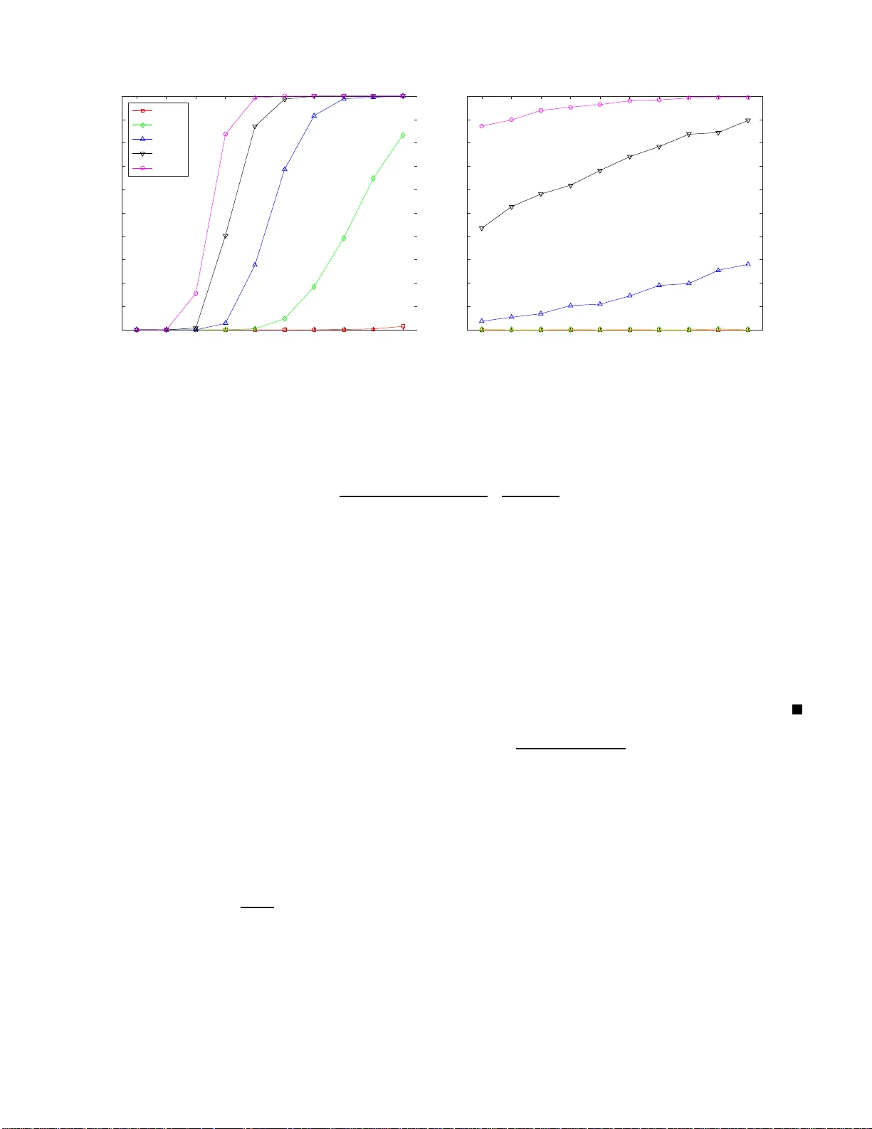
1 Adv ersarial T op- K Ranking Changho Suh V incent Y . F . T an Renbo Zhao Abstract W e study the top- K ranking prob lem wher e the goal is to recover the set of top- K ranked items out of a large collection of items based on pa rtially r ev ealed preferenc es. W e consider an adversarial cr owdsour ced setting where there are two pop ulation sets, and pairwise comparison sam ples d rawn fro m on e of the populations follow the standard Bradley-T er ry-Lu ce mode l (i.e., the chan ce of item i b eating item j is proportion al to the relati ve score of item i to item j ), while in the oth er po pulation, the co rrespon ding chance is inversely p ropor tional to the relati ve score. When the relative size of the two popula tions is known, we characterize th e minimax limit on the samp le size required (up to a co nstant) for reliably id entifying the top- K items, and demonstrate ho w it scales with the relativ e size. Moreover , by leveraging a tensor decomp osition method for disambigu ating mixture distributions, we extend our r esult to the mo re r ealistic scenario in which the relativ e pop ulation size is u nknown, thus establishing an uppe r bound on th e funda mental limit of th e sample size for recovering the top- K set. Index T er ms Adversarial pop ulation, Bradley-T er ry-Lu ce model, crowdsourcing , minimax o ptimality , sample co mplexity , top - K rankin g, tensor decom positions I . I N T R O D U C T I O N Ranking is o ne of the fundamental problems tha t ha s proved crucial in a wide vari ety of co ntexts—social choice [1], [2], web search and information retri ev al [3], rec ommenda tion sy stems [4], ranking indi viduals by group comparisons [5] and crowdsourcing [6], to na me a few . Due to its wide applicability , a lar ge v olume of work on ranking has been done. The two main paradigms in the literature include spec tral r anking algorithms [3], [7], [8] and maximum likelihood estimation (MLE) [9]. While thes e ranking sch emes yield re asonab ly goo d estimates which are faithful globally w .r .t. the latent preferences (i.e., lo w ℓ 2 loss), it is not n eces sarily guaran teed that this results in o ptimal ranking a ccuracy . Accurate ranking ha s more to do with how well the ordering of the estimates matches that of the true preferen ces (a discrete/combinatorial optimization problem), a nd less to do with how well we can estimate the tr ue preferences (a c ontinuous op timization problem). In ap plications, a ranking algo rithm that ou tputs a total ordering of all the items is not o nly overkill, but it a lso unnece ssarily increa ses complexity . O ften, we pay attention to o nly a few signiﬁcant items. Thus, recent work such as tha t by Ch en a nd S uh [10] s tudied the top - K identiﬁcation tas k. He re, on e aims to recover a correct set of top-ranked items only . This work charac terized the minimax limit o n the sa mple size required (i.e., the sa mple complexity) for reliable top- K ranking, assuming the Bradley-T erry-Luce (BTL) model [11], [12 ]. While this result is c oncerne d with practical issues, there a re still li mitations when modeling other realisti c scena rios. The BTL model c onsidered in [10] assumes that the qua lity of pairwise comp arison information which forms the bas is of the model is the same across anno tators. In reality (e.g., c rowdsourced settings), ho wev er , the quality of the information can vary signiﬁca ntly across different annotators. For instance , there may be a non- negligible fraction of spammers who p rovide ans wers in an adv ersarial manne r . In the c ontext of ad versarial web search [13], web con tents can be maliciously manipulated by spammers for commercia l, soc ial, or political beneﬁts in a robust manner . Alternati vely , there may exist false information such a s f alse v oting in social ne tworks and fake ratings in recommendation systems [14 ]. As an initial e ff ort to add ress this challenge , we in vestigate a so -called adversarial BTL model, which po stulates the existence of two s ets of populations—the faithful a nd ad versarial populations, e ach of which has proportion C. Suh is with the School of Electrical Enginee ring at K orea Advanc ed Institute of Science and T echnology (email: chsuh@kaist.ac.kr). V . Y . F . T an is with the Department of Electrical and Computer Engineering and the Department of Mathematics, National Univ ersity of Singapore. (email: vtan@nus.edu .sg). R. Zhao is with the Department of Electrical and Computer Engineering, National University of S ingapore. (email: elezren@nus.ed u.sg). C. Suh is supported by a gift from Samsung . V . Y . F . T an and R. Zhao gratefully ackno wledge ﬁnancial support from the National Univ ersity of Singapo re (NUS) under the NUS Y oung In v estigator A ward R-263-000-B37-133. 2 η a nd 1 − η res pectively . Speciﬁca lly we consider a BTL-ba sed pairwise co mparison model in which there exist latent variables ind icating ground-truth p reference scores of items. In this mod el, it is assume d that c omparison samples drawn from the faithful pop ulation follow the stand ard BTL model (the probability of item i beating item j is proportional to item i ’ s relativ e s core to item j ), and those of the a dversarial popu lation act in a n “ oppos ite” manner , i.e., the probability of i beating j is in versely proportional to the relati ve sc ore. See Fig. 1. A. Main c ontributions W e s eek to charac terize t he fundamen tal li mits on the s ample size required for top- K ranking, and to dev elop computationally e fﬁcient rank ing algorithms. There are two ma in c ontrib utions in this pape r . Building upon Rank Centrality [7] and SpectralMLE [10], we develop a ranking algorithm to ch aracterize the minimax limit required for top- K ran king, up to co nstant factors, for the η -known sce nario. W e a lso show the minimax optimality of our ran king sc heme b y proving a co n v erse o r imposs ibility res ult that a pplies to a ny ranking algorithm using information-t heoretic methods . As a result, we ﬁnd that the s ample complexity is in versely proportional to (2 η − 1) 2 , wh ich sug gests that less distinct the p opulation siz es, the lar ger the sample complexity . W e also de monstrate that o ur result rec overs that of the η = 1 case in [10], s o the work contained herein is a strict generalization of that in [ 10]. The seco nd contributi on is to estab lish an up per boun d on the sa mple complexity for the mo re prac tically-rele v ant scena rio whe re η is unk nown. A novel proced ure b ased on te nsor decompos ition app roaches in J ain-Oh [15] and Anandku mar e t al. [16] is p roposed to ﬁrst obtain an estimate of the parame ter η that is in a neighb orhood of η , i.e., we see k to obtain an ε -globa lly optimal s olution. This is usually not guaran teed by traditional i terati ve methods suc h as Expectation Maximization [17] . Subsequently , the es timate is the n used in the ran king algorithm that a ssumes knowledge of η . W e de monstrate tha t this algorithm leads to an order-wise worse sample complexity relati ve to the η -known ca se. Our theoretical analys es s ugges t that the degradation is unav oidable if we employ this na tural two-step proc edure. B. Related wor k The most relev ant related works are those b y Che n and Suh [10], Negahba n et al. [7], and Che n et al. [6]. Chen and Suh [10] focused on top- K identiﬁcation under the standard BTL model, and deri ved an ℓ ∞ error bound on preference scores which is intimately related to top- K ranking ac curacy . N egahban et a l. [7] considered the same comparison model and deriv ed an ℓ 2 error bound. A key distinction in our work is that we con sider a dif ferent measureme nt model in wh ich there are two pop ulation sets , a lthough the ℓ ∞ and ℓ 2 norm error analyses in [7], [10] play crucial roles in determining t he sa mple comp lexity . The s tatistical mode l introduc ed by Chen et al. [6] attempts to repre sent c rowdsourced s ettings an d forms the basis of ou r adversarial comparison model. W e note tha t no theoretical an alysis of the s ample complexity is av ailable in [6] o r other related works on c rowdsourced rankings [18]–[20]. For example, Kim et al. [20] employed variational EM-based algo rithms to e stimate the latent sc ores; global o ptimality gu arantees for such algo rithms are dif ﬁcult to establish. Jain and Oh [15] developed a tenso r decompos ition method [16] for learning the parameters of a mixture model [21]–[23] that includes ou r model a s a s pecial cas e. W e s pecialize their mo del and rele v ant results to our setting for determining the a ccuracy of the es timated η . This allows us to e stablish an u pper bound o n the samp le complexity when η is u nknown. Recently , Sha h and W ainwright [24] s howed that a simple c ounting method [25 ] achieves order-wise optimal sample complexity for top- K ranking under a general c omparison model whic h includes, as sp ecial cases, a variety of parametric ranking models including the one unde r co nsideration in this paper (the BTL model). Howev er , the authors made as sumptions on the statistics of the pairwise c omparisons which are different from that in our mode l. Hence, their result is not directly a pplicable to our setting. C. N otations W e provide a brief summary of the notations used throughout the pap er . Let [ n ] represen t { 1 , 2 , · · · , n } . W e denote by k w k , k w k 1 , k w k ∞ the ℓ 2 norm, ℓ 1 norm, and ℓ ∞ norm of w , respec ti vely . Additionally , for any two sequen ces f ( n ) a nd g ( n ) , f ( n ) & g ( n ) or f ( n ) = Ω( g ( n )) mean tha t there exists a (universal) cons tant c suc h 3 F A ITH FUL P OP ULATION A DVE RSA RIAL P OP ULATION A B η 1 − η score vector w Y :=  Y ( ℓ ) ij  ( i, j ) ∈ E pai rw ise samp le 1 2 3 4 top-K r a nkin g ˆ S K Y ( ℓ ) ij ∼ Bern  w i w i + w j  ℓ ∈ A w.p. η Y ( ℓ ) ij ∼ Bern  w j w i + w j  ℓ ∈ B w.p. 1 − η ψ ( · ) Fig. 1. Adversarial top- K ranking gi ven samples Y = { Y ( ℓ ) ij } where ( i, j ) ∈ E and E is the edge set of an Erd ˝ os-R ´ enyi random graph. that f ( n ) ≥ cg ( n ) ; f ( n ) . g ( n ) or f ( n ) = O ( g ( n )) me an that t here exists a co nstant c s uch that f ( n ) ≤ cg ( n ) ; and f ( n ) ≍ g ( n ) or f ( n ) = Θ ( g ( n )) mean that there exist cons tants c 1 and c 2 such that c 1 g ( n ) ≤ f ( n ) ≤ c 2 g ( n ) . The no tation p oly( n ) denotes a sequen ce in O ( n c ) for some c > 0 . I I . P R O B L E M S E T U P W e now des cribe the model which we will analyze subseq uently . W e assu me that the observations used to lea rn the rankings a re in the form o f a limited number of pairwise co mparisons over n items. In an a ttempt to reﬂect the adversarial crowdsourced s etting of our interest in which there a re two population sets—the fait hful and ad versarial sets—we adopt a co mparison model introduce d by Chen et al. [6]. Th is is a gene ralization of the BTL mode l [11], [12]. W e de lve into the details of the componen ts of the model. Pr efer ence scor es: As in the s tandard BTL mo del, this model pos tulates the existence of a ground -truth preference score vector w = ( w 1 , w 2 , . . . , w n ) ∈ R n + . Each w i represents the underlying preference s core of it em i . W ithout loss of generality , we assume that the scores are in non-increa sing o rder: w 1 ≥ w 2 ≥ . . . ≥ w n > 0 . (1) It is assumed that the dynamic rang e of the score vec tor is ﬁx ed irrespectiv e of n : w i ∈ [ w min , w max ] , ∀ i ∈ [ n ] , (2) for some p ositi ve c onstants w min and w max . In fact, the cas e in which t he ratio w max w min grows with n can be readily translated into the above setting by ﬁrst s eparating ou t thos e items with vanishing sc ores (e.g., v ia a simple vot ing method like Borda count [25], [26]). Comparison graph: Let G := ([ n ] , E ) be the c omparison graph such that items i an d j are compared by an annotator if the node pa ir ( i, j ) be longs to the e dge set E . W e will ass ume throughout that the edge se t E is drawn in accordan ce to the Erd ˝ os-R ´ enyi (ER) model G ∼ G n,p . That is node pa ir ( i, j ) app ears inde pende ntly of any o ther node pair with an observati on probability p ∈ (0 , 1) . P a irwise compariso ns: For eac h ed ge ( i, j ) ∈ E , we o bserve L comparison s between i and j . Each outco me, indexed by ℓ ∈ [ L ] and d enoted by Y ( ℓ ) ij , is drawn from a mixture of Be rnoulli distributions weighted by an u nknown parameter η ∈ (1 / 2 , 1] . The ℓ -th o bservation of edg e ( i, j ) has distribution Bern ( w i w i + w j ) with proba bility η and distrib ution Bern ( w j w i + w j ) with probability 1 − η . Hence, Y ( ℓ ) ij ∼ Bern  η w i w i + w j + (1 − η ) w j w i + w j  . (3) See Fig. 1 . When η = 1 / 2 , all the observations are fair coin tos ses. In this case, n o information c an be gleaned about the rankings . Thu s we exclude this degenerate setting from o ur study . The ca se o f η ∈ [0 , 1 / 2) is equi valent 4 to the “mirrored” case of 1 − η ∈ (1 / 2 , 1] where we ﬂip 0 ’ s to 1 ’ s and 1 ’ s to 0 ’ s. So without los s of gen erality , we assume tha t η ∈ (1 / 2 , 1] . W e allo w η to depend on n . Conditioned on the gra ph G , the Y ( ℓ ) ij ’ s are indepe ndent and identically distrib uted across a ll ℓ ’ s, each according to the distrib ution of (3). The c ollection of suf ﬁcient statistics is Y ij := 1 L L X ℓ =1 Y ( ℓ ) ij , ∀ ( i, j ) ∈ E . (4) The per-edge numb er of samples L is measure of the qua lity of the meas urements. W e let Y i := { Y ij } j :( i,j ) ∈E , ~ Y ij := { Y ( ℓ ) ij : ℓ ∈ [ L ] } an d Y := { Y ij } ( i,j ) ∈E be various statistics of the available data. P e rformanc e metric: W e are interested in recoveri ng the top- K ranked items in the collection of n items from the data Y . W e deno te the true s et of top- K ra nked items b y S K which, by our ordering a ssumption, is the set [ K ] . W e would lik e to design a ranking scheme ψ : { 0 , 1 } |E |× L →  [ n ] K  that maps from the a v ailable me asuremen ts to a set of K indices. Given a ranking scheme ψ , the performanc e metric we consider is the pr obability of err or P e ( ψ ) := Pr [ ψ ( Y ) 6 = S K ] . (5) W e co nsider the fundame ntal admiss ible r e g ion R w of ( p, L ) pa irs in which top- K ranking is feasible for a gi ven w , i.e., P e ( ψ ) can b e arbitrarily small for large enough n . In particular , we are interested in the sample c omplexity S δ := inf p ∈ [0 , 1] ,L ∈ Z + sup a ∈ Ω δ  n 2  pL : ( p, L ) ∈ R a  , (6) where Ω δ := { a ∈ R n : ( a K − a K +1 ) /a max ≥ δ } . Here we cons ider a minimax scenario in which, gi v en a s core estimator , nature can behave in an adversarial manner , and so she chooses the worst preference score vector t hat maximizes the probability of e rror und er the con straint that the normalized score separation between the K -th a nd ( K + 1) -th items is at leas t δ . Note that  n 2  p is the expecte d n umber of edges of the E R graph so  n 2  pL is the expected number of pairwise sa mples drawn from the model o f our interest. I I I . M A I N R E S U L T S As suggested in [10], a crucial parameter for successful top- K rank ing is the separation between the tw o items near the decision boun dary , ∆ K := w K − w K +1 w max . (7) The sample complexity d epends on w and K only through ∆ K —more precisely , it decrea ses as ∆ K increases . Our c ontributi on is to ide ntify relations hips betwee n η and the sample complexity when η is known and unknown. W e will se e that the sa mple complexity increa ses as ∆ K decreas es. This is intuiti vely true as ∆ K captures how distinguishable the top- K set is from the rest of the items. W e assume that the graph G is drawn from the ER model G n,p with edge appe arance probability p . W e require p to satisfy p > log n n . (8) From ran dom graph theory , this implies that the graph is co nnected with high probab ility . If the graph we re not connec ted, ran kings cann ot be inferr ed [ 9]. W e start by considering the η -known scena rio in which key ingredients for ra nking algorithms an d analysis can be ea sily diges ted, as we ll a s which forms the ba sis for the η -unk nown se tting. Theorem 1 (Known η ) . Suppos e that η is k nown and G ∼ G n,p . Also assume that L = O (p oly( n )) and Lnp ≥ c 0 (2 η − 1) 2 log n . Then with pr obab ility ≥ 1 − c 1 n − c 2 , the set of top- K set ca n be identiﬁed exactly pr ovided L ≥ c 3 log n (2 η − 1) 2 np ∆ 2 K . (9) 5 Con versely , for a ﬁxed ǫ ∈ (0 , 1 2 ) , if L ≤ c 4 (1 − ǫ ) log n (2 η − 1) 2 np ∆ 2 K (10) holds, then for any top- K ranking scheme ψ , ther e exists a pr efer ence ve ctor w with se paration ∆ K such that P e ( ψ ) ≥ ǫ . Here, and i n the following, c i > 0 , i ∈ { 0 , 1 , . . . , 4 } ar e ﬁnite unive rsal constants. Pr oof: See Section IV for the algorithm an d a s ketch of the ac hiev ability proof (suf ﬁciency). The proof of the con verse (imposs ibility part) c an be found in Section V. This theorem a sserts that the samp le complexity scales a s S ∆ K ≍ n log n (2 η − 1) 2 ∆ 2 K . (11) This result recovers that for the faithful sc enario where η = 1 in [10]. When η − 1 2 is u niformly bounde d above 0 , we achieve the sa me order -wise sa mple complexity . This s uggests that the rank ing performance is not sub stantially worsened if the s izes of the two po pulations are sufﬁciently distinct. For the c hallenging s cenario in which η ≈ 1 2 , the sample complexity depe nds on how η − 1 2 scales with n . Indeed , this dep endenc e is q uadratic. T his theo retical result will be validated by expe rimental res ults in Section VII. Se veral other remarks are in order . No c omputational barr ier: Our prop osed algo rithm is ba sed primarily upon two popular ranking a lgorithms: spectral methods and MLE, both of which e njoy nearly-linear time co mplexity in our ranking problem context. Hence, the informati on-theoretic li mit promised by (11) can be achieved by a computationally efﬁcient a lgorithm. Implication of the minimax low er bound: The minimax lower bound con tinues to hold wh en η is unkn own, since we c an only do b etter for the η -known sce nario, a nd he nce the lo wer boun d is also a lo wer bo und in the η -unkn own scena rio. Another adve rsarial sc enario: Ou r results readily gene ralize to another adversarial scenario in which samp les drawn from the a dversarial po pulation are completely noisy , i.e., they follow the distrib ution Bern ( 1 2 ) . W ith a slight modiﬁcation of our p roof tech niques, o ne c an easily verify that the sample comp lexity is on the order of n log n η 2 ∆ 2 K if η is kno wn. This wi ll b e evident after we d escribe the algorithm in Section IV. Theorem 2 (Unknown η ) . Sup pose that η is u nknown and G ∼ G n,p . Also a ssume that L = O (p oly ( n )) and Lnp ≥ c 0 (2 η − 1) 4 log 2 n . The n with pr oba bility ≥ 1 − c 1 n − c 2 , the top- K set can b e identiﬁed exactly pro vided L ≥ c 3 log 2 n (2 η − 1) 4 np ∆ 4 K . (12) Pr oof: Se e Sec tion VI f or the key ide as in the proof. This theorem implies that the sample complexity sa tisﬁes S ∆ K . n log 2 n (2 η − 1) 4 ∆ 4 K . (13) This bou nd is worse than (11) —the in verse d epend ence on (2 η − 1) 2 ∆ 2 K is now an in verse de penden ce on (2 η − 1) 4 ∆ 4 K . This is be cause our algorithm in v olves estimating η , incurring some loss. Whe ther this los s is fun damentally unav oidable (i.e., whether the algorithm is order -wise optimal or not) is open. See detailed d iscussion s in Section VIII. Mo reover , since the estimation of η is ba sed on tensor decompo sitions with polyn omial-time co mplexity , o ur algorithm for the η -unk nown cas e is also, in principle, computationally e f ﬁcient. Note that minimax lower bou nd in (11) also serves as a lower b ound in the η -unk nown sc enario. I V . A L G O R I T H M A N D A C H I E V A B I L I T Y P R O O F O F T H E O R E M 1 A. Algorithm Description Inspired by the con sistency between the p reference s cores w and ranking under the BTL model, our s cheme also adopts a two-step a pproach whe re w is ﬁrst estimated and then the top- K se t is re turned. Recently a top- K rank ing algorithm Spec tralMLE [10] has been developed for the faithful scen ario and it is shown to ha ve order- wise optimal s ample complexity . Th e algorithm yields a small ℓ ∞ loss of the score vector w 6 S PE CTR AL ML E Y sh ift ing ˜ Y R ANK C ENTRALIT Y w ( 0 ) po in t- wis e ML E ˆ w return top - K item s ψ ( Y ) Fig. 2. Ranking algorithm for the η -known scenario: (1) shifting the empirical mean of pairwise measurements to get ˜ Y ij = Y ij − (1 − η ) 2 η − 1 , which con verges to w i w i + w j as L → ∞ ; (2) performing S pectralMLE [10] seeded by ˜ Y to obtain a score estimate ˆ w ; (3) return a ranking based on the estimate ˆ w . Our analysis rev eals that the ℓ ∞ norm bound w .r .t. ˆ w satisﬁes k ˆ w − w k ∞ . 1 2 η − 1 q log n npL , which in t urn ensures P e → 0 und er ∆ K % 1 2 η − 1 q log n npL . which en sures a small point-wise e stimate error . Es tablishing a key relationship between the ℓ ∞ norm e rror and top- K ranking ac curacy , Che n and Suh [10] then ide ntify an order-wise tight bound on the ℓ ∞ norm error requ ired for top- K ranking, thereby characterizing the sa mple complexity . Our ranking algorithm builds on SpectralMLE, which procee ds in tw o stages: (1) an appropriate initialization that conc entrates around the ground truth in an ℓ 2 sense , wh ich can be obtained via spectral methods [3], [7], [8]; (2) a seque nce of T iterati ve updates sharpening the e stimates in a point-wise man ner using MLE. W e o bserve that RankCentrality [7] can be employed as a spectral method in the ﬁrst stage . In fact, RankCentrality exploits the f act that the empiri cal mean Y ij con ver ges to the relative score w i w i + w j as L → ∞ . This motiv ates the use o f the empirical mean for co nstructing the tr ansition probability from j to i o f a Markov ch ain. Note that the detailed ba lance eq uation π i w j w i + w j = π j w i w i + w j that h olds as L → ∞ will enforce that the stationary distrib ution of the Markov ch ain is identical to w up to some con stant scaling. Hence, the stationary d istrib ution is expected to s erve as a reaso nably goo d global score estimate. Howev er , in ou r problem setting where η is not ne cessa rily 1 , the e mpirical mean does not c on ver ge to the relativ e score, instead it be haves as Y ij L →∞ − → η w i w i + w j + (1 − η ) w j w i + w j . (14) Note, howev er , that the limit is linea r in the desired relativ e score and η , implying that knowledge of η leads to the rela ti ve score. A natural idea then a rises. W e co nstruct a shifted version of the empirical me an: ˜ Y ij := Y ij − (1 − η ) 2 η − 1 L →∞ − → w i w i + w j , (15) and take this as an inpu t to Ran kCentrality . This then forms a Markov chain that yields a stationary dis trib ution that is proportional to w as L → ∞ and hence a good es timate of the groun d-truth sco re vector whe n L is large. This se rves a s a g ood initial e stimate to the se cond stage of Spec tralMLE as it guarantee s a small point-wise error . A formal and more detailed description of the proce dure is su mmarized in Algorithm 1. For completen ess, we also include the proce dure of Ra nkCentrality in Algorithm 2. Here we emphas ize tw o d istinctions w .r .t. the se cond stage o f Sp ectralMLE . First, the compu tation of the p ointwise MLE w .r .t. say , it em i , requires knowledge of η : L  τ , w ( t ) \ i ; Y i  = Y j :( i,j ) ∈E "  η τ τ + w ( t ) j + (1 − η ) w ( t ) j τ + w ( t ) j  Y ij  η w ( t ) j τ + w ( t ) j + (1 − η ) τ τ + w ( t ) j  1 − Y ij # . (16) Here, L ( τ , w ( t ) \ i ; Y i ) is the proﬁle likelihood o f the p reference s core vector [ w ( t ) 1 , · · · , w ( t ) i − 1 , τ , w ( t ) i +1 , · · · , w ( t ) n ] where w ( t ) indicates the preferen ce sco re estimate in the t -th iteration, w ( t ) \ i denotes the sco re estimate exclud ing the i -th compone nt, and Y i is the d ata a v ailable at node i . The seco nd difference is the use of a dif ferent thresho ld ξ t which incorporates the ef fect of η : ξ t := c 2 η − 1 ( s log n npL + 1 2 t s log n pL − s log n npL !) , (17) 7 Algorithm 1 Ad versarial top- K ranking for the η -known scenario Input : The a verage c omparison outco me Y ij for all ( i, j ) ∈ E ; the s core ran ge [ w min , w max ] . Partition E ran domly into tw o s ets E init and E iter each containing 1 2 |E | edges. Denote by Y init i (resp. Y iter i ) the compone nts of Y i obtained over E init (resp. E iter ). Compute the shifted version of the average compa rison output: ˜ Y ij = Y ij − (1 − η ) 2 η − 1 . Denote by ˜ Y init i the compone nts of ˜ Y i obtained o ver E init Initialize w (0) to be the es timate computed b y R ank Centrality on ˜ Y init i ( 1 ≤ i ≤ n ). Succes sive Re ﬁnement: f or t = 0 : T do 1) Comp ute the coordinate-wise MLE w mle i ← arg max τ L  τ , w ( t ) \ i ; Y iter i  where L is the li kelihood function deﬁned in (16). 2) For each 1 ≤ i ≤ n , set w ( t +1) i ← ( w mle i , | w mle i − w ( t ) i | > ξ t ; w ( t ) i , else, where ξ t is the replacement thresho ld deﬁn ed in (17). Output the indice s of the K largest c ompone nts of w ( T ) . Algorithm 2 Ra nk Centrality [7] Input : The shifted average c omparison outco me ˜ Y ij for all ( i, j ) ∈ E iter . Compute the transition matrix ˆ P = [ ˆ p ij ] 1 ≤ i,j ≤ n such that for ( i, j ) ∈ E iter ˆ p ij = ( ˜ Y ji d max , if i 6 = j ; 1 − 1 d max P k :( i,k ) ∈E iter ˜ Y k i , if i = j. where d max is the maximum out-degrees of v ertices in E iter . Output the stationary distribution of ˆ P . where c > 0 is a c onstant. This thresh old is use d to decide whether w ( t +1) i should be s et to b e the po intwise MLE w mle i in (22) (if | w mle i − w ( t ) i | > ξ t ) or remains as w ( t ) i (otherwise). The design of ξ t is bas ed on (1) the ℓ ∞ loss incurred in the ﬁrst stage; and (2) a desirable ℓ ∞ loss that we intend to ac hiev e at the end of the se cond stag e. Since these two values are dif ferent, ξ t needs to b e adap ted acco rdingly . Notice that the computation of ξ t requires knowledge of η . The two mo diﬁcations in (16) and (17) result in a more complicated a nalysis vis- ` a-vis Ch en a nd Suh [10]. B. Achievability Pr oof of Theor em 1 Let ˆ w be the ﬁnal estimate w ( T ) in the second stage. W e carefully analyze the ℓ ∞ loss of the w vector , showing that un der the conditions in T heorem 1 k ˆ w − w k ∞ ≤ c 1 2 η − 1 s log n npL . (18) holds with probability exce eding 1 − c 2 n − c 3 . This bo und together with the following observation completes the proof. Obse rve that if w K − w K +1 ≥ c 4 2 η − 1 q log n npL , then f or a top - K item 1 ≤ i ≤ K and a non-top- K item 8 j ≥ K + 1 , ˆ w i − ˆ w j ≥ w i − w j − | w i − ˆ w i | − | w j − ˆ w j | (19) ≥ w K − w K +1 − 2 k ˆ w − w k ∞ > 0 . (20) This implies that o ur ranking algorithm outputs the top - K ranked items a s des ired. Hence , as lon g as w K − w K +1 % 1 2 η − 1 q log n npL holds (coinciding with the c laimed bound in T heorem 1), we ca n guarantee perfect top- K ranking , which co mpletes the proof of Theorem 1. The remaining part is the proof of (18). The proof builds upon the analysis made in [10], which demonstrates the relationship betwee n k w (0) − w k k w k and k w ( T ) − w k ∞ . W e establish a new relationship for the arbitrary η case, formally stated in the foll owi ng lemma. W e will then us e this to prove (18 ). Lemma 1. F ix δ, ξ > 0 . Consider ˆ w ub such that it is inde penden t of G and satisﬁe s k ˆ w ub − w k k w k ≤ δ and k ˆ w ub − w k ∞ ≤ ξ . (21) Consider a n estimate of the s core vector ˆ w such that | ˆ w i − w i | ≤ | ˆ w ub i − w i | for all i ∈ [ n ] . Le t w mle i := arg max τ L ( τ , ˆ w \ i ; Y i ) . (22) Then, the pointwise error | w mle i − w i | ≤ c 0 max ( δ + log n np · ξ , c 1 2 η − 1 s log n npL ) (23) holds with pr o bability at least 1 − c 2 n − c 3 . Pr oof: The relationship in the faithful sc enario η = 1 , wh ich was proved i n [10], me ans that the p oint-wise MLE w mle i is close to the ground truth w i in a compo nent-wise manner , once an initial e stimate ˆ w is accu rate enough . Unlike the faithful sc enario, in our s etting, we h ave (in ge neral) noisier mea surements Y i due to the eff ect of η . Nonethe less this lemma re veals that the relationship for the case of η = 1 is almos t the same as that for an arbitrary η c ase only with a slight modiﬁc ation. This implies that a s mall point-wise loss is still guaran teed as long as we s tart from a reasonably good es timate. Here the only difference in the relationship is that the multi plication term of 1 2 η − 1 additionally app lies in the upper bo und of (23). See Ap pendix A for the proof. Obviously the accuracy o f the point-wise MLE reﬂe cted in the ℓ ∞ error depen ds c rucially on an initial error k w (0) − w k . In fact, Lemma 1 lea ds to the claimed bound (18) onc e the initial estimation e rror is properly chosen as follows: k w (0) − w k k w k . 1 2 η − 1 s log n npL . (24) Here we demonstrate that the desired initial estimation error can indeed be achieved in ou r problem setting, formally stated in L emma 2 (see below). On the other h and, ad apting the ana lysis in [10], one can verify that with the rep lacement thresho ld ξ t deﬁned in (17), the ℓ 2 loss is monotonically decreas ing in a n order-wise se nse, i.e., k w ( t ) − w k k w k . k w (0) − w k k w k . (25) W e are now ready to prove (18) when L = O (p oly( n )) and k w ( t ) − w k k w k ≍ δ ≍ 1 2 η − 1 s log n npL . (26) Lemma 1 asserts that in this regime, t he point-wise MLE w mle is expe cted to satisfy k w mle − w k ∞ . k w ( t ) − w k k w k + log n np k w ( t ) − w k ∞ . (27) 9 Using the analysis in [10], one ca n show that the choice of ξ t in (17) e nables us to detect outliers (whe re an estimation error is large) an d drag down the co rresponding point-wise error , thereby ensu ring that k w ( t +1) − w k ∞ ≍ k w mle − w k ∞ . Th is togethe r with the fact that k w ( t ) − w k k w k . k w (0) − w k k w k . 1 2 η − 1 s log n npL (28) (see (26) above and Le mma 2) gi ves k w ( t +1) − w k ∞ . 1 2 η − 1 s log n npL + log n np k w ( t ) − w k ∞ . (29) A straightforward c omputation with this recursion yields (18) if log n np is sufﬁciently small (e.g., p > 2 log n n ) and T , the n umber of iterations in the second s tage of SpectralMLE , is suf ﬁciently lar ge ( e.g., T = O (log n ) ). Lemma 2. Let L = O (p oly( n )) and Lnp ≥ c 0 (2 η − 1) 2 log n . Let w (0) be an initial estimate: an output of RankCen- trality [7] when se eded by ˜ Y := { ˜ Y ij } ( i,j ) ∈E . Th en, k w − w (0) k k w k ≤ c 1 2 η − 1 s log n npL (30) holds with pr o bability exceeding 1 − c 2 n − c 3 . Pr oof: Here we provide only a sketch of the p roof, le aving details to Appe ndix B. Th e proof builds u pon the analysis structured by Lemma 2 in Negahb an et a l. [7], which bounds the deviation of the Ma rkov chain w .r .t. the transition matrix ˆ P after t steps: k ˆ p t − w k k w k ≤ ρ t k ˆ p 0 − w k k w k r w max w min + 1 1 − ρ k ∆ k r w max w min (31) where ˆ p t denotes the d istrib ution w . r .t. ˆ P at time t see ded by an arbitrary initial distrib ution ˆ p 0 , the matrix ∆ := ˆ P − P , indicates the ﬂu ctuation of the transition probability matrix 1 around its mea n P := E [ ˆ P ] , and ρ := λ max + k ∆ k q w max w min . He re λ max = max { λ 2 , − λ n } and λ i indicates the i -th eigenv alue of P . Unlike the f aithful sce nario η = 1 , in the arbitrary η case, the b ound on k ∆ k depend s on η : k ∆ k . 1 2 η − 1 s log n npL , (32) which will be p roved in Lemma B by us ing various concentration bounds (e.g., Hoeffding and T ropp [27]). Adapting the analysis in [7], one can easily verify that ρ < 1 unde r one of the conditions in Theorem 1 tha t Ln p % log n (2 η − 1) 2 . Applying the bound on k ∆ k and ρ < 1 to (31) giv es the c laimed bo und, which completes the proo f. V . C O N V E R S E P RO O F O F T H E O R E M 1 As i n Chen and Suh’ s work [10], by Fano’ s ine quality , we see tha t it suf ﬁces for us to upper b ound the mutual information between a set of appropriately ch osen rank ings M of cardinality M := min { K, n − K } + 1 . More speciﬁca lly , let σ : [ n ] → [ n ] represen t a permutation over [ n ] . W e also denote by σ ( i ) an d σ ([ K ]) the correspo nding index of the i -th ranked item and the index se t of all top- K items, respe ctiv ely . W e subs equently impo se a uniform prior over M a s follows: If K < n/ 2 t hen Pr( σ ([ K ]) = S ) = 1 M for S = { 2 , . . . , K } ∪ { i } , i = 1 , K + 1 , . . . , n (33) and if K ≥ n / 2 , then Pr( σ ([ K ]) = S ) = 1 M for S = { 1 , . . . , K + 1 } \ { i } , i = 1 , . . . , K + 1 . (34) 1 The notation ∆ = ˆ P − P , a matrix, should not be confused with the scalar normalized score separation ∆ K , deﬁned in ( 7). 10 In words, e ach alternative hypothes is is gene rated by swapping o nly two indice s of the hyp othesis (ranking) obeying σ ([ K ]) = [ K ] . Clearly , the original minimax error probability is lo wer bound ed by the correspond ing error proba bility of this reduced e nsemble. Let the set of observations for the edge ( i, j ) ∈ E be denoted as ~ Y ij := { Y ( ℓ ) ij : ℓ ∈ [ L ] } . W e also ﬁnd it con venient to introduce an erased version of the ob servations Z = { ~ Z ij : i, j ∈ [ n ] } which is related to the true observations Y := { ~ Y ij : ( i, j ) ∈ E } as follows, ~ Z ij =  ~ Y ij ( i, j ) ∈ E e ( i, j ) / ∈ E . (35) Here e is an erasu r e symb ol. Let σ , a chanc e variable, be a uniformly distri buted ranking in M (t he ensemble of rankings crea ted in (33)–(34)). Let P ~ Y ij | σ j be the distribution of the obse rvati ons gi ven that the ranking is σ j ∈ M where j ∈ [ M ] an d a similar notation is used for when ~ Y ij is replaced by ~ Z ij . No w , by the con vexit y of the relati ve entropy and the fact that the rankings a re u niform, the mutual information c an be bounded as I ( σ ; Z ) ≤ 1 M 2 X σ 1 ,σ 2 ∈M D  P Z | σ 1   P Z | σ 2  (36) = 1 M 2 X σ 1 ,σ 2 ∈M X i 6 = j D  P ~ Z ij | σ 1   P ~ Z ij | σ 2  (37) = p M 2 X σ 1 ,σ 2 ∈M X i 6 = j D  P ~ Y ij | σ 1   P ~ Y ij | σ 2  (38) = p M 2 X σ 1 ,σ 2 ∈M X i 6 = j L X ℓ =1 D  P Y ( ℓ ) ij | σ 1   P Y ( ℓ ) ij | σ 2  . (39) Assume that under ranking σ 1 , the score vector is w := ( w 1 , . . . , w n ) an d und er ranking σ 2 , the score vector is w ′ := ( w π (1) , . . . , w π ( n ) ) for some ﬁxed p ermutation π : [ n ] → [ n ] . By us ing the statistical model des cribed in Section II, we know that D  P Y ( ℓ ) ij | σ 1   P Y ( ℓ ) ij | σ 2  = D  η w i w i + w j + (1 − η ) w j w i + w j    η w π ( i ) w π ( i ) + w π ( j ) + (1 − η ) w π ( j ) w π ( i ) + w π ( j )  (40) where D ( α k β ) := α log α β + (1 − α ) log 1 − α 1 − β is the binary relati ve entropy . For brevity , write a := w i w i + w j , and b := w π ( i ) w π ( i ) + w π ( j ) . (41) Furthermore, we note tha t the c hi-squared di ver gence is an upper bound f or the relati ve entropy between tw o distrib utions P = { P i } i ∈X and Q = { Q i } i ∈X on the same (countab le) alphabet X (see e.g. [28 , Lemma 6.3]), i.e., D ( P k Q ) ≤ χ 2 ( P k Q ) := X i ∈X ( P i − Q i ) 2 Q i . (42) W e also use the notation χ 2 ( α k β ) to denote the binary chi-squared diver gence similarly to the binary relative entropy . Now , we may bound (40 ) us ing the follo wing computation D  η a + (1 − η )(1 − a )   η b + (1 − η )(1 − b )  ≤ χ 2  η a + (1 − η )(1 − a )   η b + (1 − η )(1 − b )  (43) = (2 η − 1) 2 ( a − b ) 2  (2 η − 1) b + (1 − η )  η − (2 η − 1) b  (44) Now | a − b | ≤ w K w K + w K +1 − w K +1 w K + w K +1 ≤ w max 2 w min ∆ K . (45) Hence, if we c onsider the case where η = (1 / 2 ) + (which is the re gime of interes t), uniting (44 ) and (45) we ob tain D  η a + (1 − η )(1 − a )   η b + (1 − η )(1 − b )  . (2 η − 1) 2 ∆ 2 K . (46) 11 By construction of the hyp otheses in (33)–(34), c onditional on any two d istinct ran kings σ 1 , σ 2 ∈ M , the d istrib u- tions o f ~ Y ij (namely P ~ Y ij | σ 1 and P ~ Y ij | σ 2 ) are dif ferent over at most 2 n locations so X i 6 = j L X l =1 D  P Y ( ℓ ) ij | σ 1   P Y ( ℓ ) ij | σ 2  . nL (2 η − 1) 2 ∆ 2 K . (47) Thus, plugg ing this into the bound o n the mutual information in (39), we ob tain I ( σ ; Z ) . pnL (2 η − 1) 2 ∆ 2 K . (48) Plugging this into Fano’ s inequality , and u sing the fact that M ≤ n/ 2 (from M = min { K, n − K } + 1 ), we obtain P e ( ψ ) ≥ 1 − I ( σ ; Z ) log M − 1 log M (49) ≥ 1 − I ( σ ; Z ) log( n/ 2) − 1 log( n / 2) . (50) Thus, if S =  n 2  pL ≤ c 2 (1 − ǫ ) log n (2 η − 1) 2 ∆ 2 K for some small enou gh but p ositi ve c 2 , we see that P e ( ψ ) ≥ ǫ. (51) Since this is indep enden t of t he decoder ψ , the con verse pa rt is prov ed. V I . A L G O R I T H M A N D P RO O F O F T H E O R E M 2 A. Algorithm Description The proof of Theorem 2 follows b y combining the res ults o f Jain and Oh [15] with the analysis for the case when η is kn own in Th eorem 1 . J ain and Oh were interested in d isambiguating a mixture dis trib ution from samples. This corresponds to our mo del in (3). They showed using tens or decomposition metho ds that it is po ssible to ﬁnd a globally op timal so lution for the mixture we ight η using a c omputationally efﬁcient algorithm. They a lso provided an ℓ 2 bound on the error of the distributions but as mentioned, we are more interested in controlling the ℓ ∞ error s o we estimate w sep arately . The use of the ℓ 2 bound in [15] leads to a worse s ample c omplexity for top- K ranking. Thus, in the ﬁrst step, we will us e the method in [15] to estimate η g i ven the data sa mples (pairwise c omparisons) Y . The estimate is deno ted as ˆ η . It turns out tha t one ca n spe cialize the result in [15] with s uitably parametrized “distributi on vec tors” π 0 :=  . . . w i w i + w j w j w i + w j w i ′ w i ′ + w j ′ w j ′ w i ′ + w j ′ . . .  T (52) and π 1 := 1 2 |E | − π 0 ∈ R 2 |E | and where in ( 52), ( i, j ) runs throug h all values in E . Henc e, we are in fact a pplying [15] to a more restricti ve setting where the two probability distributions represented by π 0 and π 1 are “c oupled” but this do es not preclude the application of the results in [15]. In fact, this assumption ma kes the calculation of relev ant p arameters (in Lemma 6) easier . The relevant s econd and thir d moments are M 2 := η π 0 ⊗ π 0 + (1 − η ) π 1 ⊗ π 1 , ( 53) M 3 := η π 0 ⊗ π 0 ⊗ π 0 + (1 − η ) π 1 ⊗ π 1 ⊗ π 1 , (54) where π j ⊗ π j ∈ R (2 |E | ) × (2 |E | ) is the outer product a nd π j ⊗ π j ⊗ π j ∈ R (2 |E | ) × (2 |E | ) × (2 |E | ) is the 3 -fold tensor outer produc t. If one has the exact M 2 and M 3 , we ca n obtain the mixture weight η exactly . The intuition a s to why tensor methods are app licable to problems in v olving latent variables ha s been well-documented (e.g. [16]). Essentially , the second- and third-moments contained in M 2 and M 3 provide suf ﬁcient s tatistics for identifying and hence estimating a ll the parame ters of an a ppropriately-deﬁne d model with latent variables (whereas sec ond-order information c ontained in M 2 is, in ge neral, not sufﬁcient for recon structing the parameters). Thus, the prob lem boils down to analyzing the precision of η when we o nly have access to em pirical versions of M 2 and M 3 formed from pairwise co mparisons in G . As shown in Lemma 5 to foll ow , the re is a tradeo f f between the sa mple s ize per edge L an d the quality of the es timate of η . Hence, this caus es a degradation to the overall sample complexity reﬂected in Theorem 2. 12 Y s hif ting ˜ Y R ANK C ENTRALIT Y w ( 0 ) po in t- wis e ML E ˆ w return top - K item s ψ ( Y ) T ENSOR M ET HO D ˆ η S PE CTR AL ML E Fig. 3. Ranking algorithm for the unkno wn η scenario. The key distinction relativ e to the kno wn η case is that we estimate η based on t he tensor decomposition method [15], [16] and the estimate ˆ η is employed for shifting Y and performing the point-wise MLE . This method allows us to get k ˆ w − w k ∞ . 1 2 η − 1 4 q log 2 n npL , which ensures that P e → 0 und er ∆ K % 1 2 η − 1 4 q log 2 n npL . Algorithm 3 Es timating mixing coef ﬁcient η [15] Input : The collection of observed pairwise comparisons Y Split Y evenly into two subse ts of sa mples Y (1) and Y (2) Estimate the second-order moment ma trix M 2 in (53) based on Y (1) using Algo rithm 2 (Matr ixAltMin) in [15] Estimate a third-or der statistic G (de ﬁned i n [15, Theorem 1]) based on ( M 2 , M 3 , Y (2) ) us ing Algorithm 3 (T ensorLS) in [ 15] Compute the ﬁrst eigenv alue λ 1 of G using the r obust power method in [16] Return the estimated mixing coefﬁcient ˆ η = λ − 2 1 In the second s tep, we p lug the e stimate ˆ η into the algorithm for the η -kn own c ase by sh ifting the o bservations Y similarly to (15) but with ˆ η instead of η . See Fig. 3. Howe ver , he re the re are a couple of important distinctions relati ve to the ca se where η is known exactly . First, the likelihood func tion L ( · ) in (16) nee ds to be modiﬁe d since it is a function o f η in which now we o nly h ave its e stimate ˆ η . Second , since the guarantee o n the ℓ ∞ loss of t he preference score vector w is d if ferent (and in fact worse), we nee d to design the thresh old ξ t dif ferently from (17). W e call the modiﬁed threshold ˆ ξ t , to be deﬁn ed precisely in (58). B. Pr oof o f The orem 2 As i n S ection IV -B, the crux is to ana lyze the ℓ ∞ loss of the w vector . W e s how tha t k ˆ w − w k ∞ ≤ c 0 2 η − 1 4 s log 2 n npL (55) holds with probability ≥ 1 − c 1 n − c 2 . T o g uarantee accurate top- K ranking, we then follo w the same argument as in (19)– (20). W e lower bou nd k ˆ w − w k ∞ in (55) by ∆ K and solve for L . Thus, it s ufﬁces to show (55) un der the conditions of Theorem 2. The proof of (55) follo ws from sev eral lemmata, two of which we pres ent in this se ction. Th ese a re the analogues of Lemmas 1 and 2 for the η -kn own case. Once we have these two lemmata, the strategy to proving (55) is almos t the s ame as that in the η -known setting in Section IV -B so we omit the details. The ﬁrst lemma concerns the relationship between the normalized ℓ 2 error and the ℓ ∞ error when we do not have acce ss to the true mixture weight η , but o nly an estimate of it gi ven via Algorithm 3. 13 Lemma 3. Cons ider ˆ w ub such that it is independ ent of G and satisﬁes (21) . Conside r ˆ w such that | ˆ w i − w i | ≤ | ˆ w ub i − w i | for all i ∈ [ n ] . No w d eﬁne w mle i := arg max τ ˆ L ( τ , ˆ w \ i ; Y i ) , (56) where ˆ L ( · ) is the surr ogate likelihood (cf. (16) ) co nstructed with ˆ η in place of η . Then , for all i , the same pointwise MLE b ound in (23) holds wit h probability ≥ 1 − c 0 n − c 1 . Pr oof: The p roof parallels that of Lemma 1 but is more technical. W e an alyze the ﬁdelity of the estimate ˆ η relati ve to η as a function of L (Lemma 5 ). T his requires the spec ialization of J ain an d Oh [15] to our setting. By proving several continuity stateme nts, we show that the estimated normalized log-likelihood (NLL) 1 L log ˆ L ( · ) is uniformly close to the true NLL 1 L log L ( · ) w . h.p. This l eads us to prove (23 ), which is the same as the η -known case. Th e details are deferred to Appendix C. Similarly to the case w here η is known, we need to subsequen tly control the initial error k w (0) − w k . For the η -known case , this is done in Lemma 2 s o the follo wing lemma is an an alogue of Lemma 2. Lemma 4. A ssume the conditions of Theorem 2 hold. Let w (0) be an initial estimate, i.e ., an output of RankCentrality when s eeded by ˜ Y which con sists of the shifted obs ervations with ˆ η in place of η (cf. (15) ). Then, k w − w (0) k k w k ≤ c 0 2 η − 1 4 s log 2 n npL (57) holds with pr o bability ≥ 1 − c 1 n − c 2 . Pr oof: See Se ction VI-C for a sketch of the proo f an d App endix D for a detailed calculation of an upper bound on the spec tral norm of the ﬂuctua tion matrix, w hich is a key ingredient of the proof of Lemma 4. W e remark tha t (57) is worse than it s η -known counterpa rt in (30 ). In p articular , there is no w a fourth root in verse depe ndenc e o n L (compared to a square root in verse dep endenc e), w hich means we potentially need many more o bservations to dri v e the normalized ℓ 2 error k w − w (0) k k w k down to the same le vel. This los s is present bec ause there is a pena lty incurred in e stimating η via the tensor de composition ap proach, es pecially wh en η is close to 1 / 2 . In the a nalysis, we need to control the Lips chitz constan ts of func tions such as t 7→ 1 2 t − 1 and t 7→ 1 − t 2 t − 1 (see e .g. (15)). Such functions behave b adly ne ar 1 / 2 . In particular , the grad ient diver ges as t ↓ 1 / 2 . W e have endeavored to op timize (57) so that it is a s tight as possible, a t leas t us ing the p roposed me thods. Using Le mmas 3 and 4 and in voking a similar argument as in the η -known sc enario, we can now to p rove (55). One key distinction here lies in the ch oice of the threshold: ˆ ξ t := c 2 ˆ η − 1    4 s log 2 n npL + 1 2 t   4 s n log 2 n pL − 4 s log 2 n npL      . (58) The rationa le beh ind this choice, wh ich is different from (17), is tha t it driv es the initial ℓ ∞ loss (as sociated to the initial ℓ 2 loss in Lemma 4) to approach the desired ℓ ∞ loss in (55). T aking this choice, which we optimized, and adapting the analysis in [10 ] with L emma 3, one can verify tha t the ℓ ∞ loss is mon otonically d ecreas ing in an o rder- wise sense: k w ( t ) − w k k w k . k w (0) − w k k w k similarly to (25). By ap plying Lemma 3 to the regime where L = O (p oly ( n )) and k w ( t ) − w k k w k ≍ δ ≍ 1 2 η − 1 4 s log 2 n npL , (59) we get k w mle − w k ∞ . k w ( t ) − w k k w k + log n np k w ( t ) − w k ∞ . (60) As in the η -known setting, one can show that the replaceme nt threshold ˆ ξ t leads to k w mle − w k ∞ ≍ k w ( t ) − w k ∞ . This togethe r with Lemma 4 gives k w ( t +1) − w k ∞ . 1 2 η − 1 4 s log 2 n npL + log n np k w ( t ) − w k ∞ . (61) 14 A s traightforward computation with this recursion yields the claimed bound a s long as log n np is s ufﬁciently small (e.g., p > 2 log n n ) and T is suf ﬁciently large (e.g ., T = O (log n ) ). This completes the p roof of (55). C. P r oof S ketch of Lemma 4 The proof of Lemma 4 relies on the ﬁd elity of the estimate ˆ η as a f unction of L when we use the tensor decompo sition a pproach by Jain and Oh [15 ] on the problem at hand. Lemma 5 (Fidelity of η estimate) . If the n umber of observations per o bserv ed n ode pair L satisﬁes L % 1 ε 2 log n δ , , (62) then the estimate ˆ η is ε -close to the true v alue η with p r obability excee ding 1 − δ . Pr oof: Th e comp lete proof us ing The orem 3 and Lemma 6 is provided in Section VI-D. W e take δ = n − c 0 (for so me constant c 0 > 0 ) in the sequ el so (62 ) reduces to L % 1 ε 2 log n . A major contrib ution in the prese nt paper is to ﬁnd a “swee t spot” for ε ; if it is chos en too sma ll, k ˆ w − w k ∞ is re duced (improving the estimation error) b ut L increases ( worsening the o verall sa mple complexity). Con versely , if ε is chos en to be too lar ge, the requ irement o n L in (62) is relaxed, but k ˆ w − w k ∞ increases and henc e, the overall sample c omplexity grows (worsens) eventually . Th e es timate in (62) is reminiscent of a C hernoff- Hoeffding bou nd e stimate of the sample size p er edge L re quired to ensure that the average of i.i.d. ran dom variables is ε -close to its mean with probability ≥ 1 − δ . Howe ver , the jus tiﬁcation is more in volved and requires spec ializing Theorem 3 (to follow) to our s etting. Now , we denote the difference matrix ∆ := ˆ P − P in which ˆ η is use d in plac e of η as ˆ ∆ . Now using Lemma 5 , several continuity arguments, a nd so me conce ntration inequa lities, we are able to establish that k ˆ ∆ k . 1 2 η − 1 4 s log 2 n npL (63) with probab ility ≥ 1 − c 1 n − c 2 . The ineq uality (63) is proved in Append ix D. Now simi larly to the proo f of Lemma 1, ρ < 1 under the conditions o f Th eorem 2. Applying the bound on the spectral norm of k ˆ ∆ k in (63) to (31) (which continues to hold in t he η -unkn own setting) completes the proof of Le mma 4. D. P r oof o f Le mma 5 T o prove Lemma 5, we specialize the non-asymptotic bound o n the recovery o f parameters in a mixture model in [15] to our setting; cf. (52). Before stating this, we introduce a few notations. Let the singular value decomposition of M 2 , d eﬁned in (53), be written a s M 2 = U Σ V T where Σ = diag ( σ 1 ( M 2 ) , σ 2 ( M 2 )) an d U ∈ R (2 |E | ) × 2 the matrix con sisting of the left-singular v ectors, is fur ther de compos ed a s U =  (( U (1) ) T ( U (2) ) T . . . ( U ( |E | ) ) T  T . (64) Each submatrix U ( k ) ∈ R 2 × 2 where k denotes a node pair . W e say that M 2 is ˜ µ -block-incoherent if the operator norms for all |E | blocks of U , namely U ( k ) , a re uppe r bound ed as k U ( k ) k 2 ≤ ˜ µ s 2 |E | , ∀ k ∈ E . (65) For M 2 , the smalles t bloc k-incoherent co nstant ˜ µ is known as the block-incoherence of M 2 . W e denote this a s µ ( M 2 ) := in f { ˜ µ : M 2 is ˜ µ -block-inco herent } . Theorem 3 (Ja in and Oh [15]) . F ix an y ε, δ > 0 . Th ere e xists a po lynomial-time algo rithm in |E | , 1 ε and log 1 δ (Algorithm 1 in [15]) such that if |E | % σ 1 ( M 2 ) 4 . 5 µ ( M 2 ) σ 2 ( M 2 ) 4 . 5 (66) 15 0.51 0.52 0.53 0.54 0.55 0.56 0.57 0.58 0.59 0.6 η 0 0.1 0.2 0.3 0.4 0.5 0.6 0.7 0.8 0.9 1 Success rate ∆ K = 0.1 ∆ K = 0.2 ∆ K = 0.3 ∆ K = 0.4 ∆ K = 0.5 (a) 0.91 0.92 0.93 0.94 0.95 0.96 0.97 0.98 0.99 1 η 0 0.1 0.2 0.3 0.4 0.5 0.6 0.7 0.8 0.9 1 Success rate (b) Fig. 4. Success rates across η for (a) η close to 1 / 2 and (b) η cl ose to 1 . and for a larg e enou gh (pe r-edge) sam ple size L s atisfying L % µ ( M 2 ) σ 1 ( M 2 ) 6 |E | 3 min { η , 1 − η } σ 2 ( M 2 ) 9 · log( n/δ ) ε 2 , (67) the e stimate of the mixtur e weight ˆ η is ε -close to the true mixture weigh t η w ith pr obab ility exceeding 1 − δ . It remains to estimate the s calings of σ 1 ( M 2 ) , σ 2 ( M 2 ) an d µ ( M 2 ) . Thes e require calculations bas ed on π 0 , π 1 and M 2 and a re s ummarized in the followi ng cruc ial lemma. Lemma 6. F or a ﬁxe d seque nce of grap hs with |E | edges, σ i ( M 2 ) = Θ( |E | ) , i = 1 , 2 , (68) µ ( M 2 ) = Θ(1) . (69) Pr oof: The proof of this lemma ca n be found in Append ix E. It hinges on the fact that k π 0 k 2 = k π 1 k 2 , as the populations have “ permuted” preferen ce s cores. Now the proof of Lemma 5 is immediate up on substituting (68 ) into (66)–(67). W e then notice that |E | = Θ( n 2 p ) = ω (1) with high proba bility so (66 ) is rea dily satisﬁed . Also µ ( M 2 ) σ 1 ( M 2 ) 6 |E | 3 min { η, 1 − η } σ 2 ( M 2 ) 9 = Θ(1) so we recover (62) as de sired. V I I . E X P E R I M E N T A L R E S U LT S For the cas e where η is k nown, a n umber o f expe riments on synthetic data w ere conduc ted to validate The orem 1. W e ﬁrst s tate parameter s ettings co mmon to all experiments. The total numbe r of items is n = 1000 and the number of ranked items K = 10 . In the po intwise MLE step in Algorithm 1, we se t the number of iterations T = ⌈ log n ⌉ and c = 1 in the formula for the threshold ξ t in (17 ). The observation probability o f each edge of the Erd ˝ os-R ´ enyi g raph is p = 6 log n n . Th e latent scores are uniformly gen erated from the dynamic ra nge [0 . 5 , 1] . Each (empirical) s ucces s rate is averaged over 1000 Mon te Carlo tri als. W e ﬁrst examine the relations between s ucces s rates a nd η for vari ous values of the n ormalized s eparation of the sco res ∆ K ∈ { 0 . 1 , 0 . 2 , . . . , 0 . 5 } . He re we consider two dif ferent scenarios, one b eing such tha t η is close to 1 / 2 and the other being such that η is c lose to 1 . W e s et the number of samples per edg e, L = 1000 for the ﬁrst case and L = 10 for the seco nd. This is because when η is small, more data samples are needed to achieve non-negligible su ccess rates. The results for thes e two sce narios are shown in Figs. 4(a) and 4(b) respe cti vely . For both ca ses, wh en L is ﬁxed, we obs erve as η increase s, the succe ss rates increase a ccordingly . However , the effect of η on succ ess rates is more p rominent when η is close t o 1 / 2 . This is in ac cordanc e to (11) in The orem 1 since 16 0 2 4 6 8 10 12 14 16 18 S norm 0 0.2 0.4 0.6 0.8 1 Success rate η = 0.6 η = 0.7 η = 0.8 η = 0.9 η = 1.0 Fig. 5. Success rates across normalized sample size S norm . 1 / (2 η − 1) 2 has sharp decrease (as η increases) nea r 1 / 2 and a gentler de crease near 1 . Also, suc cess rates inc rease when ∆ K increases . This aga in corroborates (11) wh ich s ays that the sample complexity is p roportional to 1 / ∆ 2 K . Next we e xamine the relations between su ccess rates and normalized s ample s ize S norm := S ∆ K ( n log n ) / [(2 η − 1) 2 ∆ 2 K ] , (70) for η ∈ { 0 . 6 , 0 . 7 , . . . , 1 } . W e ﬁx ∆ K = 0 . 4 in this c ase. Th e results are sh own in Fig. 5. W e o bserve the relations between success rates and S norm are almost the same for a ll η ’ s so the implied cons tant factor in ≍ notation in (11) depend s very we akly on η (if at all). Finally we nume rically exa mine the relation be tween the sample complexity and η . W e ﬁx ∆ K = 0 . 4 and focus on the regime where η is close to 1 / 2 . For ea ch η , we u se the bisec tion method to a pproximately ﬁn d the minimum sample s ize per edge ˆ L that achieves a high succes s rate q th = 0 . 99 . S peciﬁcally , the bisection proce dure terminates when the empirical s ucces s rate ˆ q corresponding to ˆ L satisﬁe s | ˆ q − q th | < ǫ , where ǫ is set to 5 × 10 − 3 . W e repe at such a procedu re 10 times to get an average resu lt ˆ L a v e . W e also compute the resulting stan dard deviation and observe that it is small acros s the 10 indepen dent runs . Deﬁn e the e xpected minimum total sample size ˆ S :=  n 2  p ˆ L a v e . (71) T o ill ustrate the explicit depe ndenc e of ˆ S on η , we further normalize ˆ S to ˆ S norm := ˆ S ( n log n ) / ∆ 2 K , (72) thus isolating the depen dence of minimum total sa mple size on η only . W e the n ﬁt a curve C / (2 η − 1 ) 2 to ˆ S norm , where C is chos en to bes t ﬁt the p oints by optimizing a least-squares -like obje cti ve function. The empirical results (mean and one stand ard deviation) together with the ﬁtted cu rve are shown in Fig. 6. W e observe ˆ S norm depend s on η via 1 / (2 η − 1) 2 almost perfectly up to a constant. Th is corrobo rates our theoretical result in (11), i.e., the reciprocal de pende nce of the samp le complexity on (2 η − 1) 2 . For the case where η is not kno wn, the storage costs turn out to be prohibiti ve even for a mod erate number of items n . He nce, we leav e the implementation of the algorithm for the η -unk nown case to future work. It is likely that one may need to formulate the ran king prob lem in an online manne r [29] or res ort to online methods for performing ten sor dec ompositions [30]–[32]. 17 0.51 0.52 0.53 0.54 0.55 0.56 0.57 0.58 0.59 0.6 η 0 0.5 1 1.5 2 ˆ S norm × 10 4 C (2 η − 1) 2 Fig. 6. Normalized empirical sample size ˆ S norm for η close to 1 / 2 . V I I I . C O N C L U S I O N A N D F U RT H E R W O R K In t his paper , we hav e p rovided an analytical frame work for a ddressing the prob lem of rec overing the top- K ran ked items in a n adversa rial crowdsourced se tting. W e considered two scenarios. First, the prop ortion o f ad versaries 1 − η is known and the seco nd, more c hallenging scenario, is when this parameter is unknown. For the ﬁrst scen ario, we adapted the S pectralMLE [10] and R ankCen trality [7] algorithms to provide an order- wise optimal sample complexity b ound for the total nu mber of meas urements for recovering the exact top- K se t. These results were veriﬁed numerically and the de pende nce of the samp le c omplexity on the reciprocal of (2 η − 1) 2 was corroborated. For the sec ond sce nario, we adapted Jain and Oh ’ s global optimalit y result for disambiguating a mixture of discrete distrib utions [15] to ﬁrst learn η . Su bsequ ently , we plugge d this (inexact) e stimate into the known- η algorithm and utilized a sequen ce o f continuity arguments to ob tain an up per bound on the s ample complexity . This bo und is order- wise worse than the case where η is known, showing that the error induc ed by the estimation of the mixture parameter do minates the ov erall procedure. A few na tural questions res ult from our analys es. 1) Can we close the gap in the sample complexities between the η -known a nd η -unknown scen arios? This seems challenging gi ven that (i ) threshold ˆ ξ t in (58) must not be dependent on parameters that are a ssumed to be unknown suc h a s the weight se paration ∆ K and (ii) the fundame ntal difﬁculty o f obtaining a g lobally o ptimal solution for the fraction o f ad versaries from sa mples that are drawn from a mixture d istrib ution. Th us, we conjecture that if we adopt a two-step approach—ﬁrst estimate η , then p lug this estimate into the η -kn own algorithm—such a loss is unav oidable. This is beca use the ﬁ delity of the estimate of η in Le mma 5 is natural (cf. Chernof f-Hoef fding bound) and does not see m to be o rder- wise i mprov able. Thu s, we opine that a ne w class of algorithms, avoiding the explicit es timation o f η , needs to b e developed to improve the overall sample complexity performance . 2) If closing the gap is dif ﬁ cult, c an we hope to deri ve a co n verse or impos sibility result, explicitly taking into accoun t the fact tha t η is unknown? Our current con verse result assume s that η is k nown, which may be too optimistic for the unknown setting. 3) The tensor dec omposition method [15], [ 16], wh ile being po lynomial time in its parameters, incurs h igh storage cos ts. Hence, in practice, it implementation t o y ield meaning ful e stimates of η is ch allenging. There has bee n some recen t progress on large-scale scalable tenso r decompos ition algorithms in [30]–[32]. In these works, the authors aim t o av oid storing and manipulating lar ge tensors directly . Howe ver , since implementation is no t the focus of the present work, we leave this to future work. 4) Recent work by Sha h and W ainwright [24] ha s sho wn that simple coun ting methods for certain observation models (including the BTL model) a chieve order- wise optimal s ample co mplexities. In the observation model 18 considered the rein, for e ach pair of items i and j , there is a rando m numbe r o f obs ervations R ij that follows a binomial dis trib ution with p arameters L ∈ N and p robability of s ucces s p ∈ (0 , 1) . Notice that the ob servation model in [24] differs from o urs. 5) Lastly , it would be interesting to c onsider o ther c hoice models (e.g., the Plac kett-Luce model [33] studied in [34] and [35]) as well as other comparison grap hs not limited to the ER grap h, as the comparison graph structure af fects the sample complexity s igniﬁcantly , as suggested in [7, Theorem 1]. A P P E N D I X A P RO O F O F L E M M A 1 For eas e of presentation, we will henceforth as sume that w max = 1 since this simply amounts to a rescaling of all the preference score s. T o prove the lemma, it suf ﬁces to sho w that if τ satisﬁes | τ − w i | % max n δ + log n np · ξ , 1 2 η − 1 q log n npL o , the n the correspond ing likelihood function cannot be the point-wise MLE: L ( τ , ˆ w \ i ; y i ) < L ( w i , ˆ w \ i ; y i ) . (A.1) W e start by e v aluating the likelihood f unction w .r .t. the g round-truth s core vector: ℓ ∗ ( τ ) := 1 L log L ( τ , w \ i ; Y i ) (A.2) = X j :( i,j ) ∈E  Y ij log  η τ τ + w j + (1 − η ) w j τ + w j  + (1 − Y ij ) log  η w j τ + w j + (1 − η ) τ τ + w j  . (A.3) The likelihood los s w .r . t. w i and τ is then computed as : ℓ ∗ ( w i ) − ℓ ∗ ( τ ) = X j :( i,j ) ∈E ( Y ij log η w i w i + w j + (1 − η ) w j w i + w j η τ τ + w j + (1 − η ) w j τ + w j ! + (1 − Y ij ) log η w j w i + w j + (1 − η ) w i w i + w j η w j τ + w j + (1 − η ) τ τ + w j !) . (A.4) T a king expectation w .r .t. Y i conditional on G , we g et: E [ ℓ ∗ ( w i ) − ℓ ∗ ( τ ) |G ] = X j :( i,j ) ∈E D  η w i w i + w j + (1 − η ) w j w i + w j     η τ τ + w j + (1 − η ) w j τ + w j  (A.5) ( a ) % n p (2 η − 1) 2 | w i − τ | 2 (A.6) where ( a ) follows from Pinsker’ s inequality ( D ( p k q ) ≥ 2( p − q ) 2 ; see [36, Theorem 2.33] for example) a nd u sing the fact that d i ≍ np when p > log n n . Here d i indicates the degree of n ode i : the number of edge s incident to node i . This sugge sts that the true point-wise MLE of w i strictly dominates that of τ in the mean sense . W e can actually demonstrate that this is the case beyond the mean sense with high probability , as long as | w i − τ | % 1 2 η − 1 q log n npL (our hy pothesis), which is asse rted in the following lemma. Lemma 7. Suppose that | w i − τ | % 1 2 η − 1 q log n npL . Then , ℓ ∗ ( w i ) − ℓ ∗ ( τ ) % n p (2 η − 1) 2 | w i − τ | 2 . (A.7) holds with pr o bability approaching one. Pr oof: Using Bernstein’ s inequa lity formally stated in Le mma 12 (see App endix F), one ca n obtain a lower bound on ℓ ∗ ( w i ) − ℓ ∗ ( τ ) in terms of its expectation E [ ℓ ∗ ( w i ) − ℓ ∗ ( τ ) |G ] , its variance V a r [ ℓ ∗ ( w i ) − ℓ ∗ ( τ ) |G ] , and the maximum value of individual quantities that we sum over . On e can then show that the variance and the ma ximum value are dominated by the expectation under our hy pothesis, thus proving that the lower bou nd is the o rder of the de sired bound as c laimed. For completenes s, we inc lude the detailed proof a t the end o f this a ppendix; see Appendix A-A. 19 Howe ver , whe n running o ur a lgorithm, we d o not have access to the ground truth sco res w \ i . Wh at w e can actually co mpute is ˆ ℓ ( τ ) := 1 L log L ( τ , ˆ w \ i ; Y i ) (A.8) instead of ℓ ∗ ( τ ) . Fortunately , su ch surrogate lik elihoods are sufﬁciently close to the true likelihoods, which we will show in the rest of the proof. From this, we will next demonstrate that (A.1) holds for suf ﬁciently separated τ such that | τ − w i | % max n δ + log n np · ξ , 1 2 η − 1 q log n npL o . As seen from (A.31), one can quan tify the d if ference between ˆ ℓ ( w i ) and ˆ ℓ ( τ ) as ˆ ℓ ( w i ) − ˆ ℓ ( τ ) = X j :( i,j ) ∈E  Y ij log  ( η w i + (1 − η ) ˆ w j )( η ˆ w j + (1 − η ) τ ) ( η τ + (1 − η ) ˆ w j )( η ˆ w j + (1 − η ) w i )  + log  ( τ + ˆ w j )( η ˆ w j + (1 − η ) w i ) ( w i + ˆ w j )( η ˆ w j + (1 − η ) τ )  . (A.9) Using (A.9) and (A.31), we can rep resent the gap between the surrogate loss and the tr ue l oss a s ˆ ℓ ( w i ) − ˆ ℓ ( τ ) − ( ℓ ∗ ( w i ) − ℓ ∗ ( τ )) = X j :( i,j ) ∈E Y ij   log  ( η w i + (1 − η ) ˆ w j )( η ˆ w j + (1 − η ) τ ) ( η τ + (1 − η ) ˆ w j )( η ˆ w j + (1 − η ) w i )  − lo g  ( η w i + (1 − η ) w j )( η w j + (1 − η ) τ ) ( η τ + (1 − η ) w j )( η w j + (1 − η ) w i )  +  log  τ + ˆ w j w i + ˆ w j  + lo g  η ˆ w j + (1 − η ) w i η ˆ w j + (1 − η ) τ  − log  τ + w j w i + w j  − log  η w j + (1 − η ) w i η w j + (1 − η ) τ   . (A.1 0) Using Berns tein’ s ine quality und er our hypothesis a s we did in Lemma 7, one can verify that ˆ ℓ ( w i ) − ˆ ℓ ( τ ) − ( ℓ ∗ ( w i ) − ℓ ∗ ( τ )) . E h ˆ ℓ ( w i ) − ˆ ℓ ( τ ) − ( ℓ ∗ ( w i ) − ℓ ∗ ( τ )) |G i = X j :( i,j ) ∈E g η ( ˆ w j ) (A.11) where g η ( t ) : = η w i + (1 − η ) w j w i + w j  log  ( η w i + (1 − η ) t )( η t + (1 − η ) τ ) ( η τ + (1 − η ) t )( η t + (1 − η ) w i )  − log  ( η w i + (1 − η ) w j )( η w j + (1 − η ) τ ) ( η τ + (1 − η ) w j )( η w j + (1 − η ) w i )  + log  τ + t w i + t  + log  η t + (1 − η ) w i η t + (1 − η ) τ  − log  τ + w j w i + w j  − log  η w j + (1 − η ) w i η w j + (1 − η ) τ  . (A.12) Here the function g η ( t ) obeys the follo wing two prope rties: (i) g η ( w j ) = 0 and (ii)     ∂ g η ( t ) ∂ t     = (2 η − 1) | τ − w i | ( η t + (1 − η ) τ )( ηt + (1 − η ) w i ) ×     η w i + (1 − η ) w j w i + w j η (1 − η )( t 2 − τ w i ) ( η w i + (1 − η ) t )( η τ + (1 − η ) t ) − η t 2 − (1 − η ) w i τ ( τ + t )( w i + t )     (A.13) ( a ) . (2 η − 1) 2 | τ − w i | (A.14) where ( a ) follo ws from the fact that     η w i + (1 − η ) w j w i + w j η (1 − η )( t 2 − τ w i ) ( η w i + (1 − η ) t )( η τ + (1 − η ) t ) − η t 2 − (1 − η ) w i τ ( τ + t )( w i + t )     . (2 η − 1) . (A.15) Notice that the left-hand-side in the above is zero when η = 1 / 2 . Th is tog ether with the above two prop erties demonstrates tha t | g η ( t ) | ≤ | g η ( w j ) | + | t − w j | · su p t ∈ [ w min ,w max ]     ∂ g η ( t ) ∂ t     (A.16) . (2 η − 1) 2 | τ − w i || t − w j | . (A.17) 20 Applying this to the a bove g ap between the surrogate loss and the tr ue los s, we get:    ˆ ℓ ( w i ) − ˆ ℓ ( τ ) − ( ℓ ∗ ( w i ) − ℓ ∗ ( τ ))    . X j :( i,j ) ∈E (2 η − 1) 2 | τ − w i || ˆ w j − w j | (A.18) ≤ (2 η − 1) 2 | τ − w i | X j :( i,j ) ∈E | ˆ w ub j − w j | (A.19) where the inequality arises from our h ypothesis, namely that | ˆ w j − w j | ≤ | ˆ w ub j − w j | for all j ∈ [ n ] . W e no w move on to de ri ving a n upper boun d on (A.19). From o ur a ssumptions on the initial e stimate, we have k ˆ w − w k 2 ≤ k ˆ w ub − w k 2 ≤ k w k 2 δ 2 ≤ nδ 2 . (A.20) Since G an d ˆ w ub are statistically independent, this ine quality gi v es rise to: E   X j :( i,j ) ∈E | ˆ w ub j − w j |   = p k ˆ w ub − w k 1 ≤ p √ n k ˆ w ub − w k ≤ np δ , (A.21) E   X j :( i,j ) ∈E | ˆ w ub j − w j | 2   = p k ˆ w ub − w k 2 ≤ npδ 2 . (A.22) Recall our a ssumption that max j | ˆ w ub j − w j | ≤ ξ . Aga in u sing Bernstein ine quality in Lemma 12 for any ﬁxed γ ≥ 3 , with probability at least 1 − 2 n − γ , o ne has X j :( i,j ) ∈E | ˆ w ub j − w j | ≤ E   X j :( i,j ) ∈E | ˆ w ub j − w j |   + v u u u t 2 γ log n · E   X j :( i,j ) ∈E | ˆ w ub j − w j | 2   + 2 γ 3 ξ lo g n (A.23) ≤ npδ + p 2 γ np log nδ + 2 γ 3 ξ lo g n (A.24) ( a ) ≤ npδ + √ γ npδ + 2 γ 3 ξ lo g n (A.25) ( b ) ≤ γ npδ + γ ξ log n (A.26) where ( a ) follows fr om o ur choice on p (we as sume p > 2 log n n ) and ( b ) follows from the fact that 1 + √ γ ≤ γ for γ ≥ 3 . This c ombined w ith (A.19) gi ves us    ˆ ℓ ( w i ) − ˆ ℓ ( τ ) − ( ℓ ∗ ( w i ) − ℓ ∗ ( τ ))    . (2 η − 1) 2 | τ − w i | np  δ + log n np ξ  . (A.27) W e are now ready to c ontrol ˆ ℓ ( w i ) − ˆ ℓ ( τ ) . Putting (A.7) a nd ( A.27) togethe r , with high prob ability approa ching one, o ne has ˆ ℓ ( w i ) − ˆ ℓ ( τ ) % ℓ ∗ ( w i ) − ℓ ∗ ( τ ) − (2 η − 1) 2 | τ − w i | np  δ + log n np ξ  (A.28) % np (2 η − 1) 2 | w i − τ | 2 − (2 η − 1) 2 | τ − w i | np  δ + log n np ξ  (A.29) % 0 (A.30) where the last step follo ws from o ur hypo thesis: | w i − τ | % δ + log n np ξ . This completes the proof of Le mma 1. 21 A. Pr oof o f Lem ma 7 Another representation of the tr ue loss is: ℓ ∗ ( w i ) − ℓ ∗ ( τ ) = X j :( i,j ) ∈E ( Y ij log  ( η w i + (1 − η ) w j )( η w j + (1 − η ) τ ) ( η τ + (1 − η ) w j )( η w j + (1 − η ) w i )  + log  ( τ + w j )( η w j + (1 − η ) w i ) ( w i + w j )( η w j + (1 − η ) τ )  ) (A.31) This gives V a r [ ℓ ∗ ( w i ) − ℓ ∗ ( τ ) |G ] = Va r   X j :( i,j ) ∈E Y ij log  ( η w i + (1 − η ) w j )( η w j + (1 − η ) τ ) ( η τ + (1 − η ) w j )( η w j + (1 − η ) w i )    (A.32) ( a ) . | w i − τ | 2 (2 η − 1) 2 X j :( i,j ) ∈E V a r [ Y ij ] (A.33) = | w i − τ | 2 (2 η − 1) 2 X j :( i,j ) ∈E 1 L ( η w i + (1 − η ) w j )( η w j + (1 − η ) w i ) ( w i + w j ) 2 (A.34) . | w i − τ | 2 (2 η − 1) 2 np L (A.35) where ( a ) follows from the fact that log β α ≤ β − α α for β > α > 0 . Also note that the maximum value of individual quantities 1 L Y ( ℓ ) ij that we sum over is gi ven b y 1 L Y ( ℓ ) ij     log  ( η w i + (1 − η ) w j )( η w j + (1 − η ) τ ) ( η τ + (1 − η ) w j )( η w j + (1 − η ) w i )      . | w i − τ | (2 η − 1) L . (A.36) Making us e of Bernstein inequa lity together wit h (A.5), (A.35) and (A.36) sugg ests tha t: con ditional on G , ℓ ∗ ( w i ) − ℓ ∗ ( τ ) ≥ E [ ℓ ∗ ( w i ) − ℓ ∗ ( τ ) |G ] − p 2 γ log n · V a r [ ℓ ∗ ( w i ) − ℓ ∗ ( τ ) |G ] − 2 γ 3 B log n (A.37) % np (2 η − 1) 2 | w i − τ | 2 − p 2 γ r np log n L | w i − τ | (2 η − 1) − 2 γ 3 | w i − τ | (2 η − 1) L log n (A.38) ≥ np (2 η − 1) 2 | w i − τ | 2 −  p 2 γ + 2 γ 3  r np log n L | w i − τ | (2 η − 1) (A.39) ( a ) % n p (2 η − 1) 2 | w i − τ | 2 (A.40) holds with probability at least 1 − 2 n − γ . He re ( a ) follo ws from o ur h ypothesis: | w i − τ | % 1 2 η − 1 q log n npL . A P P E N D I X B P RO O F O F L E M M A 2 As mentioned ea rlier , the p roof builds upon the analysis structured by Lemma 2 in [7], which bou nds the deviati on of the Markov chain w .r .t. the trans ition matrix ˆ P (deﬁn ed in Algorithm 2) a fter t steps: k ˆ p t − w k k w k ≤ ρ t k ˆ p 0 − w k k w k r w max w min + 1 1 − ρ k ∆ k r w max w min (B.1) where ˆ p t denotes the d istrib ution w . r .t. ˆ P at time t see ded by an arbitrary initial distrib ution ˆ p 0 , the matrix ∆ := ˆ P − P indicates the ﬂuctuation of the t ransition p robability matrix around its mean P := E [ ˆ P ] , and ρ := λ max + k ∆ k q w max w min . He re λ max = max { λ 2 , − λ n } and λ i indicates the i -th eigenv alue of P . 22 For an arbitr ary η case , a bou nd on k ∆ k is : k ∆ k . 1 2 η − 1 s log n npL (B.2) which will be proved in the sequ el. On the other hand, adapting the ana lysis in [7] (particularly see Lemma 4 in the reference ), one ca n easily verify that ρ < 1 un der our ass umption that Lnp % log n (2 η − 1) 2 . Applying the b ound on k ∆ k a nd ρ < 1 to the above gives the claimed boun d, which c ompletes the proof. Let u s now prove the bound on k ∆ k , wh ich is a gen eralization of the proof in [7]. Let D be a d iagonal matrix with D ii := ∆ ii . Le t ¯ ∆ := ∆ − D . Note that k ∆ k ≤ k D k + k ¯ ∆ k = max i | ∆ ii | + k ¯ ∆ k . (B.3) W e will use Hoeffding ine quality to boun d | ∆ ii | . As for k ¯ ∆ k , we will focus on bounds of E [ | ∆ ij | p ] , since T ropp inequality in [27] turns out to relate the bound of E [ | ∆ ij | p ] to that o f k ¯ ∆ k , as pointed o ut in [7]. He nce, here we provide deri v ations ma inly for the bounds on | ∆ ii | and E [ | ∆ ij | p ] . Later we will appeal to a relationship between k ¯ ∆ k and E [ | ∆ ij | p ] , formally stated in Lemma 8 (se e below), to p rove the desired boun d on k ¯ ∆ k . Bounding | ∆ ii | : Obse rve that Ld max ∆ ii = − Ld max X k 6 = i ∆ ik = − X k 6 = i L X ℓ =1 Y ( ℓ ) k i − (1 − η ) 2 η − 1 − w k w i + w k ! . (B.4) Let X k ℓ := Y ( ℓ ) ki − (1 − η ) 2 η − 1 − w k w i + w k . Th en, we ha ve E [ X k ℓ ] = 0 and − η +1 2 η − 1 ≤ X k ℓ ≤ η 2 η − 1 . Us ing Hoeffding inequa lity , we obtain: Pr [ | Ld max ∆ ii | ≥ t ] ≤ 2 exp − 2( t 2 η − 1 2 η +1 ) 2 Ld i ! ≤ 2 exp − 2( t 2 η − 1 2 η +1 ) 2 Ld max ! . (B.5) Choosing t = c √ Ld max log n  2 η +1 2 η − 1  for some c > 0 , on e can make the tail bound arbitrarily clos e to ze ro in the limit of large n . Also d max ≍ np whe n p > log n n . Henc e, with probability approach ing o ne, one has k D k . 1 2 η − 1 q log n npL . Bounding k ¯ ∆ k : A careful ins pection reveals that ¯ ∆ = X i 0 , if L %  w max ν w min  2 log n δ , (C.21) we hav e that      η w i + (1 − η ) w j ˆ η w i + (1 − ˆ η ) w j  − 1     ≤ ν (C.22) with probabilit y exceeding 1 − δ . The important point here is that this approximation is un iform over ( i, j ) ∈ [ n ] 2 ; cf. the lo wer bound o n L in (C.21) and the threshold ν in (C.22) do es n ot depe nd o n ( i, j ) . This bound implies tha t, with high probability , we can readily approximate η w i + (1 − η ) w j with (1 ± ν )( ˆ η w i + (1 − ˆ η ) w j ) for any co nstant ν > 0 . Also note that since w min , w max = Θ (1) a nd ν > 0 is a lso a cons tant, the bound in (C.21) is in fact L % log n δ ≍ log n (with δ = 1 / p oly( n ) ). This is clearly satisﬁed by the ass umption in (13 ) in Theorem 2. 27 Pr oof of Le mma 9: As sume without loss of generality that w i > w j (the expression in (C.22) is symme tric in w i and w j ). Con sider Pr  η w i + (1 − η ) w j ˆ η w i + (1 − ˆ η ) w j > 1 + ν  = Pr  η w i + (1 − η ) w j > (1 + ν )( ˆ η w i + (1 − ˆ η ) w j )  (C.23) = Pr  ( η − ˆ η )( w i − w j ) > ν ˆ η w i + ν (1 − ˆ η ) w j  (C.24) ≤ Pr  ( η − ˆ η )( w i − w j ) > ν w min  (C.25) = Pr  η − ˆ η > ν w min w i − w j  (C.26) ≤ Pr  η − ˆ η > ν w min w max  (C.27) ≤ Pr  | η − ˆ η | > ν w min w max  (C.28) where in (C.25), we lower bounded w i , w j by w min , (C.26) ass umes that w i > w j and (C.2 7) follows bec ause w i − w j ≤ w i ≤ w max . A bo und for the other inequ ality Pr  ηw i +(1 − η ) w j ˆ η w i +(1 − ˆ η ) w j < 1 − ν  proceeds in a c ompletely analogou s way . Since w min , w max = Θ(1) , the result follo ws immediately from the union bound and the probabilistic bound on | ˆ η − η | (Lemma 5). Lemma 10. F or any constant ν > 0 , if L % 1 ν 2 (2 η − 1) 2 log n δ , (C.29) we hav e that      2 ˆ η − 1 2 η − 1  − 1     ≤ ν (C.30) with probabilit y exceeding 1 − δ . Here, in contras t to Lemma 9, (2 η − 1) in (C.3 0) may be vanishingly small, s o the lower bound on L in (C.29) contains the additional term (2 η − 1) 2 . Pr oof o f Le mma 10: Con sider Pr       2 ˆ η − 1 2 η − 1  − 1     > ν  = Pr      ˆ η − η 2 η − 1     > ν 2  (C.31) = Pr    ˆ η − η   > ν 2 (2 η − 1)  . (C.32) But we know from L emma 5 that if L % 1  ν 2 (2 η − 1)  2 log n δ ≍ 1 ν 2 (2 η − 1) 2 log n δ , (C.33) then the probability in (C.32) is no lar ger tha n δ . A P P E N D I X D P RO O F O F L E M M A 4 From the p roof sketch in S ection VI-C, we see that it sufﬁces to prove the upper bound o n k ˆ ∆ k in (63). The entries of ˆ ∆ are denoted in the usua l way as ˆ ∆ ij where i, j ∈ [ n ] . When η was kno wn, it was imperative to understand the probability that F ij := Ld max ∆ ij =  P L ℓ =1 Y ( ℓ ) ij  − L (1 − η ) 2 η − 1 − L w i w i + w j (D.1) deviates from ze ro. See the corresponding bound in (B.14 ). When one only has an estimate of η , n amely ˆ η , it is then imperative to do the same for ˆ F ij :=  P L ℓ =1 Y ( ℓ ) ij  − L (1 − ˆ η ) 2 ˆ η − 1 − L w i w i + w j . (D.2) 28 Our overarching strategy is to bo und ˆ F ij in terms of F ij and then use the conce ntration boun d we ha d es tablished for F ij in (B.14 ) to then unde rstand the stocha stic behavior of ˆ F ij . T o simplify notation, d eﬁne the su m U := LY ij = P L ℓ =1 Y ( ℓ ) ij . Co nseque ntly ,   ˆ F ij − F ij   =     U − L (1 − ˆ η ) 2 ˆ η − 1 − U − L (1 − η ) 2 η − 1     (D.3) ≤ L     1 − ˆ η 2 ˆ η − 1 − 1 − η 2 η − 1     + U     1 2 ˆ η − 1 − 1 2 η − 1     (D.4) ≤ L      1 − ˆ η 2 ˆ η − 1 − 1 − η 2 η − 1     +     1 2 ˆ η − 1 − 1 2 η − 1      (D.5) where the ﬁnal b ound follo ws from the fact that | U | ≤ L almost surely (since Y ( ℓ ) ij ∈ { 0 , 1 } ). Now we ma ke us e of the follo wing lemma that uses the sample complexity res ult in Lemma 5 to quantify the Lipschitz c onstant of the ma ps t 7→ 1 2 t − 1 and t 7→ 1 − t 2 t − 1 in the vicinity of t = (1 / 2) + . Lemma 11. L et λ 1 : (1 / 2 , 1] → R + and λ 2 : (1 / 2 , 1] → R + be de ﬁned as λ 1 ( t ) := 1 − t 2 t − 1 , and λ 2 ( t ) := 1 2 t − 1 . (D.6) Then if L % 1 (2 η − 1) 2 log n δ (D.7) with probabilit y exceeding 1 − δ (over the random va riable ˆ η which depe nds on the samples drawn fr om the mixtur e distribution (3 ) ), we have for e ach j = 1 , 2 , | λ j ( ˆ η ) − λ j ( η ) | ≤ 8 (2 η − 1) 2 | ˆ η − η | . (D.8) The proof of this lemma is d eferred to Appendix D-A at the e nd of this appendix. W e take δ = 1 / p oly( n ) in the s equel so (D.7) is e quiv alently L % log n (2 η − 1) 2 (D.9) which whe n combine d with S =  n 2  pL is less stringent than the statement of Theorem 2. Thus, under the condition (D.9), Le mma 11 yields that   ˆ F ij − F ij   ≤ 16 L (2 η − 1) 2 | ˆ η − η | (D.10) with proba bility excee ding 1 − 1 / p oly ( n ) . By the reverse triangle ineq uality , we o btain   ˆ F ij − F ij   ≥   | ˆ F ij | − | F ij |   . (D.11) T o make the d epende nce of | ˆ η − η | on the number of samples L explicit , we deﬁne ε L := | ˆ η − η | . (D.12) By u niting (D.10)–(D.12), we obtain | F ij | − ε ′ L ≤   ˆ F ij   ≤ | F ij | + ε ′ L (D.13) where ε ′ L := 16 L (2 η − 1) 2 ε L . (D.14) For later r eference, de ﬁne ε ′′ L := 16 L (2 η − 1) 2 d max ε L . (D.15) W ith the e stimate in (D.13), we o bserve that f or any t > 0 , on e has Pr h   ˆ F ij   ≥ t i ≤ Pr  | F ij | + ε ′ L ≥ t  = Pr  | F ij | ≥ t − ε ′ L  (D.16) 29 where the randomness in the probab ility on the left is over both ˆ η and Y := { Y ( ℓ ) ij : ℓ ∈ [ L ] , ( i, j ) ∈ E } (the former is a function of the latter) whereas the rando mness in the proba bility o n the right is only over Y . Th us, b y u sing the e quality F ij = Ld max ∆ ij and a pplying Hoeffding’ s inequa lity to (D.16) (cf. the bo und in (B.14)), we obtain Pr h   Ld max ˆ ∆ ij   ≥ t i ≤ 2 exp − 2(( t − ε ′ L ) 2 η − 1 2 η +1 ) 2 L ! . (D.17) Now by the same ar gument as in (B.4), Ld max ˆ ∆ ii = − P k 6 = i Ld max ˆ ∆ ik = − P k 6 = i ˆ F ik so we hav e | Ld max ˆ ∆ ii | − ε ′′ L ≤ | Ld max ˆ ∆ ii | ≤ | Ld max ˆ ∆ ii | + ε ′′ L . (D.18) As a result, similarly t o the calculation tha t led to (D.17), we o btain Pr h   Ld max ˆ ∆ ii   ≥ t i ≤ 2 exp − 2(( t − ε ′′ L ) 2 η − 1 2 η +1 ) 2 Ld max ! . (D.19) From the Hoef fding bound analysis leading to the non-as ymptotic bound in (D.19), we know that b y c hoosing t := c p Ld max log n  2 η + 1 2 η − 1  + ε ′′ L , (D.20) for some suf ﬁciently large con stant c > 0 , Pr h   Ld max ˆ ∆ ii   ≥ t i = O  1 p oly( n )  . (D.21) In othe r words, | ˆ ∆ ii | . 1 2 η − 1 r log n Ld max + ε ′′ L Ld max (D.22) with proba bility at least 1 − 1 / p oly( n ) . Recall the deﬁnition of ε ′′ L in (D.15). W e no w d esign ( ε L , ε ′′ L ) su ch that ε ′′ L Ld max = 16 (2 η − 1) 2 ε L = 1 2 η − 1 4 s log 2 n Ld max . (D.23) Now note d max = Θ(log n ) with high probability . This implies that the second term in (D.22) dominates the ﬁrst term. Thu s, | ˆ ∆ ii | . 1 2 η − 1 4 s log 2 n Ld max , (D.24) with probability at lea st 1 − 1 / p oly ( n ) . A simil ar high p robability bound , of c ourse, holds for | ˆ ∆ ij | if we ch oose t in (D.17) similarly t o the choice mad e in (D.20). W e may rea rrange (D.23 ) to yield ε L ≍ (2 η − 1) 4 s log 2 n Ld max . (D.25) Gi ven the bound on the diagona l elements ˆ ∆ ii in (D.24) a nd a similar bound on the off -diagonal e lements ˆ ∆ ij , similarly to the proof of Lemma 2 in App endix B, the spectral no rm of ˆ ∆ c an be bounded as k ˆ ∆ k . 1 2 η − 1 4 s log 2 n Ld max . (D.26) Now we check that the lo wer boun d on L is satisﬁe d when we choose ε L according to (D.25). Using the sample complexity bound in (62) and rearranging, we obtain L % log n (2 η − 1) 4 (D.27) which when combined with S =  n 2  pL is less stringent than the stateme nt of Theorem 2 . This completes the proof of the upper bou nd of k ˆ ∆ k in (63). 30 A. Pr oof o f Lem ma 11 Consider the functions λ 1 : (1 / 2 , 1] → R and λ 2 : (1 / 2 , 1] → R giv en by (D.6). By direct diff erentiation, we have λ ′ 1 ( t ) = − 1 (2 t − 1) 2 , and λ ′ 2 ( t ) = − 2 (2 t − 1) 2 . (D.28) W e note that an everywhere diff erentiable function g is L ipschitz c ontinuous with L ipschitz c onstant s up g ′ . W e now as sume that η, ˆ η ∈ [ η ∗ , 1] for some η ∗ > 1 / 2 . By using the fact that 2 / (2 η ∗ − 1) 2 is an upper bound of the deriv ati ve of λ j | [ η ∗ , 1] (i.e., λ j restricted to the domain [ η ∗ , 1] ), one has | λ j ( ˆ η ) − λ j ( η ) | ≤ 2 (2 η ∗ − 1) 2 | ˆ η − η | (D.29) for j = 1 , 2 . W e n ow pu t η ∗ := 1 2  η + 1 2  . (D.30) This qua ntity is the average o f 1 / 2 a nd η and so is grea ter tha n 1 / 2 as required. Also , η − η ∗ = η / 2 − 1 / 4 . No w , (D.29) be comes | λ j ( ˆ η ) − λ j ( η ) | ≤ 2 ( η − 1 / 2) 2 | ˆ η − η | = 8 (2 η − 1) 2 | ˆ η − η | (D.31) for j = 1 , 2 if ˆ η ∈ [ η ∗ , 2 η − η ∗ ] ⊂ [ η ∗ , 1] . Th e probability that this happ ens (recalling that ˆ η is the ran dom in question) is Pr  η ∗ ≤ ˆ η ≤ 2 η − η ∗  = Pr  | ˆ η − η | ≤ η 2 − 1 4  (D.32) = 1 − Pr  | ˆ η − η | > η 2 − 1 4  . (D.33) From Le mma 5, we know tha t if L % 1 ε 2 log n δ , (D.3 4) then we hav e | ˆ η − η | ≤ ε with probability at least 1 − δ . Hence, if L % 1 ( η 2 − 1 4 ) 2 log n δ ≍ 1 (2 η − 1) 2 log n δ (D.35) then (D.31) holds with probability at lea st 1 − δ . This completes the proof of Lemma 11. A P P E N D I X E P RO O F O F L E M M A 6 A. The Sc aling of Singular V alues σ i ( M 2 ) Since M 2 is s ymmetric and positiv e semideﬁnite, its eigen values (which are all non-negati ve) a re the same as its sing ular values. Since the eigen vectors are in variant to scaling, let us assu me that v = π 0 + bπ 1 (E.1) is a n eigenv ector . Then b y u niting the deﬁnition of M 2 in (53) and (E.1), we have M 2 v = ( η k π 0 k 2 + η b h π 0 , π 1 i ) π 0 + ((1 − η ) a h π 0 , π 1 i + b (1 − η ) k π 1 k 2 ) π 1 . (E.2) Since v is as sumed to be an e igen vector , M 2 v satisﬁes t hat M 2 v = σ v (E.3) where σ is some eigen v alue or singular value. Since π 0 is linea rly indep enden t of π 1 , this equates to η k π 0 k 2 + η b h π 0 , π 1 i = σ ( E.4) (1 − η ) a h π 0 , π 1 i + b (1 − η ) k π 1 k 2 = σ b. (E.5) 31 Now no te from the deﬁnitions o f π 0 and π 1 that k π 0 k 2 = k π 1 k 2 (E.6) becaus e the elements are the same and π 1 is simply a pe rmuted version of π 0 . So we will replace k π 1 k 2 with k π 0 k 2 henceforth. Eliminating σ from the simultaneous e quations in (E.4) and (E.5), we obtain the quadratic equa tion in the u nknown b : η h π 0 , π 1 i b 2 + (2 η − 1) k π 0 k 2 b − (1 − η ) h π 0 , π 1 i = 0 (E.7) which implies that b ∗ = − (2 η − 1) k π 0 k 2 ± p (2 η − 1) 2 k π 0 k 4 + 4 η (1 − η ) h π 0 , π 1 i 2 2 η h π 0 , π 1 i . (E.8) Now , we observe that h π 0 , π 1 i = X ( i,j ) ∈E 2 w i w j w i + w j (E.9) k π 0 k 2 = X ( i,j ) ∈E w 2 i + w 2 j ( w i + w j ) 2 . (E.10) so by the fact that w min and w max are bounded, we see that h π 0 , π 1 i = Θ ( |E | ) and k π 0 k 2 = Θ( |E | ) . Plugging these estimates into b ∗ , we see that b ∗ = Θ(1) . Thus, by (E.4), we se e that with high prob ability over the rea lization o f the E rd ˝ os-R ´ enyi g raph, σ = Θ( η |E | ) = Θ  η n 2 p  . (E.11) This scaling ho lds for both singular values σ 1 ( M 2 ) an d σ 2 ( M 2 ) so this proves (68). T wo distinct values for the singular values due to the ± s ign in b ∗ in (E.8). This completes the proof o f (68). B. The Sc aling of Bloc k-Incoherence P a rameter µ ( M 2 ) Now let us ev aluate the scaling of µ ( M 2 ) . From (E.1) and (E.8), we know the form of the eigen vectors of M 2 . The s ingular vectors mu st be normalized so they c an be writt en as ˆ v := v k v k 2 . (E.12) Since the length of v is 2 |E | , and the values (elements) of v are uniformly upper and lower bo unded , it is easy to see tha t k v k 2 = Θ( p |E | ) . As a res ult, on e has ˆ v = Θ  1 p |E |  v . (E.1 3) Thus, eac h su bblock of U has entries that sc ale as O ( |E | − 1 / 2 ) an d so   U ( k )   2 = Θ  1 p |E |  . (E.14) As a result, from the deﬁnition o f µ ( M 2 ) in (64), we s ee tha t µ ( M 2 ) is of cons tant order , i.e., µ ( M 2 ) = Θ(1) , (E.15) which co mpletes the proof of ( 69). A P P E N D I X F B E R N S T E I N I N E Q U A L I T Y Lemma 12. Co nsider n independe nt random v ariables X i with | X i | ≤ B . F or any γ ≥ 2 , one has      n X i =1 X i − E " n X i =1 X i #      ≤ v u u t 2 γ log n n X i =1 E  X 2 i  + 2 γ 3 B log n (F .1) with probabilit y at least 1 − 2 n − γ . 32 R E F E R E N C E S [1] A. Caplin and B. Nalebuf f, “ Aggreg ation and social cho ice: a mean voter theorem, ” Econometrica , pp. 1–23, 199 1. [2] H. Azari Souﬁani, D. Parkes, and L. Xia, “Computing parametric ranking models via rank-breaking, ” in Internationa l Confer ence on Mach ine Learning (ICML) , 2014 . [3] C. Dwork, R. K umar , M. Naor , and D. Si v akumar , “Rank aggregation methods for the web, ” in Pr oceedings of the T enth Internationa l W orld W ide W eb Confer enc e , 2001 . [4] L. Baltrunas, T . Makcinskas, and F . Ricci, “Group recommendations with rank aggregation and collaborativ e ﬁlt ering, ” in ACM confer ence on Recommender systems , pp. 119–126, A CM, 2010. [5] T .-K. Huang, C.-J. Lin, and R. C. W eng, “Ranking indiv iduals by group comparisons, ” Jou rnal of Machine Learning Resear ch , v ol. 9, no. 10, pp. 2187–2216, 2008. [6] X. Chen, P . N. Bennett, K. Collins-Thompson, and E. Horvitz, “Pairwise ranking aggregation in a cro wdso urced setti ng, ” WSDM , 20 13. [7] S. Neg ahban, S. Oh, and D. Shah, “Rank centrality: R anking from pair -wise comparisons, ” 2012. arXiv:12 09.1688. [8] S. Brin and L. Page, “The anatomy of a lar ge-scale hypertextual web search engine, ” Computer networks and ISDN systems , vo l. 30, no. 1, pp. 107–117, 1998. [9] L. R. Ford, “Solution of a ranking problem from binary comparisons, ” American Mathe matical Mon thly , 1957 . [10] Y . C hen and C. S uh, “Spectral MLE: T op- K rank agg regation from pairwise measurements, ” Intern ational Confer ence on Machine Learning , 2015. [11] R. A. Bradley and M. E. T erry , “Rank analysis of incomplete block designs: I. the method of paired comparisons, ” Biometrika , pp. 324–345, 1952. [12] R. D. Luce, Individual cho ice behavior: A theor etical analysis . W iley , 1959. [13] C. Castillo and B . D. Da vison, “ Adversarial web search, ” F oundation s and T r ends in Information Retrieval , vol. 4, no. 5, pp. 377–486, 2010. [14] A. Br oder , “ A taxon omy of web search, ” in ACM SIGIR F orum , 2002. [15] P . Jain and S. Oh, “Learning mixtures of discrete product distribution s using spectral decompo sitions, ” Confer ence on Learning Theory (COLT) , 2014. [16] A. Anandkumar , R. Ge, D. Hsu, S. M. Kakade, and M. T elgarsk y , “T enso r decompositions for learning latent v ariable models., ” Journal of Machine Learning Resear c h , v ol. 15, no. 1, pp. 2773–283 2, 2014. [17] A. P . Dempster , N. M. Laird, and D. B. Rubin, “Maximum lik elihood from incomplete data via the EM algorithm, ” Journal of the Royal Statistical Society B , vol. 39, no. 1–38, 1977. [18] J. Y i, R. Jin, S . Jain, and A. K. Jain, “Inferring users’ p references from crowdsourced pairwise comparisons: A matrix completion approach, ” in F irst AAAI Confer ence on Human Compu tation and Cro wdsour cing , 2013. [19] P . Y e and D. Doermann, “Combining preference and absolute judgements i n a crowd-so urced setting, ” in IEEE International Confer ence on Machine L earning (ICML) , 2013. [20] Y . Kim, W . Ku m, and K. Shim, “Latent ranking analysis using pairwise comparisons, ” in IE EE International Confer en ce on Data Mining (ICDM) , 2014. [21] M. Kearns, Y . Mansour , D. Ron, R . Bubinfeld, R. E. Schapire, and L. Sellie, “On the learnability of discrete distrib utions, ” STOC , 1994. [22] Y . Freund and Y . Mansour , “E stimating a mixture of two product distributions, ” COLT , 199 9. [23] J. Feldman, R. O’Donnell, and R. A. Servedio, “Learning mixtures of product distributions, ” SIAM Journ al on Computing , vol. 37, no. 5, pp. 1536–1564 , 2008. [24] N. S hah and M. W ainwright, “Simple, robust and optimal ranking from pairwise comparisons, ” 2015. arXiv:15 12.08949 . [25] J.-C. d. Borda, “M ´ emoire sur les ´ elections au scrutin, ” Histoir e de l’Acad ´ emie Royale des Sciences , 1781. [26] A. Ammar and D. Shah, “Ranking: Compare, don’t score, ” Pr oc. of All erton Conferen ce , 201 1. [27] J. Tropp, “User-friendly tail boun ds for sums of random matrices, ” F ounda tions of Computational Mathematics , 2011. [28] I. Csisz ´ ar and Z. T alata, “Contex t tree estimation for not necessarily ﬁnite memory processes, via BIC and MDL, ” IEEE T ran s. on Inform. Th. , vol. 52, no. 3, pp. 100 7–1016 , 2006. [29] R. C. W eng and C.-J. Li n, “ A Bayesian approximation method for online ranking, ” Jour nal of Machine Learning Resear c h , vol. 12, pp. 267–300, 2011. [30] A. Cichocki, “T ensor netw orks for big data analytic and large-scale optimization problems, ” in Second Int. Confer ence on Engineering and Computational Sche matics (ECM2013 ) , 2013 . [31] R. Ge, F . Huang, C. Jin, and Y . Y uan, “Escaping from saddle points online stochastic grad ient for tensor decomposition, ” in Confer ence on L earning Thoery (COLT) , 2015. [32] F . Huan g, U. N. Niranjan, M. U. H akeem, and A. Anandkumar , “Online tensor methods for learning lat ent variable models, ” Jo urnal of Machine Learning Resear c h , v ol. 16, pp. 2797–283 5, 2015. [33] R. L. Plackett, “T he analysis of permutations, ” J ourna l of the Royal Statistical Society . Series C (Applied Statistics) , pp . 193–202, 1975. [34] B. Hajek, S. Oh, and J. Xu, “Minimax-optimal inference from partial rankings, ” in NIPS , pp. 1475–14 83, 2014. [35] L. May stre and M. Grossglauser , “Fast and accurate inference of Plack ett-Luce mod els, ” NIPS , pp. 17 2–180, 2015. [36] R. W . Y eung, Information theory and network coding . Springer, 2008.

Adversarial Top-$K$ Ranking

Original Paper

Comments & Academic Discussion

Leave a Comment

Original Paper

Related Papers

Comments & Academic Discussion

Leave a Comment