Machine olfaction using time scattering of sensor multiresolution graphs

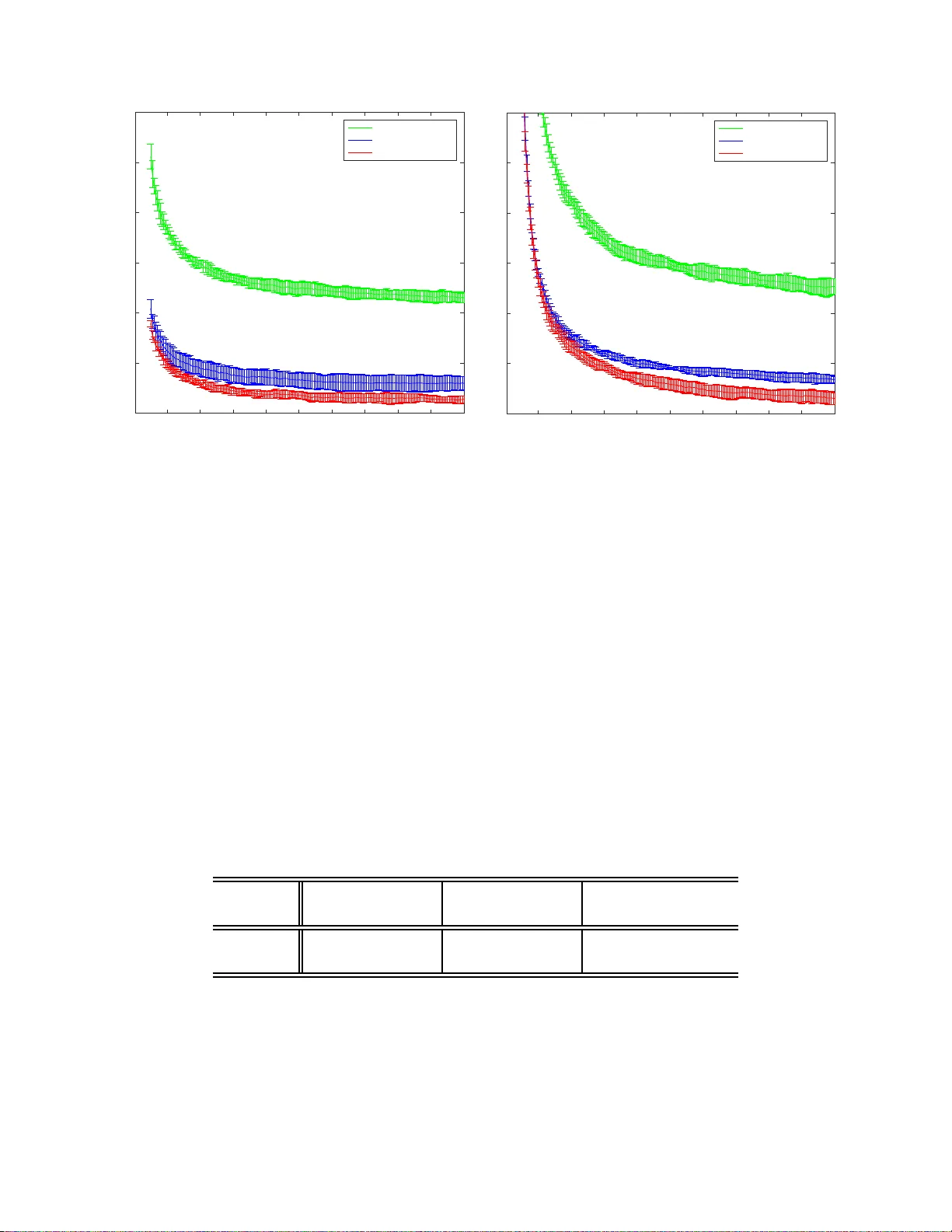
MA CHINE OLF A CTION USING TIME SCA TTERING OF SEN SOR MUL TIRESOLUTION GRA PHS LEONID GUGEL, YOEL SHKOLNISKY, AND SHAI DEKEL Abstract. In this pap er we construct a learning architecture for high dimensio nal time series sampled by sensor ar rangements. Using a redundant wav elet decomp osition o n a gra ph constructed ov er the sensor locations, o ur algo rithm is able to co nstruct discriminative features that exploit the m utual information betw een the sensors. The algor ithm then applies scattering netw orks to the time series gr aphs to create the feature spa ce. W e demonstr ate o ur metho d on a machine olfactio n problem, where one needs to classify the g as type a nd the lo cation wher e it o riginates from data sampled by an ar ray of sensors . Our exp erimental res ults clear ly demonstrate that our metho d outp e rforms classica l machine lea rning techniques used in pr evious studies. Contents 1. In tro duction 2 2. Olfaction datasets 3 3. Related studies on o dor classification 5 4. Mathematical bac kground 6 4.1. Redundan t w av elet decomp osition on g raph 6 4.2. Scattering con v olution netw ork on the g r a ph time series 8 4.3. Random F orest 11 5. Main algorithm 12 6. Results 14 6.1. F eature Space 14 6.2. Classification scenarios 14 6.3. Gas classification results 15 6.4. Detection of C O -concen tration 16 6.5. Source lo calizatio n 16 7. Conclusions 17 References 18 Date : F ebr uary 11, 2016 . Key wor ds and phr ases. sensor ar ray , electronic no se, metal-oxide s e nsors, o dor classification, o dor lo c ation, classification of high dimensio nal time series, scatter ing , deep lea rning, r andom forest. 1 2 1. Introduction Dev eloping c hemo-sensing solutions and standards for early w a rning ag ainst c hemical and bi- ological hazards ha s b een an activ e researc h area [3, 1 ]. T o construct an accurate and reliable c hemical w arning syste m, the information from sev eral sensors m ust b e in tegrated to pro vide a clear indication for the comp osition of the chemic al substances as w ell as their pro pagation profile. W e prop ose a machine learning approac h, that is based on recen t adv a nces, f o r classification and regression pro blems in mac hine olf action. Mac hine olfaction problems include o dor classification problems, gas consecration detection, and che mical source lo calization. Our algorithm consists t wo steps of feature generation and classification. T o transform the ra w data of the sensor array platform in to discriminativ e features, w e prop ose the Scattering Time Series on Graphs(STSG) transform, whic h is an hierarchic al feature extraction metho d from m ultiple time series. This transform is an extension of the recen tly prop o sed scattering transform for time series [26 , 13, 10, 12] and graph signals [15], to m ultiv a riate time series defined on a graph. The resulting features are then classified using a random forest (RF) based classifier [8, 9]. W e demonstrate and ev aluate our algo r it hm b y means of the Dataset from chem ical g as sensor arra y in turbulen t wind tunnel [17], av ailable through the UCI Mac hine L earning Rep ository [4]. This dataset has b een used to v alidate existing algorit hms [35, 34]. The structure o f our pa p er is as follows. In Section 2 w e describe a set of mac hine olf a ction problems w e wish to solv e and the dat aset that are used. In Section 3 w e review prio r art metho ds. In Section 4, w e presen t the theoretical building blo c ks of our metho d: a redundan t Haar w av elet decomp osition o v er a (p ossibly irregular) graph, the scattering conv o lution net work and Ra ndom F o rests. Equipped with these building blo cks , w e presen t in Section 5 the main contribution of this pap er, the STSG (Scattering of a Time Series on a Graphs) alg o rithm. Finally , in Section 6, w e show exp erimen t a l results of our metho dolo g y applied in the machine olfaction setting: o dor discrimination, o dor consecration, and o dor lo calization. W e compare the p erformance of our metho d with prior t ec hniques o f mac hine o lfaction [35, 34]. 3 Figure 1. Wind tunnel used to collect time series data from sensor array s[17]. 2. Olf action da t asets In this pap er w e use the dat a set “Ga s sensor arrays in op en sampling settings” from the UCI arc hiv e (Machine learning Rep ository) [4]. T his dat a set is a collection of multidimens ional time series da t a along with some static en vironmen ta l parameters that include the resp onses of a c hem- ical detection platform to differen t gases at different lev els of concen tratio n. The challenge is to dev elop mac hine learning tec hniques for gas classification a nd source prediction mo dels. In this section, w e review the dataset in details. The data in [4 ] w as collected in a 2 . 5 m × 1 . 2 m × 0 . 4 m wind tunnel test-b ed facilit y (see F igure 1), in t o whic h the gaseous substances of in terest w ere released. The wind tunnel op erates in a propulsion op en-cycle mo de, by contin uously drawing external turbulen t air t hroughout the tunnel and exhausting it bac k to the o utside, creating a relativ ely less turbulen t airflo w moving do wnstream tow a rds the end of the test field. In order to construct v a rious distinct artificial airflow s in the wind tunnel, the wind tunnel con tains a moto r - driv en exhaust fan at the outlet of the test section. The motor can b e set to rota t e at three differen t constan t sp eeds. The wind tunnel measures the am bien t temp erature a nd relat ive humid it y during the en tire exp erimen t. The c hemical detection platform inside the wind tunnel consists of b oar ds. Eac h b oard ha s eigh t commercialized metal- o xide gas sensors (MOX ) [2], whic h are sensitiv e to rapid c hanges in the analytes concen tra tion. Th us, the output of eac h b oard is an 8-dimensional time series. The c hemical detection platform consists of columns of nine b oards each lo cated at six equally-spaced p ositions along the wind tunnel, that is, a total of 72 sensors p er lo cation (see Figure 1). Figure 2 depicts a typic al time-series resp onse of one b oard. The sensor resp onses are affected b y the air turbulence in the wind t unnel and dep end on the concentration of the gas substance. As the op erating tempera t ure of the sensors affects their p erformance, it is a dj ustable b y setting the v olt a ge of the built-in heater of eac h sensor to one of fiv e differen t lev els. 4 Figure 2. Multiv ariate resp onse of a 8- sensor array when methane is released in the wind tunnel [17]. The dataset [4] w as generated b y releasing ten differen t types o f gas in to the wide t unnel: acetone, acetaldeh yde, ammonia, butanol (buty l-alcohol), ethy lene, methane, methanol, carb on mono xide, b enzene , to luene, a nd carb on mono xide(CO). Eac h kind of c hemical substance is released a t same nominal concen tratio n v alues at the outlet of the ga s source in parts-p er-million b y volume (ppm v).The CO w as released in t wo different nominal concen tratio ns. The v alue of concen tration at gas source is from 10 0 ppm to 400 ppm. Note that the actual concen tration in t he wind tunnel decreases as the generated g as plume spreads out along the tunnel. F o r eac h gas released, the motor of the exhaust fan w as set to one of three ro tation sp eeds. A turbulen t airflow was thereby g enerated within the wind tunnel. The outputs of the sensors a t eac h of the six lo cations in the wind tunnel w ere measured separately , resulting in six 7 2 -dimensional time series datasets capturing the che mical analyte circulated throughout the wind t unnel. The temp erature of all sensors remained fixed during the measureme n t. After eac h test, the wind tunnel was thoroughly v en tilated. The measuremen t w as rep eated for t hree differen t a ir v elo cities and fiv e o p erating temp eratur es. F or each combination of the t yp e of gas, airflow v elo cit y , and temp erature, the measuremen t (generation of time-series) w as rep eated 20 times. The time-series measure at eac h lo cation w a s sampled for approx imately 250 seconds, with 10 samples p er second, that is, a tota l of ab out 25 00 samples p er lo cation p er exp erimen t. The time series measured at all lo cations w as fully sync hronized, although each w as o f a sligh tly different length. The data f or eac h of the ten g a s classes was collected 20 times for each three sp eeds, five t emp era t ur es mo des and six lo cations. The r esulting data set th us consists of 18,000 72-dimensional time series. 5 In addition, each exp erimen t recorded the a m bient temp erature and relative humidit y during the experiment. Although these parameters are also represen ted as time series, they hav e v ery low v a riance and can th us b e represen t ed b y their a v erage v alues. F or a mo r e detailed description of the exp erimental proto col see [17, 35]. 3. Re la ted studies on odor class ifica t ion Sev eral previous studies [27, 28, 34, 35] ha v e considered the pr o blem of o dor classification. These studies all follow the same approac h of extracting features from t he data follow ed by some classification sc heme. Earlier approaches of o dor classification problems [27, 28] use f eatur es extracted by applying step wise discriminan t analysis (DA) t o the short-time F ourier transform ( STFT), follow ed by classification of these features with an L V Q (learning v ector quan tizat io n) neural netw ork. The F o urier p o w er sp ectrum of time series X ( t ) is defined by F w ,φ X ( t, ξ ) :=     Z X ( τ ) w ( t − τ ) e − iξ τ dτ     2 ∗ φ ( t ) , where w is a short-time low pass filter, φ ( t ) is a normalized smo othing windo w, and ξ is a f requency v a lue. The F ourier p o w er sp ectrum is defined as the exp ected v alue of square of the mo dulus of Short Time F ourier T ransform(STFT L 2 -momen ts) (3.1) ¯ F w ( ξ ) = E t [ F w ,φ X ( t, ξ )] . Then, the STFT-based feature mapping of time series X ( t ) is Φ : X → ¯ F ω ( ξ ) , ξ ∈ Ξ , where Ξ is a giv en set of f requencies . As t he STFT feature extraction method constitutes prior art f or o ur scattering approach , we applied it to our data as a p erformance b enc hmark. Recen t approac hes [3 5, 34] use more elab orate statistical mo deling of the data , as describ ed b elo w. Moreo v er, they hav e b een applied to the data set describ ed in Section 2 and are thu s of greater in terest to us. In this section we briefly describ e these alg orithms [35, 34], whic h are used in Section 6 as p erformance b enc hmarks. The study [34] mo dels the time series at the output o f the sensors, denoted b y X ( t ), using an auto-regressiv e linear mo del of order p [16, 24] X ( t ) = C + p X i =1 A i X ( t − i ) + e t where e t is a sto c hastic noise term, and C , A 1 , . . . , A p are parameters determined from the g iv en observ atio ns. 6 The parameters represe n t the time series C , A 1 , . . . , A p in the sense that the parameters can predict its v alue a t time t from past observ a tions, allowing for an error e t . Once these parameters ha v e b een estimated, we ma p eac h time series X ( t ) to its feature ve ctor b y ( C , A 1 , . . . , A p ) and use these v ectors as the input for the classification step. The classification step in [34] uses a k ernel SVM with a Gaussian kerne l function. The idea b ehind k ernel SVMs is to use a function k ( x, x ′ ) that measures the similarity b et w een the f eat ur es corresp o nding to eac h pair of instances in t he dataset. The most commonly used function is the Gaussian k ( x, x ′ ) = exp( − γ k x − x ′ k 2 ) , where γ h yp er-parameter, whic h is usually learned b y cross-v alidation. It can b e sho wn that the k ernel SVM algorithm is equiv alen t to mapping eac h f eat ur e v ector to some high (p ossibly infinite) dimensional space, follo w ed b y linear partitioning of tha t space. P a ssing the p oints through a k ernel function giv es rise to non- linear decision b oundaries, whic h cannot exist in linear classification. The results rep orted in [34] p ertain to a reduced dataset and simplified clarification/ prediction, whic h used only four ga ses and source lo cation only is classifie d to b e either the right or left sides of wind tunnel. The study [35] is of particular in terest to us since the conditions w ere exactly the same as in our study , namely classification of 10 gases with similar t r aining scenarios. The features space is the maximum of the normalized resp onse o f the sensors of each b oard. The classification sc heme of [35] is based on an inhibitory SVM classifier with a Gaussian k ernel, whose main concept is to train a classier f j for each p ossible lab el j = 1 , . . . , L where function f j constitutes the distance b et w een the correct lab el and the most offending incorrect answ er. F o r a more detailed description, see [20]. 4. Ma thema tical back groun d In this section w e presen t the theoretical background for our approa ch. In Section 4.1 w e presen t a generalization of the critically sampled Haa r w av elet tra nsform on gra phs [19] to an o v er-complete represen tation. This transform allows us to exploit correlations b etw een differen t sensing b oards and plays a critical role in our feature extraction pro cess. In Section 4.2, w e review the scattering con volution net w or k, in tro duced b y Mallat , whic h is one of building blo ck s of our metho d. Finally , in Section 4.3, w e provid e some details on the Random F orest algorithm. 4.1. R edundan t w a v elet decomp osition on graph. Let G = ( V , E ) b e an undirected and un weighed graph, where V = { v i } N i =1 is the v ertex set and E ⊂ V × V is the edge set. The m ultiscale folder-decomp osition [19] V = {V j } J j =0 is collection of v ertex set partitions where V 0 = V is at resolution zero and for j > 0 , V j = { υ j i } n j i =1 , n j = 2 − j N , with υ j i := υ j − 1 α i ∪ υ j − 1 β i . That is, the i -fo lder υ j i at lev el j is obtained by grouping t w o folders υ j − 1 α i and υ j − 1 β i from previous scale j − 1. A function X : G → R n on a graph G is defined b y mapping eac h v ertex v ∈ V to X ( v ) ∈ R n . The dot-pro duct of t w o functions X 1 , X 2 : G → R , is defined b y 7 (4.1) h X 1 , X 2 i G := X v ∈ G X 1 ( v ) · X 2 ( v ) . W e now define an Haar w av elet ortho-basis tra nsform o v er a folder decompo sition V . The Haar w av elet is a function on the graph G whic h is defined for eac h folder υ j i b y (4.2) ϕ j,i := 1 v j − 1 α i − 1 v j − 1 β i , where 1 W is the indicator function on the set W ⊂ V of the graph G , giv en by 1 W ( v ) = ( 1 if v ∈ W 0 otherwise According to [19], the set of functions { ϕ j,i } is an or t hogonal system defined o n the graph G = ( V , E ). The set (4.3) Φ V := { ϕ j,i ∪ 1 v j i } n j i =0 , such tha t n j = 2 − j N and 0 ≤ j ≤ J defines redundan t w av elets on the graph G. Note that on eac h lev el j , there are 2 − j N folders and that the maxim um scale of a folder- decomp o sition is K max = ⌊ log 2 N ⌋ . The application of the Haar tr a nsform to a signal X defined on a graph G pro ceeds as follow s. F or first scale k =1, the Haar co efficien ts are (4.4) ( X 1 ( i, 0) = h 1 v 1 i , X i G , X 1 ( i, 1) = h ϕ i, 1 , X i G . Then, for k = 2 , ..., K max , (4.5) ( X k ( i, 2 j ) = h 1 v k i , X k − 1 ( i, j ) i G , X k ( i, 2 j + 1) = h ϕ i,k , X k − 1 ( i, j ) i G . where i = 1 . . . 2 − k d. Observ e that when X ( t ), t ∈ T , is in fact a time series signal ov er the graph, then w e use the notation X k ( t, i, j ) for the time dep enden t m ultiscale Haar co efficien ts. Next, w e in tro duce a g eneralization of the redundan t wa v elet tra nsform [7, 31] to functions de- fined o n a gra ph. This approac h is effectiv e fo r signal pro cessing and pattern recognition problems suc h as imag e denoising [29] and sp eec h recognition [33]. Our approac h is to build a redundan t sc heme of w av elet decomp osition by o v erlapping the folders a t eac h lev el. Figure 3 illustrates a m ultiscale decomp osition with folder ov erlapping, whic h leads to a n ov er-complete wa v elet repre- sen tatio n of a signal o v er a graph domain. It is easy to demonstrate that the system of redundan t Haar-functions Φ V defined in ( 4 .3), where V is a folder decomp osition with o v erlapping, is not nec- essarily an ortho gonal basis. Ho w eve r, redundan t Haar functions pro vide more m utual informatio n b et w een v ertices. F o r our olfaction problem, an o v erlapp ed folder decomp osition using the neighborho o d relation- ships of the b oards. In Figure 4, we can see the Haar w a v elet lifting sc heme, where ov erlapping 8 Figure 3. Multiscale folder-decomp osition with ov erlapping. Figure 4. Multiscale folder-decomp osition with ov erlapping Bo a rd P o sition is applied on cen ter b oards of the line p o sition. Due t o the wind direction in the tunnel, the air wind tunnel generates a diffusion c hemical analyte. Therefore, cen tralized sensing b oards con t ain more informativ e time series data [35]. 4.2. Scatt ering con volution netw ork on the graph time series. In this section we r eview scattering con volution netw orks and their adaptations for a graph time series. In 4.2.1, w e review fundamen ta ls of con v olutional net w o r ks and deep learning. In 4.2.2 , w e r eview the w av elet-based scattering net w ork for time series. In 4.2.3, we emphasize the stabilit y prop erties of the w av elet approac h, whic h constitute an adv antage ov er the F ourier p o w er sp ectrum. In 4.2.4 , w e define feature extraction and classification metho ds based o n scattering. 4.2.1. F undamentals of Conv o lution Networks and De ep L e arning. Deep learning (DL) arc hit ec- tures [6 ] are neural net work-based a lg orithms mo deled to mimic the functionalit y of the human nerv ous system. The DL metho ds ha v e b een success fully a pplied in a v ariety of pattern recognition 9 problems suc h as computer vision (face recognition, image classification, and annota tion), natura l language pro cess ing, sp eec h recognition, and audio represen tations signals. Learning is achie v ed through hierarc hical feature extraction o f the observ ed data. The main idea is to apply nonlinear pro cessing on the data that flows b etw een the lay ers. In fact, hierarchic al features are fitted w eight parameters of neural net works (free par a meters of eac h unit), which are calculated as the results of one complex optimization pro cess. The conv olutional neural net work (CNN) [22] is one the most p opular deep learning arch itectures for pattern recognitions problems for grid-based signals suc h as t ime series, images, and videos, suc h as ImageNet [21]. The CNN consists of units that use ov erlapping pa tc hes o f input signals to apply neurons [23]. In other w ords, the CNN learns a hierarc hical net of con v olutio ns (filters) of signals. Mallat intro duced a mathematical class of deep con v o lution net w orks [26], whic h is called ‘Sc at- tering Convolution Networks’ . The scattering conv olution net works is unsup ervised CNN arc hitec- ture for grid-based signals that are obtained b y cascading wa v elet t r a nsforms and mo dulus p o oling op erators with the av erage of the amplitude o f iterated w av elet co efficien ts. The scattering-based feature extraction is translation in v ariant and Lipsc hitz con t inuous to deformations [13]. When trying to apply DL/ CNN tec hniques in problems suc h as ours, a difficult y arises since the geometric configuration of the sensors is not neces sarily regular, as in image pro cessing where the pixels are w ell aligned on a uniform grid. Th us, in this w ork, the concept o f the uniform grid is replaced b y a graph structure. 4.2.2. S c attering c onvolution network. In this work, the Scattering netw ork is applied separately to each time series of the type X ( t ) = X k ( t, i, j ) computed b y the graph analysis of Section 4.1. A scattering conv o lution netw ork is obtained based on a cascade of w a v elet conv o lution and mo dulus op erators with smo othing op erator (low-pass filter) [2 6 , 10 , 14 ]. Let ψ ( t ) b e a complex w a v elet, whose real and imaginary parts a r e orthogonal and hav e the same L 2 -norm, and R R ψ ( t ) dt = 0 with | ψ ( t ) | = O ((1 + t 2 ) − 1 ) with dy a dic dilat io ns: ψ j ( t ) = 2 − j ψ (2 − j t ) , ∀ j ∈ Z . The w av elet transform of time series X ( t ) at scale 2 j X ⋆ ψ j ( t ) = Z R X ( u ) ψ j ( t − u ) du. W e calculate the absolute v alue of the complex v alue co efficien t U 1 [ j ] X ( t ) = | X ⋆ ψ j ( u ) | . F o r eac h sequence of indices ¯ p = ( j 1 , . . . , j m ) : j 1 < j 2 < . . . j m the or der- m sc attering pr op agator U [ p ] is defined b y: U m [ ¯ p ] X ( t ) = U [ j m ] . . . U [ j 1 ] = || . . . || X ⋆ ψ j 1 | ⋆ ψ j 2 | . . . | ⋆ ψ j m ( t ) | 10 Figure 5. Tw o lev els scattering conv olution netw ork of time series X ( t ) with scat- tering propagators U [ j 1 ] a nd U [ j 1 , j 2 ] The windowe d sc attering S m,J [ ¯ p ] (scattering co efficien ts of order- m ) is defined by (4.1) S m,J [ ¯ p ] X ( t ) = U [ ¯ p ] X ⋆ φ J = || . . . || X ⋆ ψ j 1 | ⋆ ψ j 2 | . . . | ⋆ ψ j m ( t ) | ⋆ φ J where j 1 < . . . < j m < J a nd φ J ( t ) = 2 − J φ (2 − J t ) is low-pass filter with 2 J scale and R φ ( t ) dt = 1. The scattering op erator S J X ( t ) aggregates all scattering co efficien ts with order until lay er M (4.2) S J X ( t ) = ( S m,J X ( t )) 0 ≤ m ≤ M where S 0 ,J X ( t ) = X ⋆ φ J . The iterated pro cedure of scattering con v olution net w ork for a time series X ( t ) is illustrated in Figure 5. F o r most t yp es of the signals, suc h as audio, images, bio medical signals, a nd finance time series, it is sufficien t to compute the scattering co efficien t of lay ers 0,1 and 2 (M=2). S 2 ,J X =    S 0 ,J X S 1 ,J [ j 1 ] X S 2 ,J [ j 1 , j 2 ] X    j 1 ,j 2 ∈ Λ 4.2.3. S c attering Deformation stability. The efficiency of a scattering represen tation comes from its inv ariance to lo cal tra nslatio ns due to conv olutions with φ j and from its a bility to linearize deformations, that is, its stabilit y to time-w arping. The F ourier transform is unstable to deformation b ecause dilating a sin usoidal w a v e yields a new sinu soidal wa v e of different frequency that is orthogonal to the original one [32]. Let us define the deformation op erato r D τ of signal X ( t ) D τ X ( t ) = X ( t − τ ( t )) 11 where τ ( t ) non-constan t deformation t erm. As pro ven in [2 6, Theorem 2.12], the scattering t r ans- form S J of a signal X with compact supp ort is Lipsc hitz contin uous under action of deformation op erator D τ . (4.3) k S J ( D τ X ) − S J ( X ) k ≤ C M k X k  2 − J | τ | ∞ + | ∇ τ | ∞  where | τ | ∞ = sup t | τ ( t ) | and |∇ τ | ∞ = sup t |∇ τ ( t ) | < 1 . This prop ert y guarantees stability of signals X ( t ). It is clear that the deformation error is small if the scaling f actor J is 2 J ≫ | τ | ∞ and t he signal X ( t ) is smo oth in L 1 meaning. In other w o rds, the scattering metric satisfies inv ariance to lo cal transformat io ns and deformat ions. 4.2.4. S c attering moments. As noted in Section 4.2.3 a b o v e, the scattering net w ork is stable un- der small deformation. It can therefore b e used a s a n effectiv e feature space f or many kinds of classification and regression problems. State-of-the-a r t results o f the scattering approach hav e b een o btained fo r handwritten digit recognition and texture classification [11] compared to con v olution neural net works (CNN) [23, 30] and dictionary learning (DL) [25]. Scattering momen ts are defined as exp ected v alues ov er time of scattering co efficien ts, for each path ¯ p = ( j 1 , . . . , j m ) : j 1 < j 2 < . . . j m ¯ S [ ¯ p ] X = E ( S m,J [ ¯ p ] X ) = E ( U m [ ¯ p ] X ) F o r finite time series signal | X ( t ) | = N ¯ S [ ¯ p ] X = 1 N N X t =1 || X ⋆ ψ j 1 | ⋆ ψ j 2 | . . . | ⋆ ψ j m ( t ) | According to [5, 11], the standard wa y to build feature space based on scattering momen ts for finite time series signal | X | = N is (4.4) Φ : X → ¯ S [ j 1 ] X ¯ S [ j 1 , j 2 ] X ! j 1 ,j 2 ∈ Λ where a scaling set Λ = { ( j 1 , j 2 ) : 1 ≤ j 1 = 2 z 1 /Q 1 ≤ N and 1 ≤ j 2 = 2 z 2 /Q 2 ≤ j 1 z 1 , z 2 ∈ Z } defines a filter bank of scattering transform, suc h that are num b er wa v elets p er o cta ve of t he first and the second la y er. Scattering momen ts hav e b een used as features space[5 ] for time series classification problems: m usical genre classification (GITZAN) and phone segmen t classification. In these kinds of signals, the b est state-of- the-art results were o btained b y a n SVM classifier with Gaussian k ernel. 4.3. R andom F orest. Ra ndo m forest ( R F) [8] is a p opular ensem ble learning metho d fo r clas- sification a nd regression. A t training time, a dive rse set of decision trees is constructed using randomization tec hniques. Their output is then av eraged to ov ercome t he p ot en tial bias of eac h tree. In some implemen ta tions, the decision trees are pruned to reduce v a riance. RF easily allows 12 a par allel arc hitecture to b e implemen ted in applications for testing and tra ining scenarios. R F has b een implemen ted in many recen t a pplications for classification and regression problems [3 6]. In t he curren t study , w e found RF to b e an effectiv e classifier for our mac hine olfaction problem. Due to the fact t ha t the R F a pproac h is based on an ensem ble of decision trees, the feature set consists of v ariables from differen t domains, including catego r ical a nd con tinuous v a r ia bles. This allo ws us to add a set of static parameters, suc h as a ir flo w ve lo city and o p erating temp era t ure, to the feature space of time series. Let a set of vec tors X tr = { x 1 . . . x n : x i ∈ R d } b e a tr a ining set consisting of n samples, eac h a d -dimension feature v ector with asso ciated respo nse v alues Y tr = { y 1 , y 2 , . . . , y n } that can b e categorical v ariables in a classification problem or con tinuous v ariables in a regression problem. The training data can b e interpreted as samples gov erned b y an unkno wn distribution from X × Y . The goal of the R F classifier is to learn (approx imate) the oracle function F : X → Y , suc h that learned function ˆ f is the b est a ppro ximation of F with resp ect to an error metric (loss f unction). In the tr ee ba gging approac h, for each k = 1 . . . N , the algorithm randomly selects samples with replacemen t from the training set { X tr k , Y tr k } in order to build decision trees { T k } . The final prediction function ˆ f , is a n a v erage of the predictions of the decision tree { T k } , or b y weigh ted v ot ing of the ensem ble. 5. Main algorithm In this section, w e presen t the main algorithm dev elop ed in this pap er, in which all the elemen t s in t r o duced in the previous sections are brought together. The feature construction is p erformed using the Scattering Time Series on Graph (STSG) .The computed feature v ectors, alo ng with the resp onse v ariables, serv e as the training set for an RF algo rithm. The STSG algorithm com bines t he Haar scattering transform o n the gra ph and standard w a v elet- based scattering net describ ed previously . The Haar scattering netw o rk ar chitecture for the signal defined on graphs (not time series) w a s describ ed in [15]. The scattering ar chitecture is o bt a ined b y cascading m ultiscale Haar wa v elet transform defined o n an em b edded subset (f o lders construc- tion [19]), but without redundan t wa v elet decomp osition. X denotes a m ultiv ariat e time series defined on an un w eigh t ed graph domain G = ( V , E ), with dim( V ) = d and finite time domain T X : G × T → R . The scattering time series on graphs X ( n, t ) defined b y: (5.1) S J,ℓ,k [ p ℓ , ˆ j ] X = S J,ℓ [ p ℓ ] X k ( t, i, ˆ j ) . S J,ℓ [ p ℓ ] consists of t w o actions. The first of these tw o actions is the calculation o f k -lev els at redundan t Haar w a v elet co efficien ts (4 .5) with respect to the selected folder decompo sition V . The arc hitecture of f o lder decomp osition V can b e deriv ed fro m our understanding of the geometry of 13 the sensing pla t f orm. The second action is t he calculatio n o f ℓ -leve ls scattering co efficien ts of time series suc h that p ℓ = j 1 , . . . j l , are their scaling paths (4.1). The f eature space o f signal X ( n, t ) consists of STSG momen ts, that is, the expected v alue scattering time series on graphs transform S J,ℓ,k [ p ℓ , ˆ j ] o ver time. (5.2) Φ : X → ¯ S V = E t h S J,ℓ,k [ p ℓ , ˆ j ] X ( t, . ) i . Our mac hine learning task is as follows : Giv en a set of training signals X tr , Y tr , such that eac h instance is a time series defined on the same graph G , the learning algorithm m ust seek a prediction function f : X → Y . Equipped with o ur training set, we calculate STSG moments ¯ S V ( x i ), x i ∈ X tr (see 5.2). The second step is applying dimensionalit y reduction of the STSG moments to d principal comp onen t s Φ : x i → Φ d ( ¯ S V ( x i )) , ∀ x i ∈ X tr . The dimensionalit y reduction increases stabilit y . The scattering domain lies on a low dimensional manifold [11]. In some of the classification scenarios, w e hav e additional information a b out eac h instance x i , whic h it is added to the feature space. Since our learning algorit hm is based on an RF classifier, with trees constructed ov er bagging of the training set, each iteration k b egins with random sampling { X k , Y k } from the full training set, follow ed b y feature mapping, ¯ S V ( x i ), x i ∈ X k . Algorithm 1 T raining Random F orest of Scattering Graph Net 1: pro cedure TrainRF ( X tr , Y tr ) 2: for k ← 1 , T do # Lo op f or ensem ble trees 3: ( X k , Y k ) ← Bagging ( X tr , Y tr ) # B agging : Ran- dom sampling with replacemen t 4: ¯ S V ( x i ) ← STSG ( x i ) , x i ∈ X k # Computing STSG momen ts 5: (Φ d k , P d k ) ← P C d { ¯ S V ( x i ) , x i ∈ X k } ) # F eatures space : Dimensionalit y reduc- tion to d principal comp onen ts 6: f k ← T reeGrow (Φ d k , Y k ) # G ro wing a decision tr ee with feature bagging 7: F ← F + f k # Ensem ble tree building 8: end for 9: F ← 1 N F # F ina l classifier uniform normalization 10: return F # Output: Final tree ensem ble and learned PCA transform 11: end pro cedure 14 6. Re sul ts In t his section w e demonstrate the application of our approa ch to mac hine olfaction problems. In Section 6.1 , w e review the ra w feature space. In Section 6.2 w e define classification scenarios. Finally , in Sections 6.3, 6.4 and 6.5, we compare our results with prior-art scattering tec hniques and state-of-the-a r t mac hine olfa ction tec hniques describ ed in Section 3. 6.1. F eature Space. T o t he STSG features ( see Section 5), we add some of the pre-established conditioning para meters describ ed in Section 2 • He ater voltage V H ∈ { 4 . 0 V , 4 . 5 V , 5 . 0 V , 5 . 5 V , 6 V } , • Airflow velo city measured in rotat io n p er minu te: r mp ∈ { 15 00 , 3900 , 550 } , • Nominal c onc en tr ation measured in part s-p er-million b y v olume(ppmv ). The features of am bien t temp erature and r elat ive h umidity are not included since they ha v e v ery low v ariance. O ur exp erimen ts clearly sho w that adding these static features significan tly impro v es the p erformance of the prediction alg orithm. In addition, the lo cation of eac h time series is kno wn, namely , the p osition a nd b oard n umber with resp ect to the c hemical source. The lo cation of the sensing b oar d is (6.1) F loc = { X pos × X bord } , where • X pos ∈ { 0 . 25 , 0 . 5 , 0 . 98 , 1 . 18 , 1 . 40 , 1 . 4 5 } , • X board = 0 . 13 : 0 . 13 : 1 . 2. 6.2. Classification scenarios. Our results are for complex scenarios of gas classification and source detection. These scenarios are motiv ated by prop osals of the Departmen t o f Defense (DoD ) for the deve lopmen t of chemo-sen sing solutions and standards for early w arning and protection of military forces against p otential c hemical and biological attacks (see [1 ],[3]). Sp ecifically , the scenarios are as follows : • Ga s classification problem (10 lab els), • Ga s concen trat io n prediction for C O only (binary classification problem: 1 , 000 ppm and 4 , 00 ppm only), • Source lo calizatio n problem prediction of source lo cation with resp ect to lo cal co ordinat es in the wind tunnel. In all the ab o ve scenarios, w e applied learning with/without static features and with/without source lo cation information. Based on prior studies, w e constructed tw o w a ys to aggregate ra w features: (1) B o ard Column [35] agg regating all nine b oards fr o m than same p osition to a 72-dimension time series, (2) Single Board [34 ] using only the 8-dimension time series from a single b oard. 15 The ‘Single Board’ scenario is significan tly more difficult b ecause fewe r features are used. W e compared our results with frequency-domain features based on short-time F ourier transforma t io n (3.1) and simple features based first tw o statistical momen ts of eac h t ime series of sensor resp onse. In other w o rds, w e compared three groups of features: (1) STSG f eatur es (5.2 ) , (2) Sta t istical moments, (3) F ourier P o w er sp ectrum(STFT L 2 -momen ts) (3.1). F o r these three groups of features, we applied the same RF classifier with 2 0 0 grown trees. The error rate w as calculated as exp ected v alue and v ariance of 5-fo lder cross v alidation. 6.3. Gas classification results. T able 1 sho ws the classification p erformance of Board Column suitable for the conditions [35]. The p erformance of the random forest classifier for all three groups of features is significan tly b etter than the mean results of a previous study [35]. As sho wn, using our STSG features pro vides significan tely b etter p erformance in the more complex scenarios. T able 1. Classification p erformance of ‘Bo ar d Col umn ’ scenario .T esting error rate R F mo dels with prop osed STSG-algorithm, Short Time F o urier T rans- form(STFT) a nd statistical mo ments features, with/withput static features and with/withput lo cation information Static feature Lo cation STFT Statistical momen ts STSG [35] F ALSE F ALSE 2.52%( ± 0.09%) 0.574%( ± 0.07%) 0.47%( ± 0.07%) 7.89% TR UE 2.41%( ± 0.16%) 0.58%( ± 0.0 6 %) 0.48%( ± 0.03%) TR UE F ALSE 1.26%( ± 0.15%) 0.09%( ± 0.07%) 0.2 6%( ± 0.08%) TR UE 1.31%( ± 0.25%) 0.09%( ± 0.02%) 0.2 4%( ± 0.07%) A comparison in the ’Single Bo ar d’ scenario is presen ted in T able 2. T able 2. Class ification p erformance of ‘Single Bo ar d’ scenario . T esting error rate R F mo dels with STSG, STFT a nd statistic momen ts feat ures with/without static and lo cation information Static features Lo cation STFT Statistic momen ts STSG F ALSE F ALSE 19.68%( ± 0.37%) 24.9 6 %( ± 0.15%) 18.11%( ± 0.11%) TR UE 14.74%( ± 0.20%) 18.2 0 %( ± 0.11%) 13.63%( ± 00.20%) TR UE F ALSE 3.15%( ± 0.12%) 4.78%( ± 0.08%) 2.80%( ± 00.08%) TR UE 2.30%( ± 0.07%) 3.15%( ± 0.05%) 2.14%( ± 0.03%) Figure 6 shows error bars on learning curv es of v a lidation error and out-of- bag error ov er the n umber of grown classification trees in the random for est ensem ble fo r each kind of features. The STSG learning curv es hav e the fastest deca y rate. This prov es the learnabilit y of the prop osed metho d. 16 Number of grown trees 20 40 60 80 100 120 140 160 180 200 Validation error rate 0.02 0.025 0.03 0.035 0.04 0.045 0.05 Learning curves of validation error Statistic moments STFT STSG Number of grown trees 20 40 60 80 100 120 140 160 180 200 Out-of-bag error rate 0.02 0.025 0.03 0.035 0.04 0.045 0.05 Learning curves of out-of-bag error Statistic moments STFT STSG Figure 6. Learning curv es of the v alidat io n error and o ut-of-bag errors of classifi- cation p erformance of Single Boa rd scenario scenario. 6.4. Det ection of C O -concen tr ation. W e no w address a binar y classification problem, in which the goal is t o determine concen tra t io n of the C O substance (carb on mono xide). Note that the given dataset includes ev ery c hemical substance in the exp erimen t in only one nominal concen tration, except for the carb on monox ide, whic h w as collected in t w o differen t concen trations of 1 , 000 ppm and 4 , 000 ppm. W e built a subset with binary lab eling from a g iv en dataset that contained only exp eriments with C O . W e then applied our RF classifier for compared feature space. T able 3 presen ts the classification p erformance o f the Single Board scenario of the binary classification problem. Note that, in this scenario, w e cannot compare results with static features b ecause these features hav e b een sim ulat ed with differen t unique static parameters. T able 3. Classification p erformance of ’Single Bo ar d scenario for C O con- cen t ration . T esting error rate of R F classifier of prop osed STSG, STFT, a nd sta- tistical momen ts features space with/without lo cation information . Lo cation STFT Statistic momen ts STSG F ALSE 0.30%( ± 0.05%) 1.00%( ± 0.16 %) 0.24%( ± 0.07%) TR UE 0.26%( ± 0.06%) 0.61%( ± 0.10 %) 0.20%( ± 0.05%) The prop osed STSG feature space clearly demonstrates p erfo rmance that is sup erior to that of other metho ds.. W e did not apply this pro blem Board Column, b ecause Board Column scenario for all gases has p erfect p erformance yet. 6.5. Source lo calization. The source lo calization scenario is a learning of regression mo del for high a ccuracy detection of MO X-sensors lo cation with respect to the ga s substance. T ables 4 a nd 17 5 show the ra te error of the compared features space. The t w o types of features ag gregation, Board Column and Single Board scenarios, w ere used respective ly . The error rat e is the L 2 -norm error in meters b et w een sensor b oard lo cation and predicted lo cation. No te that if we use feature aggregation b y Single Board, the classifier predicts the 2D lo cation of t he sensing b o a rd F loc (6.1). When feature aggr ega tion by Bo a rd Column is used, the classifier predicts distance of line p osition only X pos . T able 4. Lo cation prediction p erformance of ’Bo ar d Col umn ’ : L 2 -norm error in meters with resp ect to source lo cation Static F eatur es STFT Statistic momen ts STSG F ALSE 0.0 2 155( ± 0.00063 ) 0.00745 ( ± 0.00028) 0.00477( ± 0.00060) TR UE 0.02025( ± 0.00 076) 0.00 773( ± 0.00032 ) 0.00481( ± 0.00043) T able 5. Lo cation prediction p er formance of ’Single Bo ar d scenarios : L 2 - Norm error in meters with resp ect to source lo catio n Static features STFT Statistic momen ts STSG F ALSE 0.174( ± 0.001) 0.288( ± 0.001) 0.162( ± 0.001) TR UE 0.161( ± 0.010) 0.280( ± 0.006) 0.150( ± 0.008) 7. Conclusions In the curren t study w e presen ted a no vel metho dology that can b e used for pattern recognition problems in whic h the signals are collected fro m a n arra y of p ossibly non-uniform ensem ble of sensors. W e defined a nov el scattering transform for m ultidimensional time series on the graph (STSG), whic h used redundan t w av elet g raph decomp osition. In this study , w e fo cused on mac hine olfaction problems in whic h the dataset w a s obtained fr o m a c hemical g as sensor array in a turbulen t wind tunnel. W e applied our metho dolog y to three mac hine learning problems: classification of 10 different gases at v a rious concen trations, detection of C O consecration, and ch emical substance lo calization. The next step of this research is to dev elop the prop osed metho d fo r ma chine olf action in cases in volving turbulen t gas mixtures [1 8]. Another in teresting r esearch direction would b e to add soft sup ervise d le arning to sc attering net . Recen t adv a nces in classical deep learning , such as CNN, hav e demonstrated high accuracy p erformance. These metho ds a re based on the learning o f con volutional filters. Ho w ev er, it m ust b e noted that deep learning arc hitecture t ypically requires a large training dataset and the learning pro cess is computationally inten siv e. Recall that the learning pro cess when using scattering net w orks is faster since we use pre-designed filters. One could then consider ‘soft’ learning v ariant of the scattering netw o rk, where standard w av elet filters are used as initial filters and then optimization is applied to o nly a f ew wa v elet para meters. 18 Reference s [1] Chemic al and biolo gic al sensors s t andar ds s t udy. , http ://ha ndle.d tic.mil/100.2/ADA458370 , Accessed: 2015- 04-08 . [2] Figar o usa, inc. , http: //www. figarosensor.com/ , Accessed: 2 015-0 4-08. [3] Niosh p o cket guide to chemic al hazar d. , h ttp:/ /www.c dc.gov/niosh/npg/ , Accessed: 201 5-04- 08. [4] Uci machine le arning r ep ository: Gas sensor arr ay s in op en sampling sett ings data set , http:/ /arch ive.ics.uci.edu/ml/datasets/Gas+sensor+arrays+in+open+sampling+settings , Accessed: 2013- 06-05 . [5] J o akim And ´ en and St´ ephane Malla t, D e ep sc attering sp e ctrum , (20 1 3). [6] Y o shua B engio, L e arning de ep ar chite ctu r es for ai , F ounda tions and trends R  in Machine Learning 2 (2009 ), no. 1, 1–1 27. [7] Gr e gory Beylkin, On the r epr esentation of op er ators in b ases of c omp actly supp orte d wavelets , SIAM Journal on Numerical Analysis 29 (19 92), no . 6 , 1716 –174 0 . [8] Leo B r eiman, R andom for ests , Machine learning 45 (2001), no. 1, 5–32 . [9] Leo Breiman, Jerome F r iedman, Charles J Stone, and Richard A O lshen, Classific ation and r e gr ession tr e es , (1984). [10] J Br una , E Mallat, S Bac r y , and JF Muzy , Multisc ale intermitten t pr o c ess analysis by sc attering , a rXiv pre pr int arXiv:131 1.410 4 . [11] Joan B runa and St´ ephane Malla t, Classific ation with sc attering op er ators , a rXiv preprint arXiv:10 1 1.302 3 (2010). [12] , Audio textu r e synthesis with sc attering moment s , arXiv preprint arXiv:1 311.04 07 (2013). [13] , Invariant sc att ering c onvolution net works , Pattern Analysis and Machine Intelligence, IEEE T ransa c - tions on 35 (2013 ), no. 8 , 1872–1 886. [14] Joan Bruna, Stephane Mallat, E mmanu el Bacr y , and J e an-F ranco is Muzy , Intermitten t pr o c ess analysis with sc attering moments , ar Xiv pr eprint arXiv:13 11.410 4 (201 3). [15] Xu Chen, Xiuyuan Cheng, and St´ ephane Mallat, Unsu p ervise d de ep haar sc attering on gr aphs , Adv ance s in Neural Information Pro cessing Systems, 20 14, pp. 1709– 1717. [16] Marco Cuturi and Arnaud Doucet, Autor e gr essive kernels for time series , ar Xiv preprint arXiv:1 101.06 73 (2011). [17] Jordi F ono llosa, Ir ene Ro dr ´ ıguez-Luj´ an, Marc o T r incavelli, a nd Ram´ on Huerta, Dataset fr om chemic al gas sensor arr ay in turbulent wind tunnel , Data in Brief 3 (2015), 169 –174. [18] Jordi F onollo sa, Ire ne Ro dr ´ ıguez-L uj´ an, Ma rco T rincavelli, Alexander V er gara, and Ram´ on Huerta, Chemic al discrimination in turbu lent gas mixt ur es with mox sensors valida te d by gas chr omato gr aphy-mass sp e ctr ometry , Sensors 14 (201 4), no. 10 , 19 336–1 9353 . [19] Matan Gavish, B o az Nadler , and Ronald R Coifman, Multisc ale wavelets on tr e es, gr aphs and high dimensional data: The ory and appli c ations t o semi sup ervise d le arning , P ro ceedings of the 27th In ternationa l Conference on Machine Learning (ICML-1 0), 2010, pp. 367– 374. [20] Ram´ on Huerta, Shank ar V embu, Jos´ e M Amig´ o, Thomas Nowotn y , and Charles Elk an, Inhibition in multiclass classific ation , Neura l co mputatio n 24 (2012), no. 9, 247 3–25 0 7. [21] Alex Krizhev s ky , Ilya Sutskev er, a nd Geoffre y E Hin ton, Imagenet classific ation with de ep c onvolutional neur al networks , Adv ances in neura l info r mation pro cessing systems, 201 2, pp. 1 097–1 105. [22] Y ann LeCun, L´ eon Bottou, Y o shua Bengio, and Patric k Haffner, Gr adient-b ase d le arning applie d to do cument r e c o gnition , P ro ceedings of the IEEE 86 (199 8), no. 11 , 22 78–23 24. 19 [23] Y ann LeCun, Ko ray Kavukcuoglu, and Cl´ ement F ara bet, Convolutional networks and applic ations in vision , Circuits and Systems (ISCAS), Pr o ceedings of 201 0 IEEE International Symp osium on, IEEE, 2010, pp. 253– 256. [24] Helm ut L¨ utk epo hl, New int r o duct ion to multiple time series analysis , Springer Science & Bus ine s s Media, 2 007. [25] Julien Maira l, F rancis Bach, a nd Jea n Ponce, T ask-driven dictionary le arning , Pattern Analysis and Machine Int elligence, IEE E T ra nsactions on 34 (2012 ), no. 4, 7 91–80 4. [26] Stephane Ma llat, Gr oup invariant sc attering , Communications on P ure a nd Applied Ma thematics 65 (2012), no. 10, 1331 –1398 . [27] N Nimsuk and T Nak amo to, Im pr ovement of c ap ability for classifying o dors in dynamic al ly changing c onc ent r a- tion u sing qcm sensor arr ay and short-time fourier tr ansform , Senso rs and Actuato r s B : Chemical 1 27 (20 07), no. 2, 491 –496. [28] , Stu dy on the o dor classific ation in dynamic al c onc entr ation r obust against humidity and temp er atur e changes , Sensors and Actuator s B: Chemical 134 (20 08), no. 1, 252– 2 57. [29] Idan Ram, Michael Ela d, and Isr ael Cohen, R e dundant wavelets on gr aphs and high dimensional data clouds , Signal Pro cess ing Letters , IEEE 19 (2012), no. 5, 291– 294. [30] M Ranzato, F u Jie Huang, Y-L Bour eau, a nd Y ann LeCun, Unsup ervise d le arning of invariant fe atu r e hier ar- chies with applic ations to obje ct r e c o gnition , Computer Vision and Pattern Rec o gnition, 2007. CVPR’07 . IEEE Conference on, IEEE , 20 07, pp. 1– 8. [31] Mark Shensa, The discr ete wavelet tr ansform: we dding the a tr ous and mal lat algorithms , Signal P ro cessing , IEEE T ransa ctions o n 40 (19 9 2), no. 10, 2464 – 2482 . [32] Ronen T almon, St´ ephane Mallat, Hitten Zav eri, a nd Ronald Co ifman, Manifold le arning for latent variable infer enc e in dynamic al systems , (2014). [33] Hamid Reza T o hidypo ur, Sey yed Ali Sey yedsalehi, Hossein Behbo o d, and Hossein Roshandel, A new r epr esen- tation for sp e e ch fr ame r e c o gnition b ase d on r e dun dant wavelet filter b anks , Sp eech Communication 54 (201 2), no. 2, 256 –271. [34] Shank a r V em bu, Alexander V erg a ra, Mehmet K Muezzinoglu, and Ramon Huerta, On t ime series fe atur es and kernels for machine olfactio n , Sensors and Actuators B: Che mica l 174 (2012), 535–5 46. [35] Alexander V er gara , Jordi F o nollosa, Jona s Mahiques, Marco T rincav elli, Nikolai Rulko v, and Ramon Huerta, On t he p erformanc e of gas sensor arr ays in op en sampling systems using inhibitory supp ort ve ctor machines , Sensors and Actuators B: Chemical 185 (20 13), 462– 4 77. [36] An ta nas V erik as, Adas Gelzinis, a nd Marija Bacausk iene, Mining data with r andom for ests: A survey and r esults of new tests , Pattern Reco gnition 44 (2011), no. 2, 330 –349. School of Ma thema tical Sciences, Tel A viv U niversity,Rama t A viv, 6997801 Tel A viv, Israel E-mail addr ess : leong @post. tau.ac.il School of Ma thema tical Sciences, Tel A viv U niversity,Rama t A viv, 6997801 Tel A viv, Israel E-mail addr ess : yoels h@post .tau.ac.il URL : https ://sit es.go ogle.com/site/yoelshkolnisky/ School of Ma thema tical Sciences, Tel A viv U niversity,Rama t A viv, 6997801 Tel A viv, Israel E-mail addr ess : shai. dekel@ ge.com URL : http: //www. shaid ekel.com/