DECOrrelated feature space partitioning for distributed sparse regression

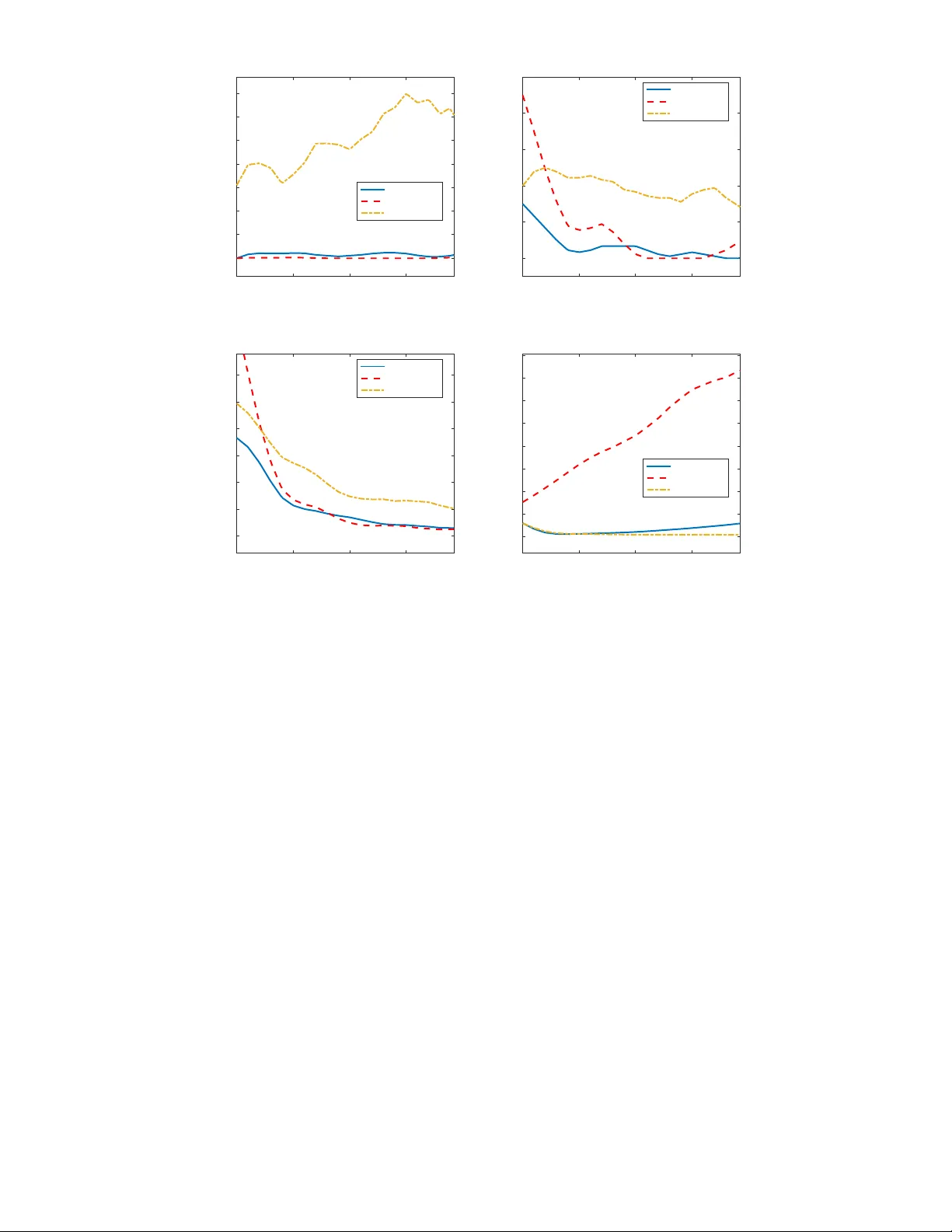
DECOrrelated feature space partitioning for distributed sparse regression Xiangyu W ang ∗ Da vid Dunson ∗ Chenlei Leng † F ebruary 15, 2016 Abstract Fitting statistical mo dels is computationally challenging when the sample size or the dimen- sion of the dataset is huge. An attractive approac h for down-scaling the problem size is to first partition the dataset in to subsets and then fit using distributed algorithms. The dataset can b e partitioned either horizontally (in the sample space) or vertically (in the feature space). While the ma jority of the literature fo cuses on sample space partitioning, feature space partitioning is more effective when p  n . Existing methods for partitioning features, how ev er, are either vulnerable to high correlations or inefficien t in reducing the mo del dimension. In this pap er, we solv e these problems through a new embarrassingly parallel framework named DECO for dis- tributed v ariable selection and parameter estimation. In DECO, v ariables are first partitioned and allocated to m distributed work ers. The decorrelated subset data within eac h w ork er are then fitted via any algorithm designed for high-dimensional problems. W e show that b y incor- p orating the decorrelation step, DECO can achiev e consistent v ariable selection and parameter estimation on each subset with (almost) no assumptions. In addition, the con vergence rate is nearly minimax optimal for b oth sparse and weakly sparse models and does NOT depend on the partition num ber m . Extensiv e numerical experiments are provided to illustrate the p erformance of the new framework. 1 In tro duction In modern science and technology applications, it has b ecome routine to collect complex datasets with a huge num b er p of v ariables and/or enormous sample size n . Most of the emphasis in the ∗ Departmen t of Statistical Science, Duk e Universit y , USA. † Departmen t of Statistics, Universit y of W arwic k, UK. 1 literature has b een on addressing large n problems, with a common strategy relying on partitioning data samples into subsets and fitting a mo del con taining all the v ariables to each subset (Mcdonald et al., 2009; Zhang et al., 2012; W ang and Dunson, 2013; Scott et al., 2013; W ang et al., 2015a, 2014; Minsker et al., 2015). In scientific applications, it is muc h more common to hav e huge p small n data sets. In such cases, a sensible strategy is to break the features into groups, fit a mo del separately to each group, and com bine the results. W e refer to this strategy as feature space partitioning, and to the large n strategy as sample space partitioning. There are sev eral recent attempts on parallel v ariable selection b y partitioning the feature space. Song and Liang (2014) proposed a Bay esian split-and-merge (SAM) approach in which v ariables are first partitioned in to subsets and then screened o ver eac h subset. A v ariable selection pro cedure is then performed on the v ariables that surviv e for selecting the final mo del. One cav eat for this approac h is that the algorithm cannot guarantee the efficiency of screening, i.e., the screening step tak en on eac h subset might select a large n umber of unimportant but correlated v ariables (Song and Liang, 2014), so the split-and-merge procedure could b e ineffectiv e in reducing the model dimension. Inspired by a group test, Zhou et al. (2014) prop osed a parallel feature selection algorithm b y rep eatedly fitting partial mo dels on a set of re-sampled features, and then aggregating the residuals to form scores for each feature. This approac h is generic and efficient, but the p erformance relies on a strong condition that is almost equiv alen t to an indep endence assumption on the design. In tuitiv ely , feature space partitioning is muc h more challenging than sample space partitioning, mainly b ecause of the correlations b etw een features. A partition of the feature space would succeed only when the features across the partitioned subsets w ere mutually independent. Otherwise, it is highly likely that any mo del p osed on the subsets is mis-sp ecified and the results are biased regardless of the sample size. In reality , how ever, mutually indep endent groups of features may not exist; Ev en if they do, finding these groups is lik ely more c hallenging than fitting a high-dimensional mo del. Therefore, although conceptually attractive, feature space partitioning is extremely c hal- lenging. On the other hand, feature space partitioning is straightforw ard if the features are indep enden t. Motiv ated b y this key fact, we prop ose a no v el em barrassingly-parallel framework named DECO b y de c orr elating the features b efore partitioning. With the aid of decorrelation, each subset of data after feature partitioning can now pro duce consisten t estimates even though the mo del on eac h subset is intrinsically mis-sp ecified due to missing features. T o the b est of our kno wledge, DECO is the first em barrassingly parallel framew ork sp ecifically designed to accommo date arbitrary 2 correlation structure in the features. W e show, quite surprisingly , that the DECO estimate, b y lev eraging the estimates from subsets, achiev es the same conv ergence rate in ` 2 norm and ` ∞ norm as the estimate obtained by using the full dataset, and that the rate do es not dep end on the n um b er of partitions. In view of the huge computational gain and the easy implementation, DECO is extremely attractiv e for fitting large- p data. The most related work to DECO is Jia and Rohe (2012), where a similar procedure w as intro- duced to improv e lasso . Our w ork differs substan tially in v arious aspects. First, our motiv ation is to develop a parallel computing framework for fitting large- p data by splitting features, whic h can p oten tially accommodate an y penalized regression metho ds, while Jia and Rohe (2012) aim solely at complying with the irrepresentable condition for lasso . Second, the conditions p osed on the feature matrix are more flexible in DECO, and our theory , applicable for not only sparse signals but also those in l r balls, can b e readily applied to the preconditioned lasso in Jia and Rohe (2012). The rest of the pap er is organized as follo ws. In Section 2, we detail the prop osed framework. Section 3 pro vides the theory of DECO. In particular, w e show that DECO is consistent for b oth sparse and w eakly sparse models. Section 4 presen ts extensiv e sim ulation studies to illustrate the p erformance of our framework. In Section 5, we outline future c hallenges and future w ork. All the tec hnical details are relegated to the App endix. 2 Motiv ation and the DECO framew ork Consider the linear regression model Y = X β + ε, (1) where X is an n × p feature (design) matrix, ε consists of n i.i.d random errors and Y is the resp onse v ector. A large class of approac hes estimate β b y solving the following optimization problem ˆ β = ar g min β 1 n k Y − X β k 2 2 + 2 λ n ρ ( β ) , where k · k 2 is the ` 2 norm and ρ ( β ) is a p enalty function. In this pap er, we specialize our discussion to the ` 1 p enalt y where ρ ( β ) = P p j =1 | β j | (Tibshirani, 1996) to highlight the main message of the pap er. As discussed in the introduction, a naiv e partition of the feature space will usually giv e un- satisfactory results under a parallel computing framew ork. That is why a decorrelation step is 3 in tro duced. F or data with p ≤ n , the most intuitiv e w a y is to orthogonalize features via the singu- lar v alue decomp osition (SVD) of the design matrix as X = U D V T , where U is an n × p matrix, D is an p × p diagonal matrix and V an p × p orthogonal matrix. If w e pre-multiply b oth sides of (1) by √ pD − 1 U T , we get √ pD − 1 U T Y = √ pV T β + √ pD − 1 U T ε. (2) It is obvious that the new features (the columns of √ pV T ) are mutually orthogonal. An alternative approac h to a void doing SVD is to replace √ pD − 1 U T b y √ pU D − 1 U T = ( X X T /p ) + 2 , where A + denotes the Moore-Penrose pseudo-inv erse. Thus, w e hav e ( X X T /p ) + 2 Y = √ pU V T β + ( X X T /p ) + 2 ε, (3) where the new features (the columns of √ pU V T ) are m utually orthogonal. Define the new data as ( ˜ Y , ˜ X ). The mutually orthogonal prop erty allows us to decompose ˜ X column-wisely to m subsets ˜ X ( i ) , i = 1 , 2 , · · · , m , and still retain consistency if one fits a linear regression on eac h subset. T o see this, notice that each sub-model now tak es a form of ˜ Y = ˜ X ( i ) β ( i ) + ˜ W ( i ) where W ( i ) = ˜ X ( − i ) β ( − i ) + ˜ ε and X ( − i ) stands for v ariables not included in the i th subset. If, for example, w e would like to compute the ordinary least squares estimates, it follows ˆ β ( i ) = ( ˜ X ( i ) T ˜ X ( i ) ) − 1 ˜ X ( i ) ˜ Y = β ( i ) + ( ˜ X ( i ) T ˜ X ( i ) ) − 1 ˜ X ( i ) ˜ W ( i ) = β ( i ) + ( ˜ X ( i ) T ˜ X ( i ) ) − 1 ˜ X ( i ) ˜ ε where we retrieve a consistent estimator that con v erges in rate as if the full dataset were used. When p is larger than n , the new features are no longer exactly orthogonal to each other due to the high dimension. Nev ertheless, the correlations b et w een different columns are roughly of the order q log p n for random designs, making the new features approximately orthogonal when log( p )  n . This allows us to follo w the same strategy of partitioning the feature space as in the lo w dimensional case. It is worth noting that when p > n , the SVD decomp osition on X induces a differen t form on the three matrices, i.e., U is no w an n × n orthogonal matrix, D is an n × n diagonal matrix, V is an n × p matrix, and  X X T p  + 2 b ecomes  X X T p  − 1 2 . In this pap er, w e primarily fo cus on datasets where p is so large that a single computer is only 4 able to store and perform op erations on an n × q matrix ( n < q < p ) but not on an n × p matrix. Because the tw o decorrelation matrices yield almost the same prop erties, we will only presen t the algorithm and the theoretical analysis for ( X X T /p ) − 1 / 2 . The concrete DECO framework consists of tw o main steps. Assume X has b een partitioned column-wisely into m subsets X ( i ) , i = 1 , 2 , · · · , m (each with a maxim um of q columns) and distributed onto m mac hines with Y . In the first stage, we obtain the decorrelation matrix ( X X T /p ) − 1 / 2 or √ pD − 1 U T b y computing X X T in a distributed wa y as X X T = P m i =1 X ( i ) X ( i ) T and p erform the SVD decomp osition on X X T on a cen tral mac hine. In the second stage, each w ork er receiv es the decorrelation matrix, m ultiplies it to the local data ( Y , X ( i ) ) to obtain ( ˜ Y , ˜ X ( i ) ), and fits a penalized regression. When the model is assumed to b e exactly sparse, w e can potentially apply a refinemen t step b y re-estimating co efficien ts on all the selected v ariables simultaneously on the master mac hine via ridge regression. The details are provided in Algorithm 1. Algorithm 1 The DECO fr amework Initialization: 1: Input ( Y , X ) , p, n, m, λ n . Standardize X and Y to x and y with mean zero; 2: P artition (arbitrarily) ( y , x ) in to m disjoin t subsets ( y , x ( i ) ) and distribute to m mac hines; Stage 1 : Decorrelation 3: F = 0 initialized on the master machine; 4: for i = 1 to m do 5: F = F + x ( i ) x ( i ) T ; 6: ¯ F = √ p  F + r 1 I p  − 1 / 2 on the master machine and then pass back; 7: for i = 1 to m do 8: ˜ y = ¯ F y and ˜ x ( i ) = ¯ F x ( i ) ; Stage 2 : Estimation 9: for i = 1 to m do 10: ˆ β ( i ) = ar g min β 1 n k ˜ y − ˜ x ( i ) β k 2 2 + 2 λ n ρ ( β ); 11: ˆ β = ( ˆ β (1) , ˆ β (2) , · · · , ˆ β ( m ) ) on the master mac hine; 12: ˆ β 0 = mean ( Y ) − mean ( X ) T ˆ β for intercept. Stage 3 : Refinemen t (optional) 13: if # { ˆ β 6 = 0 } ≥ n then 14: # S parsification is needed before ridge regression. 15: M = { k : | ˆ β k | 6 = 0 } ; 16: ˆ β M = ar g min β 1 n k ˜ y − ˜ x M β k 2 2 + 2 λ n ρ ( β ); 17: M = { k : | ˆ β k | 6 = 0 } ; 18: ˆ β M = ( X T M X M + r 2 I |M| ) − 1 X T M Y ; return ˆ β ; Line 13 - 16 in Algorithm 1 are added only for the data analysis in Section 5.3, in whic h p is so massiv e that log( p ) w ould be comparable to n . F or suc h extreme cases, the algorithm ma y not scale do wn the size of p sufficien tly for ev en obtaining a ridge regression estimator afterw ards. Th us, a further sparsification step is recommended. This differs fundamentally from the merging step in 5 SAM (Song and Liang, 2014) in that DECO needs this step only for extreme cases where log( p ) ∼ n , while SAM alwa ys requires a merging step regardless of the relationship b etw een n and p . The condition in Line 16 is barely triggered in our exp eriments (only in Section 5.3), but is crucial for impro ving the p erformance for extreme cases. In Line 6, the algorithm in v erts X X T + r 1 I instead of X X T for robustness, because the rank of X X T after standardization will b e n − 1. Using ridge refinemen t instead of ordinary least squares is also for robustness. The precise choice of r 1 and r 2 will b e discussed in the numerical section. P enalized regression fitted using regularization path usually inv olves a computational complexity of O ( k np + k d 2 ), where k is the num b er of path segmen tations and d is the num b er of features selected. Although the segmentation n um b er k could b e as bad as (3 p + 1) / 2 in the worst case (Mairal and Y u, 2012), real data experience suggests that k is on a v erage O ( n ) (Rosset and Zhu, 2007), thus the complexity for DECO takes a form of O  n 3 + n 2 p m + m  in contrast to the full lasso whic h takes a form of O ( n 2 p ). As n is assumed to b e small, using DECO can substantially reduce the computational cost if m is prop erly c hosen. 3 Theory In this section, w e provide theoretical justification for DECO on random feature matrices. W e sp ecialize our atten tion to lasso due to page limits and will pro vide the theory on general p enalties in the long version. Because the tw o decorrelation matrices yield similar consistency prop erties, the theory will be stated only for ( X X T /p ) − 1 2 . This section consists of t w o parts. The first part pro vides preliminary results for lasso , when strong conditions on the feature matrix are imp osed. In the second part, we adapt these results to DECO and sho w that the decorrelated data will automatically satisfy the conditions on the feature matrix ev en when the original features are highly correlated. 3.1 Deterministic results for lasso with conditions on the feature matrix Define Q = { 1 , 2 , · · · , p } and let A c b e Q \ A for any set A ⊆ Q . The following theorem pro- vides deterministic conditions for lasso on sup-norm con v ergence, ` 2 -norm conv ergence and sign consistency . 6 Theorem 1. Under mo del (1) , denote the solution to the lasso pr oblem as ˆ β = ar g min β ∈R p 1 n   Y − X β   2 2 + 2 λ n k β k 1 . Define W = Y − X β ∗ , wher e β ∗ is the true value of β . F or any arbitr ary subset J ⊆ Q ( J c ould b e ∅ ), if X satisfies that 1. M 1 ≤ | x T i x i /n | ≤ M 2 , for some 0 < M 1 < M 2 and al l i , 2. max i 6 = j | x T i x j /n | ≤ min  1 γ 1 s , γ 2 λ q n  , for γ 1 > 32 M 1 , γ 2 ≥ 0 , q ≥ 0 and s = | J | , 3. k 1 n X T W k ∞ ≤ λ n / 2 , then any solution to the lasso pr oblem satisfies that k ˆ β − β ∗ k ∞ ≤ 3 M 1 γ 1 + 51 2 M 1 ( M 1 γ 1 − 7) λ n + 4 M 1 γ 1 γ 2 + 36 γ 2 M 1 ( M 1 γ 1 − 7) k β ∗ J c k 1 λ q n + 8 √ 3 γ 2 M 1 √ M 1 γ 1 − 7 k β ∗ J c k 1 2 1 λ 1+ q 2 n , wher e β ∗ J c is the sub-ve ctor of β ∗ c onsisting of c o or dinates in J c and k ˆ β − β ∗ k 2 2 ≤ 18 γ 2 1 sλ 2 n ( M 1 γ 1 − 32) 2 + 6 λ n k β ∗ J c k 1 + 32 γ 2 λ q n k β ∗ J c k 2 1 . F urthermor e, if β ∗ J c = 0 and min k ∈ J | β ∗ k | ≥ 2 M 1 λ n , then the solution is unique and sign c onsistent, that is, sig n ( ˆ β k ) = sig n ( β ∗ k ) , ∀ k ∈ J and ˆ β k = 0 , ∀ k ∈ J c . Theorem 1 partly extends the results in Bic k el et al. (2009) and Lounici (2008). The proof is pro vided in App endix A. Theorem 1 can lead to some useful results. In particular, we in vestigate t w o t yp es of mo dels when β ∗ is either exactly sparse or in an l r -ball defined as B ( r, R ) = { v ∈ R p : P p k =1 | v k | r ≤ R } . F or the exactly sparse mo del, w e ha v e the follo wing result. Corollary 1 (s-sparse) . Assume that β ∗ ∈ R p is an s-sp arse ve ctor with J c ontaining al l non-zer o indic es. If Condition 1 and 3 in The or em 1 hold and max i 6 = j | x T i x j /n | ≤ 1 γ 1 s for some γ 1 > 32 / M 1 , then we have k ˆ β − β ∗ k ∞ ≤ 3 M 1 γ 1 + 51 2 M 1 ( M 1 γ 1 − 7) λ n , k ˆ β − β ∗ k 2 2 ≤ 18 γ 2 1 sλ 2 n ( M 1 γ 1 − 32) 2 . 7 F urther, if min k ∈ J | β k | ≥ 2 M 1 λ n , then ˆ β is sign c onsistent. The sup-norm conv ergence in Corollary 1 resembles the results in Lounici (2008). F or the l r -ball w e hav e Corollary 2 ( l r − ball) . Assume β ∗ ∈ B ( r, R ) . If c ondition 1 and 3 in The or em 1 hold and max i 6 = j | x T i x j /n | ≤ λ r n γ 1 R for some γ 1 > 32 / M 1 , then we have k ˆ β − β ∗ k ∞ ≤  3 M 1 γ 1 + 51 2 M 1 ( M 1 γ 1 − 7) + 4 M 1 γ 1 + 36 M 1 ( M 1 γ 1 − 7) + 8 √ 3 M 1 √ M 1 γ 1 − 7  λ n , k ˆ β − β ∗ k 2 2 ≤  18 γ 2 1 ( M 1 γ 1 − 32) 2 + 38  Rλ 2 − r n . 3.2 Results for DECO without conditions on the feature matrix In this part, we apply the previous results from the lasso to DECO, but without the restrictive conditions on the feature matrix. In particular, w e prov e the consistency results for the estimator obtained after Stage 2 of DECO, while the consistency of Stage 3 will then follow immediately . Recall that DECO w orks with the decorrelated data ˜ X and ˜ Y , which are distributed on m dif- feren t machines. Therefore, it suffices for us to verify the conditions needed b y lasso for all pairs ( ˜ Y , ˜ X ( i ) ) , i = 1 , 2 , · · · , m . F or simplicit y , w e assume that ε follows a sub-Gaussian distribution and X ∼ N (0 , Σ) throughout this section, although the theory can b e easily extended to the situation where X follows an elliptical distribution and ε is heavy-tailed. As describ ed in the last section, DECO fits the follo wing linear regression on each work er ˜ Y = ˜ X ( i ) β ( i ) + ˜ W ( i ) , and ˜ W ( i ) = ˜ X ( − i ) β ( − i ) + ˜ ε, where X ( − i ) stands for v ariables not included in the i th subset. T o v erify Condition 1 and Condition 2 in Theorem 1, we cite a result from W ang et al. (2015b) (Lemma 7 in App endix C) which prov es the boundedness of M 1 and M 2 and that max i 6 = j | ˜ x T i ˜ x T j | /n is small. V erifying Condition 3 is the k ey to the whole proof. Different from the conv en tional setting, ˜ W now con tains non-zero signals that are not indep endent from the predictors. This requires us to accurately capture the b ehavior of the follo wing tw o terms max k ∈ Q   1 n ˜ x T k ˜ X ( − k ) β ( − k ) ∗   and max k ∈ Q   1 n ˜ x T k ˜ ε   , for whic h we ha v e Lemma 1. Assume that ε is a sub-Gaussian variable with a ψ 2 norm of σ and X ∼ N (0 , Σ) . 8 Define σ 2 0 = v ar ( Y ) . If p > c 0 n for some c 0 > 1 , then we have for any t > 0 P  max k ∈ Q 1 n | ˜ x T k ˜ ε | > σ t √ n  ≤ 2 p exp  − c ∗ c 2 0 2 c ∗ c 2 (1 − c 0 ) 2 t 2  + 4 pe − C n , P  max k ∈ Q 1 n   ˜ x T k ˜ X ( − k ) β ( − k ) ∗   ≥ √ σ 0 − σ t √ n  ≤ 2 p exp  − c 3 ∗ 2 c 2 4 c ∗ 2 t 2  + 5 pe − C n , wher e C , c 1 , c 2 , c 4 , c ∗ , c ∗ ar e define d in L emma 7. W e now provide the main results of the pap er. Theorem 2 (s-sparse) . Assume that β ∗ is an s-sp arse ve ctor. Define σ 2 0 = v ar ( Y ) . F or any A > 0 we cho ose λ n = Aσ 0 q log p n . Now if p > c 0 n for some c 0 > 1 and 64 C 2 0 A 2 s 2 log p n ≤ 1 , then with pr ob ability at le ast 1 − 8 p 1 − C 1 A 2 − 18 pe − C n we have k ˆ β − β ∗ k ∞ ≤ 5 C 0 Aσ 0 8 r log p n , k ˆ β − β ∗ k 2 2 ≤ 9 C 0 A 2 σ 2 0 8 s log p n , wher e C 0 = 8 c ∗ c 1 c ∗ and C 1 = min { c ∗ c 2 0 8 c ∗ c 2 (1 − c 0 ) 2 , c 3 ∗ 8 c 2 4 c ∗ 2 } ar e two c onstants and c 1 , c 2 , c 4 , c ∗ , c ∗ , C ar e define d in L emma 7. F urthermor e, if we have min β k 6 =0 | β k | ≥ C 0 Aσ 0 4 r log p n , then ˆ β is sign c onsistent. Theorem 2 lo oks a bit surprising since the conv ergence rate do es not dep end on m . This is mainly b ecause the b ounds used to v erify the three conditions in Theorem 1 hold uniformly on all subsets of v ariables. F or subsets where no true signals are allo cated, lasso will estimate all co efficien ts to be zero under suitable c hoice of λ n , so that the loss on these subsets will b e exactly zero. Thus, when summing ov er all subsets, w e retrieve the s log p n rate. In addition, it is worth noting that Theorem 2 guarantees the ` ∞ con v ergence and sign consistency for lasso without assuming the irrepresentable condition (Zhao and Y u, 2006). A similar but w eak er result w as obtained in Jia and Rohe (2012). Theorem 3 ( l r -ball) . Assume that β ∗ ∈ B ( r, R ) and al l c onditions in The or em 2 exc ept that 64 C 2 0 A 2 s 2 log p n ≤ 1 ar e now r eplac e d by 64 C 2 0 A 2 R 2  log p n  1 − r ≤ 1 . Then with pr ob ability at le ast 9 1 − 8 p 1 − C 1 A 2 − 18 pe − C n , we have k ˆ β − β ∗ k ∞ ≤ 3 C 0 Aσ 0 2 r log p n , k ˆ β − β ∗ k 2 2 ≤  9 C 0 8 + 38  ( Aσ 0 ) 2 − r R  log p n  1 − r 2 . Note that σ 2 0 = v ar ( Y ) instead of σ app ears in the conv ergence rate in b oth Theorem 2 and 3, which is inevitable due to the nonzero signals contained in ˜ W . Compared to the estimation risk using full data, the results in Theorem 2 and 3 are similar up to a factor of σ 2 /σ 2 0 = 1 − ˆ R 2 , where ˆ R 2 is the co efficient of determination. Th us, for a mo del with an ˆ R 2 = 0 . 8, the risk of DECO is upper b ounded b y fiv e times the risk of the full data inference. The rates in Theorem 2 and 3 are nearly minimax-optimal (Y e and Zhang, 2010; Raskutti et al., 2009), but the sample requiremen t n  s 2 is slightly off the optimal. This requiremen t is ro oted in the ` ∞ -con v ergence and sign consistency and is almost unimpro v able for random designs. W e will detail this argument in the long version of the paper. 4 Exp erimen ts In this section, w e presen t the empirical performance of DECO via extensive numerical exp eriments. In particular, we compare DECO after 2 stage fitting ( DECO-2 ) and DECO after 3 stage fitting ( DECO-3 ) with the full data lasso ( lasso-full ), the full data lasso with ridge refinemen t ( lasso- refine ) and lasso with a naive feature partition without decorrelation ( lasso-naive ). This section consists of three parts. In the first part, we run DECO-2 on some sim ulated data and monitor its p erformance on one randomly chosen subset that contains part of the true signals. In the second part, we verify our claim in Theorem 2 and 3 that the accuracy of DECO do es not dep end on the subset num ber. In the last part, w e pro vide a comprehensiv e ev aluation of DECO’s p erformance b y comparing DECO with other metho ds under v arious correlation structures. The syn thetic datasets are from mo del (1) with X ∼ N (0 , Σ) and ε ∼ N (0 , σ 2 ). The v ariance σ 2 is chosen such that ˆ R 2 = v ar ( X β ) /v ar ( Y ) = 0 . 9. F or ev aluation purp oses, we consider fiv e differen t structures of Σ as b elow. Mo del (i) Indep endent pr e dictors . The supp ort of β is S = { 1 , 2 , 3 , 4 , 5 } . W e generate X i from a standard m ultiv ariate normal distribution with indep enden t components. The co efficients 10 are sp ecified as β i =      ( − 1) B er (0 . 5)  | N (0 , 1) | + 5 q log p n  i ∈ S 0 i 6∈ S. Mo del (ii) Comp ound symmetry . All predictors are equally correlated with correlation ρ = 0 . 6. The co efficients are the same as those in Model (i). Mo del (iii) Gr oup structur e . This example is Example 4 in Zou and Hastie (2005), for which w e allo cate the 15 true v ariables into three groups. Sp ecifically , the predictors are generated as x 1+3 m = z 1 + N (0 , 0 . 01), x 2+3 m = z 2 + N (0 , 0 . 01) and x 3+3 m = z 3 + N (0 , 0 . 01), where m = 0 , 1 , 2 , 3 , 4 and z i ∼ N (0 , 1) are independent. The coefficients are set as β i = 3 , i = 1 , 2 , · · · , 15; β i = 0 , i = 16 , · · · , p . Mo del (iv) F actor mo dels . This mo del is considered in Meinshausen and B ¨ uhlmann (2010). Let φ j , j = 1 , 2 , · · · , k b e independent standard normal v ariables. W e set predictors as x i = P k j =1 φ j f ij + η i , where f ij and η i are indep endent standard normal random v ariables. The num b er of factors is c hosen as k = 5 in the simulation while the co efficients are sp ecified the same as in Mo del (i). Mo del (v) ` 1 -b al l . This mo del takes the same correlation structure as Model (ii), with the co efficien ts drawn from Diric hlet distribution β ∼ D ir  1 p , 1 p , · · · , 1 p  × 10. This mo del is to test the p erformance under a weakly sparse assumption on β , since β is non-sparse satisfying k β k 1 = 10. Throughout this section, the performance of all the metho ds is ev aluated in terms of four metrics: the num ber of false p ositiv es ( # FPs ), the num b er of false negatives ( # FNs ), the mean squared error k ˆ β − β ∗ k 2 2 ( MSE ) and the computational time ( runtime ). W e use glmnet (F riedman et al., 2010) to fit lasso and c hoose the tuning parameter using the extended BIC criterion (Chen and Chen, 2008) with γ fixed at 0 . 5. F or DECO, the features are partitioned randomly in Stage 1 and the tuning parameter r 1 is fixed at 1 for DECO-3 . Since DECO-2 do es not in volv e any refinemen t step, w e c ho ose r 1 to b e 10 to aid robustness. The ridge parameter r 2 is chosen b y 5- fold cross-v alidation for b oth DECO-3 and lasso-refine . All the algorithms are co ded and timed in Matlab on computers with Intel i7-3770k cores. F or an y embarrassingly parallel algorithm, w e rep ort the prepro cessing time plus the longest run time of a single mac hine as its run time. 11 sample size n 100 200 300 400 number of False positives 0 1 2 3 4 5 6 7 F alse positiv es DECO-2 lasso-full lasso-naive sample size n 100 200 300 400 number of False negatives 0 0.2 0.4 0.6 0.8 1 F alse neg ativ es DECO-2 lasso-full lasso-naive sample size n 100 200 300 400 l2 error 0 5 10 15 20 25 30 Es tim atio n error DECO-2 lasso-full lasso-naive sample size n 100 200 300 400 Runtime (sec) 0 1 2 3 4 5 6 7 8 Ru n tim e DECO-2 lasso-full lasso-naive Figure 1: Performance of DECO on one subset with p = 10 , 000 and differen t n 0 s . 4.1 Monitor DECO on one subset In this part, using data generated from Model (ii), w e illustrate the p erformance of DECO on one randomly chosen subset after partitioning. The particular subset w e examine con tains tw o nonzero co efficien ts β 1 and β 2 with 98 coefficients, randomly c hosen, b eing zero. W e either fix p = 10 , 000 and change n from 100 to 500, or fix n at 500 and change p from 2 , 000 to 10 , 000 to sim ulate datasets. W e fit DECO-2 , lasso-full and lasso-naiv e to 100 simulated datasets, and monitor their p erformance on that particular subset. The results are shown in Fig 1 and 2. It can b e seen that, though the sub-mo del on each subset is mis-sp ecified, DECO p erforms as if the full dataset were used as its p erformance is on par with lasso-full . On the other hand, lasso-naiv e fails completely . This result clearly highlights the adv an tage of decorrelation b efore feature partitioning. 12 model dimension p 2000 4000 6000 8000 number of False positives 0 5 10 15 F alse positiv es DECO-2 lasso-full lasso-naive model dimension p 2000 4000 6000 8000 number of False negatives 0 0.05 0.1 0.15 0.2 0.25 0.3 0.35 0.4 F alse neg ativ es DECO-2 lasso-full lasso-naive model dimension p 2000 4000 6000 8000 l2 error 1 2 3 4 5 Es tim atio n error DECO-2 lasso-full lasso-naive model dimension p 2000 4000 6000 8000 Runtime (sec) 0 1 2 3 4 5 6 7 8 Ru n tim e DECO-2 lasso-full lasso-naive Figure 2: Performance of DECO on one subset with n = 500 and differen t p 0 s . 4.2 Impact of the subset n um b er m As shown in Theorem 2 and 3, the p erformance of DECO do es not dep end on the n um b er of partitions m . W e v erify this prop erty b y using Model (ii) again. This time, w e fix p = 10 , 000 and n = 500, and v ary m from 1 to 200. W e compare the p erformance of DECO-2 and DECO-3 with lasso-full and lasso-refine . The a v eraged results from 100 simulated datasets are plotted in Fig 3. Since p and n are b oth fixed, lasso-full and lasso-refine are expected to perform stably ov er differen t m 0 s. DECO-2 and DECO-3 also main tain a stable performance regardless of the v alue of m . In addition, DECO-3 achiev es a similar p erformance to and sometimes b etter accuracy than lasso-refine , p ossibly b ecause the irrepresentable condition is satisfied after decorrelation (See the discussions after Theorem 2). 4.3 Comprehensiv e comparison In this section, w e compare all the metho ds under the five different correlation structures. The mo del dimension and the sample size are fixed at p = 10 , 000 and n = 500 resp ectiv ely and the 13 subset number m 50 100 150 number of False positives 0 0.5 1 1.5 2 F alse positi v es DECO-2 lasso-refine lasso-full DECO-3 subset number m 50 100 150 number of False negatives 0 0.05 0.1 0.15 0.2 F alse neg ativ es DECO-2 lasso-refine lasso-full DECO-3 subset number m 50 100 150 l2 error 0 1 2 3 4 5 6 Est ima tion err or DECO-2 lasso-refine lasso-full DECO-3 subset number m 50 100 150 runtime (sec) 0 2 4 6 8 10 12 Ru n tim e DECO-2 lasso-refine lasso-full DECO-3 Figure 3: Performance of DECO with different n um b er of subsets. n um b er of subsets is fixed as m = 100. F or eac h model, w e sim ulate 100 syn thetic datasets and record the a v erage p erformance in T able 1 Sev eral conclusions can b e dra wn from T able 1. First, when all v ariables are indep endent as in Mo del (i), lasso-naive p erforms similarly to DECO-2 b ecause no decorrelation is needed in this simple case. How ev er, lasso-naive fails completely for the other four mo dels when correlations are presen ted. Second, DECO-3 ac hieves the o v erall b est performance. The b etter estimation error o v er lasso-refine is due to the b etter v ariable selection p erformance, since the irrepresentable condition is not needed for DECO. Finally , DECO-2 p erforms similarly to lasso-full and the difference is as exp ected according to the discussions after Theorem 3. 5 Real data W e illustrate the competitve p erformance of DECO via three real datasets that co ver a range of high dimensionalities, by comparing DECO-3 to lasso-full , lasso-refine and lasso-naive in terms of prediction error and computational time. The algorithms are configured in the same wa y as in 14 T able 1: Results for five mo dels with ( n, p ) = (500 , 10000) Mo del DECO-3 DECO-2 lasso-refine lasso-full lasso-naiv e MSE 0.102 3.502 0.104 0.924 3.667 (i) # FPs 0.470 0.570 0.420 0.420 0.650 # FNs 0.010 0.020 0.000 0.000 0.010 Time 65.5 60.3 804.5 802.5 9.0 MSE 0.241 4.636 1.873 3.808 171.05 (ii) # FPs 0.460 0.550 2.39 2.39 1507.2 # FNs 0.010 0.030 0.160 0.160 1.290 Time 66.9 61.8 809.2 806.3 13.1 MSE 6.620 1220.5 57.74 105.99 1235.2 (iii) # FPs 0.410 0.570 0.110 0.110 1.180 # FNs 0.130 0.120 3.93 3.93 0.110 Time 65.5 60.0 835.3 839.9 9.1 MSE 0.787 5.648 11.15 6.610 569.56 (iv) # FPs 0.460 0.410 19.90 19.90 1129.9 # FNs 0.090 0.100 0.530 0.530 1.040 Time 69.4 64.1 875.1 880.0 14.6 (v) MSE — 2.341 — 1.661 356.57 Time — 57.5 — 829.5 13.3 Section 4. Although DECO allo ws arbitrary partitioning (not necessarily random) o v er the feature space, for simplicity , w e confine our attention to random partitioning. In addition, we p erform DECO-3 multiple times on the same dataset to ameliorate the uncertaint y due to the randomness in partitioning. 5.1 Studen t p erformance dataset W e lo ok at one of the tw o datasets used for ev aluating student achiev emen t in t w o Portuguese sc ho ols (Cortez and Silv a, 2008). The data attributes include school related features that were collected b y using sc ho ol rep orts and questionnaires. The particular dataset used here provides the studen ts’ p erformance in mathematics. The goal of the research is to predict the final grade (range from 0 to 20). The original data set con tains 395 studen ts and 32 raw attributes. The raw attributes are reco ded as 40 attributes and form 767 features after adding in teraction terms. T o reduce the conditional num b er of the feature matrix, w e remo v e features that are constan t, giving 741 features. W e standardize all features and randomly partition them in to 5 subsets for DECO. T o compare the p erformance of all metho ds, we use 10-fold cross v alidation and record the prediction error (mean square error, MSE), model size and runtime. The a veraged results are summarized in T able 2. W e also rep ort the p erformance of the n ull mo del whic h predicts the final grade on the 15 test set using the mean final grade in the training set. T able 2: The results of all metho ds for studen t p erformance data with ( n, p, m ) = (395 , 741 , 5) MSE Mo del size runtime DECO-3 3.64 1.5 37.0 lasso-full 3.79 2.2 60.8 lasso-refine 3.89 2.2 70.9 lasso-naiv e 16.5 6.4 44.6 Null 20.7 — — 5.2 Mammalian eye diseases This dataset, tak en from Sc heetz et al. (2006), w as collected to study mammalian ey e diseases, with gene expression for the eye tissues of 120 t welv e-w eek-old male F2 rats recorded. One gene coded as TRIM32 resp onsible for causing Bardet-Biedl syndrome is the resp onse of in terest. F ollowing the metho d in Scheetz et al. (2006), 18,976 prob es w ere selected as they exhibited sufficien t signal for reliable analysis and at least 2-fold v ariation in expressions, and we confine our atten tion to the top 5,000 genes with the highest sample v ariance. The 5,000 genes are standardized and partitioned in to 100 subsets for DECO. The p erformance is assessed via 10-fold cross v alidation following the same approac h in Section 5.1. The results are summarized in T able 3. As a reference, we also rep ort these v alues for the null mo del. T able 3: The results of all metho ds for mammalian eye diseases with ( n, p, m ) = (120 , 5000 , 100) MSE Mo del size runtime DECO-3 0.012 4.3 9.6 lasso-full 0.012 11 139.0 lasso-refine 0.010 11 139.7 lasso-naiv e 37.65 6.8 7.9 Null 0.021 — — 5.3 Electricit y load diagram This dataset (T rindade, 2014) consists of electricity load from 2011 - 2014 for 370 clients. The data are originally recorded in KW for ev ery 15 minutes, resulting in 14,025 attributes. Our goal is to predict the most recent electricit y load by using all previous data p oints. The v ariance of the 14,025 features ranges from 0 to 10 7 . T o reduce the conditional n um b er of the feature matrix, w e remov e features whose v ariances are below the low er 10% quan tile (a v alue of 10 5 ) and retain 16 126,231 features. W e then expand the feature sets by including the in teractions b et w een the first 1,500 attributes that has the largest correlation with the clien ts’ most recen t load. The resulting 1,251,980 features are then partitioned into 1,000 subsets for DECO. Because cross-v alidation is computationally demanding for suc h a large dataset, we put the first 200 clients in the training set and the remaining 170 clients in the testing set. W e also scale the v alue of electricity load b etw een 0 and 300, so that patterns are more visible. The results are summarized in T able 4. T able 4: The results of all metho ds for electricit y load diagram data with ( n, p, m ) = (370 , 1251980 , 1000) MSE Model size runtime DECO-3 0.691 4 67.9 lasso-full 2.205 6 23,515.5 lasso-refine 1.790 6 22,260.9 lasso-naiv e 3 . 6 × 10 8 4966 52.9 Null 520.6 — — 6 Concluding remarks In this pap er, w e ha ve prop osed an embarrassingly parallel framew ork named DECO for distributed estimation. DECO is sho wn to b e theoretically attractiv e, empirically comp etitiv e and is straight- forw ard to implemen t. In particular, we ha v e shown that DECO ac hiev es the same minimax con v ergence rate as if the full data w ere used and the rate do es not dep end on the n um b er of partitions. W e demonstrated the empirical p erformance of DECO via extensive exp eriments and compare it to v arious approac hes for fitting full data. As illustrated in the exp erimen ts, DECO can not only reduce the computational cost substan tially , but often outperform the full data approac hes in terms of mo del selection and parameter estimation. Although DECO is designed to solve large- p -small- n problems, it can b e extended to deal with large- p -large- n problems b y adding a sample space partitioning step, for example, using the message approac h (W ang et al., 2014). More precisely , w e first partition the large- p -large- n dataset in the sample space to obtain l row blocks suc h that each becomes a large- p -small- n dataset. W e then partition the feature space of each row blo ck in to m subsets. This pro cedure is equiv alen t to partitioning the original data matrix X into l × m small blo cks, each with a feasible size that can b e stored and fitted in a computer. W e then apply the DECO framework to the subsets in the same row blo ck using Algorithm 1. The last step is to apply the message metho d to aggregate 17 the l row blo c k estimators to output the final estimate. This extremely scalable approach will b e explored in future work. References Bic k el, P . J., Rito v, Y., and Tsybak o v, A. B. (2009). Simultaneous analysis of lasso and dan tzig selector. The Annals of Statistics , pages 1705–1732. Chen, J. and Chen, Z. (2008). Extended bay esian information criteria for mo del selection with large mo del spaces. Biometrika , 95(3):759–771. Cortez, P . and Silv a, A. M. G. (2008). Using data mining to predict secondary school studen t p erformance. F riedman, J., Hastie, T., and Tibshirani, R. (2010). Regularization paths for generalized linear mo dels via co ordinate descent. Journal of statistic al softwar e , 33(1):1. Jia, J. and Rohe, K. (2012). Preconditioning to comply with the irrepresentable condition. arXiv pr eprint arXiv:1208.5584 . Lounici, K. (2008). Sup-norm con vergence rate and sign concen tration prop erty of lasso and dan tzig estimators. Ele ctr onic Journal of statistics , 2:90–102. Mairal, J. and Y u, B. (2012). Complexity analysis of the lasso regularization path. In Pr o c e e dings of the 29th International Confer enc e on Machine L e arning (ICML-12) , pages 353–360. Mcdonald, R., Mohri, M., Silb erman, N., W alker, D., and Mann, G. S. (2009). Efficient large-scale distributed training of conditional maxim um entrop y mo dels. In A dvanc es in Neur al Information Pr o c essing Systems , pages 1231–1239. Meinshausen, N. and B ¨ uhlmann, P . (2010). Stabilit y selection. Journal of the R oyal Statistic al So ciety: Series B (Statistic al Metho dolo gy) , 72(4):417–473. Minsk er, S. et al. (2015). Geometric median and robust estimation in banach spaces. Bernoul li , 21(4):2308–2335. Raskutti, G., W ainwrigh t, M. J., and Y u, B. (2009). Minimax rates of conv ergence for high- dimensional regression under q-ball sparsit y . In Communic ation, Contr ol, and Computing, 2009. A l lerton 2009. 47th A nnual A l lerton Confer enc e on , pages 251–257. IEEE. 18 Rosset, S. and Zhu, J. (2007). Piecewise linear regularized solution paths. The Annals of Statistics , pages 1012–1030. Sc heetz, T. E., Kim, K.-Y. A., Swiderski, R. E., Philp, A. R., Braun, T. A., Knudtson, K. L., Dorrance, A. M., DiBona, G. F., Huang, J., Casav ant, T. L., et al. (2006). Regulation of gene expression in the mammalian ey e and its relev ance to eye disease. Pr o c e e dings of the National A c ademy of Scienc es , 103(39):14429–14434. Scott, S. L., Blo ck er, A. W., Bonassi, F. V., Chipman, H., George, E., and McCullo c h, R. (2013). Ba y es and big data: The consensus mon te carlo algorithm. In EF aBBayes 250 c onfer enc e , v olume 16. Song, Q. and Liang, F. (2014). A split-and-merge ba y esian v ariable selection approach for ul- trahigh dimensional regression. Journal of the R oyal Statistic al So ciety: Series B (Statistic al Metho dolo gy) . Tibshirani, R. (1996). Regression shrink age and selection via the lasso. Journal of the R oyal Statistic al So ciety. Series B (Metho dolo gic al) , pages 267–288. T rindade, A. (2014). UCI mac hine learning repository . V arah, J. M. (1975). A low er b ound for the smallest singular v alue of a matrix. Line ar Algebr a and its Applic ations , 11(1):3–5. W ainwrigh t, M. J. (2009). Sharp thresholds for high-dimensional and noisy sparsity recov ery using-constrained quadratic programming (lasso). Information The ory, IEEE T r ansactions on , 55(5):2183–2202. W ang, X. and Dunson, D. B. (2013). P arallelizing mcmc via w eierstrass sampler. arXiv pr eprint arXiv:1312.4605 . W ang, X., Guo, F., Heller, K. A., and Dunson, D. B. (2015a). Parallelizing mcmc with random partition trees. In A dvanc es in Neur al Information Pr o c essing Systems , pages 451–459. W ang, X. and Leng, C. (2015). High dimensional ordinary least squares pro jection for screening v ariables. Journal of the R oyal Statistic al So ciety: Series B (Statistic al Metho dolo gy) . W ang, X., Leng, C., and Dunson, D. B . (2015b). On the consistency theory of high dimensional v ariable screening. In A dvanc es in Neur al Information Pr o c essing Systems , pages 2422–2430. 19 W ang, X., Peng, P ., and Dunson, D. B. (2014). Median selection subset aggregation for parallel inference. In A dvanc es in Neur al Information Pr o c essing Systems , pages 2195–2203. Y e, F. and Zhang, C.-H. (2010). Rate minimaxit y of the lasso and dan tzig selector for the lq loss in lr balls. The Journal of Machine L e arning R ese ar ch , 11:3519–3540. Zhang, Y., W ainwrigh t, M. J., and Duchi, J. C. (2012). Communication-efficien t algorithms for statistical optimization. In A dvanc es in Neur al Information Pr o c essing Systems , pages 1502–1510. Zhao, P . and Y u, B. (2006). On mo del selection consistency of lasso. The Journal of Machine L e arning R ese ar ch , 7:2541–2563. Zhou, Y., Porw al, U., Zhang, C., Ngo, H. Q., Nguyen, L., R ´ e, C., and Govindara ju, V. (2014). P arallel feature selection inspired b y group testing. In A dvanc es in Neur al Information Pr o c essing Systems , pages 3554–3562. Zou, H. and Hastie, T. (2005). Regularization and v ariable selection via the elastic net. Journal of the R oyal Statistic al So ciety: Series B (Statistic al Metho dolo gy) , 67(2):301–320. 20 App endix A: Pro of of Theorem 1 A.1 Pro of of the ` 2 and ` ∞ con v ergence W e first need the follo wing lemmas Lemma 2. Assuming the Condition 3 in The or em 1, and defining ∆ = ˆ β − β ∗ , wher e ˆ β is the solution to the lasso pr oblem and β ∗ is the true value, then for any set J ⊆ Q ( J c ould b e ∅ ), wher e Q = { 1 , 2 , · · · , p } , we have k ∆ J c k 1 ≤ 3 k ∆ J k 1 + 4 k β ∗ J c k 1 , (4) wher e ∆ J denotes a sub-ve ctor of ∆ c ontaining c o or dinates whose indexes b elong to J and k ∆ ∅ k 1 = 0 . Pr o of of L emma 2. W e follow the pro of in (Bick el et al., 2009) and (Lounici, 2008). Define ˆ S ( ˆ β ) = { k : ˆ β k 6 = 0 } . The sufficien t and necessary condition (also kno wn as the KKT conditions) for ˆ β to minimize the lasso problem is that 1 n ( x T i Y − x T i X ˆ β ) = λ n sig n ( ˆ β i ) , for i ∈ ˆ S ( ˆ β ) 1 n | x T i Y − x T i X ˆ β | ≤ λ n , for i 6∈ ˆ S ( ˆ β ) . Therefore, regardless of ˆ S ( ˆ β ), the minimizer ˆ β alw ays satisfies that 1 n k X T Y − X T X ˆ β k ∞ ≤ λ n . Noticing that Y = X β ∗ + W and 1 n k X T W k ∞ ≤ λ n / 2, we hav e 1 n   X T X ( β ∗ − ˆ β )   ∞ ≤ 3 2 λ n . (5) A t the same time, using the optimality of lasso w e ha v e 1 n k Y − X ˆ β k 2 2 + 2 λ n k ˆ β k 1 ≤ 1 n k Y − X β ∗ k 2 2 + 2 λ n k β ∗ k 1 = 1 n k W k 2 2 + 2 λ n k β ∗ k 1 , 21 whic h implies 2 λ n k ˆ β k 1 ≤ 2 λ n k β ∗ k 1 + 1 n k W k 2 2 − 1 n k Y − X ˆ β k 2 2 = 2 λ n k β ∗ k 1 + 1 n k W k 2 2 − 1 n k X β ∗ − X ˆ β + W k 2 2 ≤ 2 λ n k β ∗ k 1 +   2( ˆ β − β ∗ ) X T W n   . Using k 1 n X T W k ∞ ≤ λ n / 2, we know that 2 λ n k ˆ β k 1 ≤ 2 λ n k β ∗ k 1 + λ n k ˆ β − β ∗ k 1 , i.e., we hav e 2 k ˆ β k 1 ≤ 2 k β ∗ k 1 + k ˆ β − β ∗ k 1 = 2 k β ∗ k 1 + k ∆ k 1 , (6) Let J b e any arbitrary subset of Q , w e hav e 2 k ∆ J c k 1 = 2 k ˆ β J c − β ∗ J c k 1 ≤ 2 k ˆ β J c k 1 + 2 k β ∗ J c k 1 . (7) No w if J = ∅ , using (6) and (7) w e ha v e 2 k ∆ k 1 = 2 k ∆ J c k 1 ≤ 2 k ˆ β J c k 1 + 2 k β ∗ J c k 1 = 2 k ˆ β k 1 + 2 k β ∗ k 1 ≤ 4 k β ∗ k 1 + k ∆ k 1 . This gives that k ∆ J c k 1 = k ∆ k 1 ≤ 4 k β ∗ k 1 = 3 k ∆ J k 1 + 4 k β ∗ J c k 1 . F or J 6 = ∅ , b ecause ` 1 norm is decomposable, i.e., k ˆ β k 1 = k ˆ β J k 1 + k ˆ β J c k 1 , using (6), w e ha v e 2 k ˆ β J c k 1 + 2 k β ∗ J c k 1 = 2 k ˆ β k 1 − 2 k ˆ β J k 1 + 2 k β ∗ J c k 1 ≤ 2 k β ∗ k 1 + k ∆ k 1 − 2 k ˆ β J k 1 + 2 k β ∗ J c k 1 = 2 k β ∗ J k 1 + 2 k β ∗ J c k 1 + k ∆ J k 1 + k ∆ J c k 1 − 2 k ˆ β J k 1 + 2 k β ∗ J c k 1 = 2( k β ∗ J k 1 − k ˆ β J k 1 ) + k ∆ J k 1 + k ∆ J c k 1 + 4 k β ∗ J c k 1 ≤ 3 k ∆ J k 1 + k ∆ J c k 1 + 4 k β ∗ J c k 1 , 22 where the second inequality is due to (6). Th us, com bining the ab ov e result with (7) we ha v e pro v ed that k ∆ J c k 1 ≤ 3 k ∆ J k 1 + 4 k β ∗ J c k 1 . Lemma 3. Assume the Condition 1 and 2 in The or em 1. F or any J ⊆ { 1 , 2 , · · · , p } ( J c ould b e ∅ ) and | J | ≤ s and any v ∈ R p such that k v J c k 1 ≤ c 0 k v J k 1 + c 1 k β ∗ J c k 1 , we have 1 n k X v k 2 2 ≥  M 1 − 1 + 2 c 0 γ 1  k v J k 2 2 − 2 c 1 γ 2 √ sλ q n k β ∗ J c k 1 k v J k 2 , (8) wher e v J denotes a sub-ve ctor of v c ontaining c o or dinates whose indexes b elong to J . Pr o of of L emma 3. When J = ∅ , the result is straigh tforw ard and th us omitted. Assume | J | > 0. F or conv enience, we define ˜ v to b e the vector that extends v J to p -dimensional b y adding zero co o dinates, i.e., ˜ v i = v i if i ∈ J ˜ v i = 0 if i 6∈ J W e use v ( i ) J to denote the i th co ordinate of v J . F or any J ⊆ { 1 , 2 , · · · , p } with | J | = s and any v ∈ R p suc h that k v J c k 1 ≤ c 0 k v J k 1 + c 1 k β ∗ J c k 1 , we hav e k X ˜ v k 2 2 n k v J k 2 2 = ˜ v T ( X T X/n − M 1 I p ) ˜ v k v J k 2 2 + M 1 = M 1 + P p i =1 ( x T i x i /n − M 1 ) | ˜ v i | 2 + P i 6 = j ( x T i x j /n ) ˜ v i ˜ v j k v J k 2 2 = M 1 + P i ∈ J ( x T i x i /n − M 1 ) | v ( i ) J | 2 + P i 6 = j ∈ J ( x T i x j /n ) v ( i ) J v ( i ) J k v J k 2 2 ≥ M 1 − 1 γ 1 s X i 6 = j v ( i ) J v ( j ) J k v J k 2 2 ≥ M 1 − 1 γ 1 s k v J k 2 1 k v J k 2 2 . 23 Notice that k v J k 2 1 ≤ s k v J k 2 2 b ecause | J | ≤ s . Thus, we ha v e 1 n k X v k 2 2 ≥ 1 n k X ˜ v k 2 2 + 2 ˜ v T ( 1 n X T X )( v − ˜ v ) ≥ M 1 k v J k 2 2 − 1 γ 1 s k v J k 2 1 − 2 max i 6 = j 1 n | x T i x j |k v J k 1 k v J c k 1 ≥  M 1 − 1 γ 1  k v J k 2 2 − 2 c 0 max i 6 = j 1 n | x T i x j |k v J k 2 1 − 2 c 1 max i 6 = j 1 n | x T i x j |k β ∗ J c k 1 k v J k 1 ≥  M 1 − 1 γ 1  k v J k 2 2 − 2 c 0 γ 1 s k v J k 2 1 − 2 c 1 γ 2 λ q n β ∗ J c k 1 k v J k 1 ≥  M 1 − 1 + 2 c 0 γ 1  k v J k 2 2 − 2 c 1 γ 2 √ sλ q n k β ∗ J c k 1 k v J k 2 . Lemma 4. Assume the Condition 1 and 2 in The or em 1. F or any J ⊆ { 1 , 2 , · · · , p } ( J c ould b e ∅ ) and | J | ≤ s and any v ∈ R p such that k v J c k 1 ≤ c 0 k v J k 1 + c 1 k β ∗ J c k 1 , we have 1 n k X v k 2 2 ≥  M 1 − 2(1 + c 0 ) 2 γ 1  k v k 2 2 − 2 c 2 1 λ q n k β ∗ J c k 2 1 . (9) wher e v J denotes a sub-ve ctor of v c ontaining c o or dinates whose indexes b elong to J . Pr o of of L emma 4. Different from Lemma 3, we hav e 1 n k X v k 2 2 ≥ X i ∈ Q 1 n k x i k 2 2 v 2 i + X i 6 = j ∈ Q 1 n x T i x j v i v j ≥ M 1 k v k 2 2 − max i 6 = j 1 n | x T i x j |k v k 2 1 = M 1 k v k 2 2 − max i 6 = j 1 n | x T i x j | ( k v J k 1 + k v J c k 1 ) 2 ≥ M 1 k v k 2 2 − max i 6 = j 1 n | x T i x j |  (1 + c 0 ) k v J k 1 + c 1 k β ∗ J c k 1  2 ≥ M 1 k v k 2 2 − 2 max i 6 = j 1 n | x T i x j | (1 + c 0 ) 2 k v J k 2 1 − 2 max i 6 = j 1 n | x T i x j | c 2 1 k β ∗ J c k 2 1 ≥ M 1 k v k 2 2 − 2(1 + c 0 ) 2 γ 1 k v J k 2 2 − 2 c 2 1 γ 2 λ q n k β ∗ J c k 2 1 ≥  M 1 − 2(1 + c 0 ) 2 γ 1  k v k 2 2 − 2 c 2 1 γ 2 λ q n k β ∗ J c k 2 1 No w, W e turn to the pro of of ` 2 and ` ∞ con v ergence in Theorem 1. 24 (P artial) proof of Theorem 1. According to Lemma 2, 3, 4 and (4), (5) and (8), we hav e   1 n X T X ∆   ∞ ≤ 3 2 λ n (10) and k ∆ k 1 ≤ 4 k ∆ J k 1 + 4 k β ∗ J c k 1 ≤ 4 √ s k ∆ J k 2 + 4 k β ∗ J c k 1 (11) and 1 n k X ∆ k 2 2 ≥  M 1 − 7 γ 1  k ∆ J k 2 2 − 8 γ 2 √ sλ q n k β ∗ J c k 1 k ∆ J k 2 . (12) Using Equations (10) and (11), w e hav e 1 n k X ∆ k 2 2 ≤ k 1 n X T X ∆ k ∞ k ∆ k 1 ≤ 6 λ n √ s k ∆ J k 2 + 6 λ n k β ∗ J c k 1 , whic h combining with (12) implies that  M 1 − 7 γ 1  k ∆ J k 2 2 − 2(3 √ sλ n + 4 γ 2 √ sλ q n k β ∗ J c k 1 ) k ∆ J k 2 − 6 λ n k β ∗ J c k 1 ≤ 0 This is a quadratic form and with some simple algebra, w e get a lo ose solution to the quadratic inequalit y 1 2  M 1 − 7 γ 1  k ∆ J k 2 2 ≤ 2(3 √ sλ n + 4 γ 2 √ sλ q n k β ∗ J c k 1 ) 2 M 1 − 7 γ 1 + 6 λ n k β ∗ J c k 1 , th us k ∆ J k 2 2 ≤ 72 γ 2 1 s ( M 1 γ 1 − 7) 2 λ 2 n + 192 γ 2 1 γ 2 2 k β ∗ J c k 2 1 s ( M 1 γ 1 − 7) 2 λ 2 q n + 12 γ 1 k β ∗ J c k 1 M 1 γ 1 − 7 λ n , and thus k ∆ J k 2 ≤ s 72 γ 2 1 s ( M 1 γ 1 − 7) 2 λ 2 n + 192 γ 2 1 γ 2 2 k β ∗ J c k 2 1 s ( M 1 γ 1 − 7) 2 λ 2 q n + 12 γ 1 k β ∗ J c k 1 M 1 γ 1 − 7 λ n ≤ 6 √ 2 γ 1 M 1 γ 1 − 7 √ sλ n + 8 √ 3 γ 1 γ 2 k β ∗ J c k 1 M 1 γ 1 − 7 √ sλ q n + 2 √ 3 γ 1 2 1 k β ∗ J c k 1 2 1 √ M 1 γ 1 − 7 λ 1 2 n (13) 25 Similarly , for k ∆ k 2 2 , using (9) w e ha v e  M 1 − 32 γ 1  k ∆ k 2 2 − 32 γ 2 λ q n k β ∗ J c k 2 1 ≤ 1 n k X ∆ k 2 2 ≤ 6 λ n √ s k ∆ J k 2 + 6 λ n k β ∗ J c k 1 . Noticing that k ∆ J k 2 ≤ k ∆ k 2 , we can solve the quadratic inequality and obtain that k ∆ k 2 2 ≤ 18 γ 2 1 sλ 2 n ( M 1 γ 1 − 32) 2 + 6 λ n k β ∗ J c k 1 + 32 γ 2 λ q n k β ∗ J c k 2 1 . (14) F or the sup-norm, we mak e use of (13). Notice that e T j X T X n ∆ = x T j X n ∆ = k x j k 2 2 n ∆ j + X i 6 = j x T i x j n ∆ i whic h combning with (10) and (11) implies that k x j k 2 2 n | ∆ j | ≤     e T j X T X n ∆     +     X i 6 = j x T i x j n ∆ i     ≤ k 1 n X T X ∆ k ∞ + max i 6 = k 1 n | x T i x k |k ∆ k 1 ≤ 3 2 λ n + 4 max i 6 = k 1 n | x T i x k | √ s k ∆ J k 2 + 4 max i 6 = k 1 n | x T i x k |k β ∗ J c k 1 Note that max i 6 = k 1 n | x T i x k | ≤ min { 1 γ 1 s , γ 2 λ q n } also implies that max i 6 = k 1 n | x T i x k | ≤ q γ 2 λ q n γ 1 s . There- fore, using result in (13) w e hav e M 1 k ∆ k ∞ ≤ 3 2 λ n + 24 √ 2 M 1 γ 1 − 7 λ n + 32 √ 3 γ 2 M 1 γ 1 − 7 k β ∗ J c k 1 λ q n + 8 √ 3 γ 1 2 2 √ M 1 γ 1 − 7 k β ∗ J c k 1 2 1 λ 1+ q 2 n + 4 γ 2 k β ∗ J c k 1 λ q n , whic h yields, k ∆ k ∞ ≤ 3 M 1 γ 1 + 51 2 M 1 ( M 1 γ 1 − 7) λ n + 4 M 1 γ 1 γ 2 + 36 γ 2 M 1 ( M 1 γ 1 − 7) k β ∗ J c k 1 λ q n + 8 √ 3 γ 2 M 1 √ M 1 γ 1 − 7 k β ∗ J c k 1 2 1 λ 1+ q 2 n . This completes the pro of. A.2 Pro of of the sign consistency Our conclusion on sign consistency is stated as follows Theorem 4. L et J b e t he set c ontaining indexes of al l the nonzer o c o efficients. Assume al l the 26 c onditions in The or em 1. In addition, if the fol lowing c onditions hold min k ∈ J | β k | ≥ 2 M 1 λ n , then the solution to the lasso is unique and satisfies the sign c onsistency, i.e, sig n ( ˆ β k ) = sig n ( β ∗ k ) , ∀ k ∈ J and ˆ β k = 0 , ∀ k ∈ J c . Here we use the primal-dual witness (PD W) approach (W ainwrigh t, 2009) to pro v e sign consis- tency . The PDW approach w orks on the following t w o terms Z k = 1 nλ n x T k Π X ⊥ J W + 1 n x T k X J  1 n X T J X J  − 1 ˘ z J , where Π A is the pro jection on to the linear space spanned b y the vectors in A and ∆ k = e T k  1 n X T J X J  − 1  1 n X T J W − λ n sig n ( β ∗ J )  , for which (W ainwrigh t, 2009) prov es the following lemma Lemma 5. (Wainwright, 2009) If Z k and ∆ k satisfy that sig n ( β ∗ k + ∆ k ) = sig n ( β ∗ k ) , ∀ k ∈ J and | Z k | < 1 , ∀ k ∈ J c , then the optimal solution to lasso is unique and satisfies the sign c onsistency, i.e., sig n ( ˆ β k ) = sig n ( β ∗ k ) , ∀ k ∈ J and ˆ β k = 0 , ∀ k ∈ J c . Therefore, we just need to verify the tw o conditions in Lemma 5 for Theorem 4. Before we pro ceed to pro v e Theorem 4, we state another lemma that is needed for the pro of. Lemma 6. (V ar ah, 1975) L et A b e a strictly diagonal ly dominant matrix and define δ = min k ( | A kk |− P j 6 = k | A kj | ) > 0 , then we have k A − 1 k ∞ ≤ δ − 1 , wher e k A k ∞ is the maximum of the r ow sums of A . 27 Pro of of Theorem 4. W e first bound | Z k | for k ∈ J c . Notice the first term in Z k follo ws that 1 nλ n x T k Π X ⊥ J W = 1 nλ n x T k W − 1 nλ n x T k X J ( X T J X J ) − 1 X T J W , where 1 nλ n x T k W follo ws     1 nλ n x T k W     ≤ 1 λ n k 1 n X T W k ∞ ≤ 1 2 and 1 nλ n x T k X J ( X T J X J ) − 1 X T J W follo ws     1 nλ n x T k X J ( X T J X J ) − 1 X T J W     ≤ 1 λ n k 1 n x T k X J k 1 k ( X T J X J ) − 1 X T J W k ∞ F rom Condition 2 in Theorem 1, w e kno w that k 1 n x T k X J k 1 ≤ X j ∈ J 1 n | x T k x j | ≤ 1 γ 1 and using Lemma 6 w e ha v e k ( X T X/n ) − 1 k ∞ = max k ∈ Q k e T k ( X T J X J /n ) − 1 k 1 ≤ ( M 1 − 1 /γ 1 ) − 1 . Th us, we hav e 1 λ n k ( X T J X J ) − 1 X T J W k ∞ ≤ 1 λ n k ( X T J X J /n ) − 1 k ∞ k 1 n X T J W k ∞ ≤ γ 1 2( M 1 γ 1 − 1) . T ogether, the first term can b e bounded as     1 nλ n x T k Π X ⊥ J W     ≤ 1 2 + 1 2( M 1 γ 1 − 1) . (15) The second term can be bounded similarly as the first term, i.e.,     1 n x T k X J ( X T J X J ) − 1 ˘ z J     ≤ k 1 n x T k X J k 1 k ( X T J X J ) − 1 ˘ z J k ∞ ≤ 1 M 1 γ 1 − 1 , 28 Therefore, we hav e | Z k | ≤ 1 2 + 3 2( M 1 γ 1 − 1) . It is easy to see that when γ 1 > 32 / M 1 , we hav e | Z k | < 1 , ∀ k ∈ J c and completes the pro of for Z k . W e now turn our atten tion to ∆ k and chec k whether sig n ( β ∗ k ) = sig n ( β ∗ k + ∆ k ). F or ∆ k , we hav e | ∆ k | =     e T k  1 n X T J X J  − 1  1 n X T J W − λ n sig n ( β ∗ J )      ≤     e T k  1 n X T J X J  − 1 X T J W n     + λ n      1 n X T J X J  − 1     ∞ ≤      1 n X T J X J  − 1     ∞ k X T J W /n k ∞ + λ n      1 n X T J X J  − 1     ∞ ≤ γ 1 2( M 1 γ 1 − 1) λ n + γ 1 M 1 γ 1 − 1 λ n = 3 γ 1 2( M 1 γ 1 − 1) λ n . Th us, with the conditions in Theorem 2, w e hav e | ∆ k | ≤ 3 γ 1 2( M 1 γ 1 − 1) λ n = 3 2( M 1 − 1 /γ 1 ) λ n < 2 M 1 λ n . T o meet the requiremen t sig n ( β ∗ k ) = sig n ( β ∗ k + ∆ k ), we just need min k ∈ J | β k | ≥ 2 M 1 λ n and this completes the proof. App endix B: Pro of of Corollary 1 and 2 T o prov e the tw o corollaries, we just need to adapt the magnitude of max i 6 = j 1 n | x T i x j | to the correct order. Pro of of Corollary 1 and 2. T o pro v e Corollary 1, we just need to take γ 2 arbitrarily large and q = 1. The result follows immediately from Theorem 1. 29 T o prov e Corollary 2, we first determine the set J by taking the larger signals as follows J = { k : | β k | ≥ λ n } . Then the size of J can be b ounded as s = | J | ≤ R λ r n and the size of k β ∗ J c k 1 can b e b ounded as k β ∗ J c k 1 = X k ∈ J c | β ∗ k | ≤ λ 1 − r n X k ∈ J c | β ∗ k | r ≤ Rλ 1 − r n . No w we take γ 2 = 1 / k β ∗ J c k 1 and q = 1, then the bound on max i 6 = j 1 n | x T i x j | b ecomes max i 6 = j 1 n | x T i x j | ≤ min  1 γ 1 s , λ n k β ∗ J c k 1  ≤ min  λ r n γ 1 R , λ r n R  ≤ λ r n γ 1 R , whic h completes the pro of. App endix C: Pro of of Lemma 7 and 1 W e first fully state Lemma 7 here Lemma 7. (Wang et al., 2015b) Assuming X ∼ N (0 , Σ) and p > c 0 n for some c 0 > 1 , we have that for any C > 0 , ther e exists some c onstant 0 < c 1 < 1 < c 2 and c 3 > 0 such that for any i 6 = j ∈ Q P  1 n | ˜ x i | 2 2 < c 1 c ∗ c ∗  ≤ 2 e − C n , P  1 n | ˜ x i | 2 2 > c 2 c ∗ c ∗  ≤ 2 e − C n , and P  1 n | ˜ x T i ˜ x j | > c 4 c ∗ t c ∗ 1 √ n  ≤ 5 e − C n + 2 e − t 2 / 2 , for any t > 0 , wher e c 4 = q c 2 ( c 0 − c 1 ) c 3 ( c 0 − 1) and c ∗ , c ∗ ar e the smal lest and lar gest eigenvalues of Σ . Lemma 7 and the first part of 1 are existing results from (W ang et al., 2015b) and (W ang and Leng, 2015). W e fo cus on pro ving the second part of Lemma 1. 30 Pro of of Lemma 7 and 1. Lemma 7 follows immediately from Lemma 3 in (W ang et al., 2015b) and the first part of Lemma 1 follo ws Lemma 4 in (W ang et al., 2015b). T o prov e the second part of Lemma 1, we first define H = X T ( X X T ) − 1 2 . When X ∼ N (0 , Σ), H follo ws the M AC G (Σ) distribution as indicated in Lemma 3 in (W ang et al., 2015b) and Theorem 1 in (W ang and Leng, 2015). F or simplicit y , we only consider the case where k = 1. F or vector v with v 1 = 0, we define v 0 = ( v 2 , v 3 , · · · , v p ) T and we can alw a ys identify a ( p − 1) × ( p − 1) orthogonal matrix T 0 suc h that T 0 v 0 = k v 0 k 2 e 0 1 where e 0 1 is a ( p − 1) × 1 unit v ector with the first co ordinate b eing 1. Now w e define a new orthogonal matrix T as T =   1 0 0 T 0   and we hav e T v =   1 0 0 T 0     0 v 0   =   0 k v k 2 e 0 1   = k v k 2 e 2 . and e T 1 T T = e T 1   1 0 0 T 0 T   = e T 1 Therefore, we hav e e T 1 H H T v = e T 1 T T T H H T T T T v = e T 1 T T H H T T T e 2 = k v k 2 e T 1 ˜ H ˜ H T e 2 . Since H follo ws M AC G (Σ), ˜ H = T T H follo ws M AC G ( T T Σ T ) for any fixed T . Therefore, we can apply Lemma 3 in (W ang et al., 2015b) or Lemma 7 again to obtain that P  | e T 1 X T ( X X T ) − 1 X v | ≥ k v k 2 c 4 c ∗ t c ∗ √ n p  = P  | e T 1 H H T v | ≥ k v k 2 c 4 c ∗ t c ∗ √ n p  = P  k v k 2 | e T 1 ˜ H ˜ H T e 2 | ≥ k v k 2 c 4 c ∗ t c ∗ √ n p  = P  | e T 1 ˜ H ˜ H T e 2 | ≥ c 4 c ∗ t c ∗ √ n p  ≤ 5 e − C n + 2 e − t 2 / 2 . Applying the abov e result to v = (0 , β ( − 1) ∗ ) we hav e 1 n | ˜ x T 1 ˜ X ( − 1) β ( − 1) ∗ | = 1 n | e 1 ˜ X T ˜ X v | = 1 n     e 1 X T  X X T p  − 1 X v     = p n | e 1 X T ( X X T ) − 1 X v | ≤ c 4 c ∗ t c ∗ k β ∗ k 2 √ n , with probability at least 1 − 5 e − C n − 2 e − t 2 / 2 . 31 In addition, w e know that σ 2 0 = v ar ( Y ) = β T ∗ Σ β ∗ + σ 2 and thus k β ∗ k 2 ≤ s σ 2 0 − σ 2 c ∗ . Consequen tly , w e ha v e P  1 n | ˜ x T 1 ˜ X ( − 1) β ( − 1) ∗ | ≥ p σ 2 0 − σ 2 t √ n  ≤ 2 exp  − c 3 ∗ 2 c 2 4 c ∗ 2 t 2  + 5 e − C n . Applying the result to an y k ∈ Q and taking the union b ound giv es the result in Lemma 1. App endix D: Pro of of Theorem 2 and 3 W e assemble all previous results to pro v e these t w o theorems. Pro of of Theorem 2 and 3. W e just need to v erify the Condition 1 and 3 listed in Theorem 1 and the v arian ts of Condition 2 in t w o corollaries. First, w e verify Condition 1. T aking M 1 = c 1 c ∗ c ∗ and M 2 = c 2 c ∗ c ∗ and using Lemma 7, we hav e that P  M 1 ≤ 1 n | ˜ x T i ˜ x i | ≤ M 2 , ∀ i ∈ Q  ≥ 1 − 4 pe − C n . Next, we verify Condition 3, whic h follo ws immediately from Lemma 1. F or any l ∈ { 1 , 2 , 3 , · · · , m } , w e hav e max l 1 n k ˜ X ( l ) ˜ W ( l ) k ∞ ≤ max k ∈ Q 1 n   ˜ x T k ˜ X ( − k ) β ( − k ) ∗   + max k ∈ Q 1 n | ˜ x T k ˜ ε | ≤ √ 2 σ 0 t √ n , with probability at least 1 − 2 p exp  − c ∗ c 2 0 2 c ∗ c 2 (1 − c 0 ) 2 t 2  − 2 p exp  − c 3 ∗ 2 c 2 4 c ∗ 2 t 2  − 9 pe − C n . T aking t = A √ log p/ (2 √ 2) for an y A > 0, w e ha v e P  max l 1 n k ˜ X ( l ) ˜ W ( l ) k ∞ ≥ 1 2 Aσ 0 r log p n  ≤ 2 p 1 − C 1 A 2 + 4 p 1 − C 2 A 2 + 9 pe − C n , where C 1 = c ∗ c 2 0 16 c ∗ c 2 (1 − c 0 ) 2 and C 2 = c 3 ∗ 16 c 2 4 c ∗ 2 . This also indicates that λ n should b e c hosen as λ n = Aσ 0 r log p n . 32 Finally , we verify the tw o conditions in Corollary 1 and 2. Notice that Lemma 7 indicates that P  max i 6 = j 1 n | ˜ x T i ˜ x j | ≥ A r log p n  ≤ 2 p 1 − 8 C 2 A 2 /c ∗ + 5 pe − C n ≤ 2 p 1 − C 2 A 2 + 5 pe − C n . Therefore, the t w o conditions in Corollary 1 and 2 will b e satisfied as long as A 2 γ 2 1 s 2 log p n ≤ 1 and A 2 γ 2 1 R 2  log p n  1 − r ≤ 1 . No w we hav e v erified that the three conditions hold for all subsets of the data. Let ˆ β ( l ) and β ( l ) ∗ denote the estimate and true v alue of the co efficien ts on the l th w ork er and define s l = k β ( l ) ∗ k 0 and R l = k β ( l ) ∗ k r r . Applying Corollary 1 and 2 to eac h subset and taking γ 1 = 64 / M 1 w e hav e k ˆ β ( l ) − β ( l ) ∗ k ∞ ≤ 5 Aσ 0 M 1 r log p n and k ˆ β ( l ) − β ( l ) ∗ k 2 2 ≤ 72 A 2 σ 2 0 M 2 1 s l log p n for l = 1 , 2 , · · · , m and β ∗ b eing s-sparse. F or β ∗ ∈ B ( r, R ), we ha v e k ˆ β ( l ) − β ( l ) ∗ k ∞ ≤ 12 Aσ 0 M 1 r log p n and k ˆ β ( l ) − β ( l ) ∗ k 2 2 ≤  72 M 2 1 + 38  ( Aσ 0 ) 2 − r R l  log p n  1 − r 2 . Notice that k ˆ β − β ∗ k 2 2 = P m l =1 k ˆ β ( l ) − β ( l ) ∗ k 2 2 , s = P m l =1 s l , R l = P m l =1 R l . T aking summation ov er l and replacing M 1 b y c 1 c ∗ /c ∗ completes the whole pro of. 33