Single-Solution Hypervolume Maximization and its use for Improving Generalization of Neural Networks

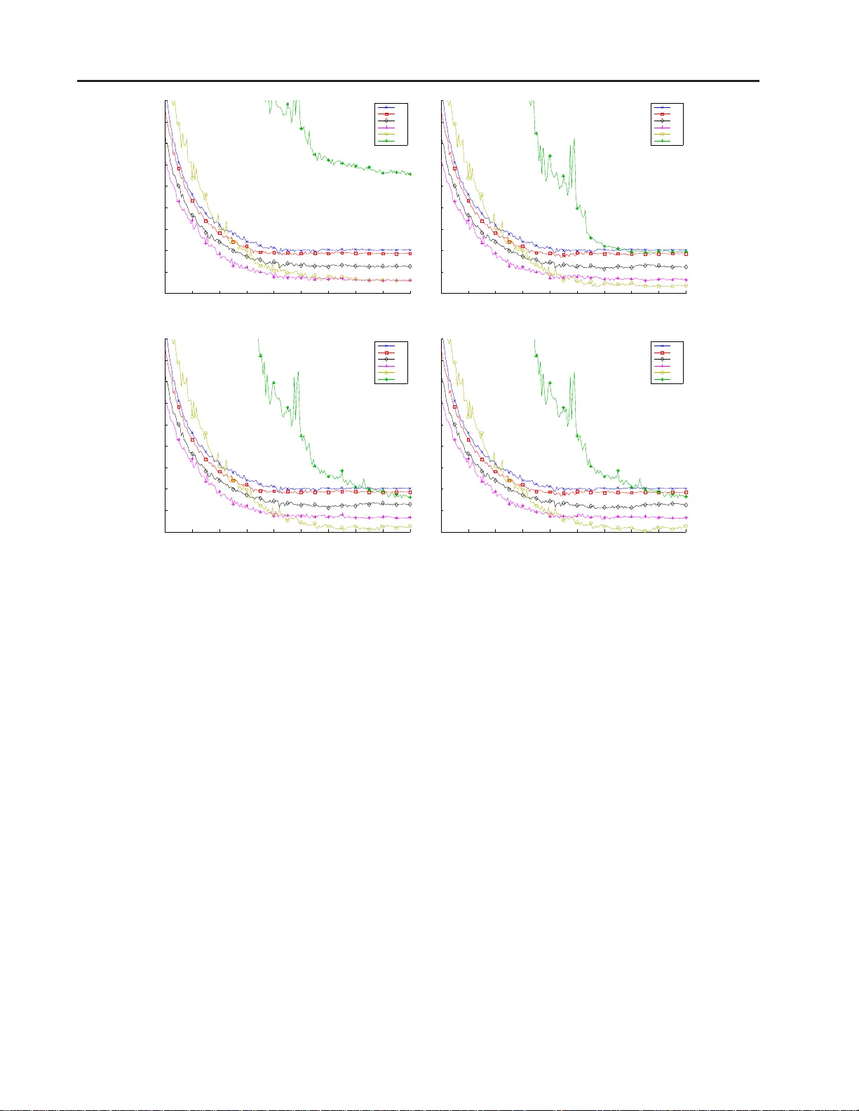
Single-Solution Hyperv olume Maximization and its use f or Impro ving Generali zation of Neural Networks Conrado S. Miranda C O N TAC T @ C O N R A D O M I R A N D A . C O M Fer nando J . V on Zuben VO N Z U B E N @ D C A . F E E . U N I C A M P . B R University of Campinas, Brazil Abstract This paper intro duces the hyper v olume maxi- mization with a single solution as an alternative to the mean loss minimization. The relation- ship between the tw o problems is proved throug h bound s on the cost fu nction when an optimal so- lution to on e of th e problem s is evaluated on th e other, with a hyper parameter to co ntrol the simi- larity between the two pro blems. This same hy - perpara meter allows higher weig ht to be placed on samples with higher loss when compu ting the hypervolume’ s gradie nt, wh ose norm alized ver- sion can r ange f rom the mean loss to the max loss. An experiment o n MNIST with a neur al network is used to validate the theory dev eloped, showing that th e hypervolume m aximization can behave similarly to the mean lo ss minimizatio n and can also provide better perfo rmance, result- ing on a 20% redu ction o f the classification error on the test set. 1. Intr oduction Many m achine learning algorith ms, inc luding neur al net- works, can b e divided into three pa rts: the model, which is used to describe or ap proximate the stru cture p resent in the tra ining d ata set; the loss func tion, which defin es how well an instance of the mo del fits th e samples; and the o p- timization method , which ad justs th e mo del’ s parameters to improve the e rror expressed by the loss function . Obvi- ously these thre e parts are related , and the genera lization capability o f the o btained solution depends on the ind i v id- ual merit of ea ch on e of the thr ee parts, and also on their interplay . Most of current research in machin e learning focuses on creating new models ( Bengio , 2 009 ; Goo dfello w et al. , 2016 ; K oller & Friedm an , 2009 ), for different appli- cations and data types, and n e w optimization meth- ods ( Bennett & Parrado-Hern ´ andez , 2006 ; Daup hin et al. , 2015 ; Duchi et al. , 2 011 ; Zeiler , 2012 ), which may allo w faster conv ergence, mo re robustness, and a better chance to escape from poor local minima. On th e other hand , many cost functions come from statis- tical models ( Bishop , 20 06 ), such as the qu adratic error, cross-entro py or variational bo und ( Kingma & W elling , 2013 ), although some terms of the cost related to regularization not necessarily have statistical b asis ( Cortes & V apnik , 1995 ; Miyato et al. , 20 15 ; Rifai et al. , 2011 ). When b uilding the total cost o f a sample set, we fre- quently sum the costs for each sample plus regulariz ation terms for th e whole dataset. Altho ugh this method ology is sound, it can be pr oblematic in real-world applications in volving more complex models. More specifically , if the learning problem is v ie we d from a multi-objective optimization (MOO) persp ecti ve as min- imization of the cost for each sample individually , then not ev ery efficient solution may be achieved by a conv ex com- bination of the costs ( Boyd & V andenb erghe , 2004 ) and Pareto-based solutions mig ht provide better results ( Freitas , 2004 ). An altern ati ve to minimiz ing the conve x com bi- nation is to maximize a metric known as the hyp erv ol- ume ( Zitzler et al. , 200 7 ), which c an be used to measure the quality of a set of samp les. As MOO algo rithms usu- ally search for many solutions with d if ferent tr ade-offs o f the objectives at the same time ( Deb , 2014 ), which can be used in an ensemble for in stance ( Chandra & Y ao , 2006 ), this ability to ev aluate the wh ole set of solutions instead of a single o ne made this metric wid ely used in MOO ( W agner et al. , 2007 ). The computation of the hype rv olume is NP-complete ( Beume et al. , 2009 ), making it hard to be used when there are m any objectiv es and candida te solutions. Nonetheless, in the par ticular case that a single candidate solution is b e- ing used, it can be computed in linear time with the number of objectives, wh ich makes its compu ting time equal to the Single-Solution Hyperv olume for Impr oving Generalization of NNs one associated with a conve x c ombination. Under the MOO p erspecti ve of having a single ob jecti ve function per s ample, in this p aper we de velop a theory lin k- ing th e maximiz ation of the single-so lution h ypervolume to the minimiza tion of the me an loss, in which the a verage of the cost over the tra ining sam ples is con sidered. W e pro- vide theoretical bo unds on the hyper v olume value in the neighbo rhood of an optimal solutio n to the me an loss and vice-versa, showing that these bo unds can be m ade arbi- trarily small su ch tha t, in th e limit, the optimal value for one prob lem is also optimal for the other . Moreover , we analyze the g radient o f the hy pervolume, showing th at it places more impo rtance to sam ples with higher cost. Since gradient optimization is an iterative process, th e hypervolume maximization imp lies an auto - matic reweighing of th e samp les at each itera tion. This reweighing allows the hypervolume gradient to range from the maximu m loss’ to the mea n loss’ g radient b y ch ang- ing a hyperpa rameter . It is also different from optimizing a linear combination of the mean and m aximum losses, as it also consider s the losses of intermediary samples. W e conjec ture that the g radient ob tained from the hyper- volume guides to improved models, as it is able to express a compr omise between fitting well the average sample and the worst samples. The a utomatic reweighing prevents the learning algo rithm f rom pursuing a quick reduction in the mean loss if it r equires a sign ificant increase in the loss o n already badly represented samples. W e perform an experiment to provid e both empirical evi- dence for th e conjectur e, showing that using the hyp erv ol- ume max imization reduces classification error when com- pared to the mean loss minimization, and validation for the theory developed. This p aper is organized as f ollo ws. Section 2 p rovides an overview o f multi-objective optim ization, properly charac- tering the ma ximization of the hyper v olume as a perfo r - mance indicato r for the lea rning system. Section 3 presen ts the theo retical developments o f th e p aper an d Sectio n 4 de- scribes the experiment pe rformed to validate the theo ry and provides e vidence fo r con jectures d e veloped in the paper . Finally , Sec tion 5 outlines conclu ding remark s and futu re research directions. 2. Multi-objectiv e optimization Multi-objective optimization (MOO) is a gen eralization of the traditional sing le-objectiv e optimization , where the p roblem is composed of m ultiple objective functions f i : X → R , i ∈ [ N ] , where [ N ] = { 1 , 2 , . . . , N } ( Deb , 2014 ). Using th e standard notation for MOO, the problem can be described by: min x ∈X f 1 ( x ) , . . . , min x ∈X f N ( x ) , (1) where X is the decision space and inclu des all con straints of the optimization . If so me of the o bjecti ves ha ve the same minima, then the redundant ob jecti ves can be ignored du ring optimiza- tion. Howe ver , if their min ima are dif ferent, for example f 1 ( x ) = x 2 and f 2 ( x ) = ( x − 1) 2 , then there is n ot a sin- gle optima l point, but a set o f different trade-offs betwee n the obje cti ves. A solution that establishes an optimal trad e- off, so that it is impossible to red uce one of the o bjecti ves without incr easing another, is said to b e efficient. The set of efficient solutions is called the Pareto set and its coun - terpart in the objective space is called the Pareto frontier . 2.1. Linear combination A common appro ach in op timization used to deal with multi-objec ti ve prob lems is to combine the objectives lin- early ( Boyd & V andenb erghe , 200 4 ; Deb , 2014 ), so that the problem becomes min x ∈X N X i =1 w i f i ( x ) , (2) where the weight w i ∈ R + represents the relative impor- tance given to objective i ∈ [ N ] . This approach is frequently found in learning with regular- ization ( Bishop , 20 06 ), where one objective is to decr ease the loss on the training set and ano ther is to d ecrease the model comp le xity , and th e mu ltiple objectives are com- bined with weights for the regularization terms to b alance the trade-off. Exa mples of this technique include soft- margin support vector m achines ( Cortes & V apnik , 1995 ), semi-superv ised m odels ( Rasmus et al. , 201 5 ), an d adver- sarial examples ( Miyato et al. , 2015 ), among many other s. Although the o ptimal solution of the linea rly combin ed problem is guaranteed to be efficient, it is on ly possible to achieve any ef ficient solution when th e objectives are con- vex ( Boyd & V andenb erghe , 20 04 ). This means that some desired solutions may not be achiev able b y p erforming a linear combin ation of the objectives and Pareto-b ased ap- proach es should be used ( Freitas , 2004 ), wh ich led to the creation of the hypervolume indica tor in MOO. 2.2. Hypervolume indicator Since the linear co mbination of o bjecti ves is not going to work p roperly on non-convex objecti ves, it is d esirable to in vestigate other forms of transforming the multi-ob jecti ve problem into a single-ob jecti ve one, which allows the stan- dard optimization tools to be used. Single-Solution Hyperv olume for Impr oving Generalization of NNs One com mon app roach in the multi-objective literature is to resort to the hypervolume in dicator ( Zitzler et al. , 2007 ), giv en by H ( z , X ) = Z Y 1[ ∃ x ∈ X : f ( x ) ≺ y ≺ z ]d y , (3) where z ∈ R N is the referen ce point, X ⊆ X , f ( · ) is the vector o btained by stackin g the ob jecti ves, ≺ is the dominan ce op erator ( Deb , 201 4 ), which is similar to th e < com parator and can b e defined as x ≺ y ⇔ ( x 1 < y 1 ) ∧ . . . ∧ ( x N < y N ) , and 1[ · ] is the indicator operator . The problem then becomes m aximizing the hyp erv olume over the domain, and this optimizatio n is ab le to achieve a larger number o f e f ficient p oints, without req uiring con - vexity of the Pareto frontier ( Auger et al. , 2009 ). Although the hy pervolume is frequen tly used to analyze a set of candidate solutions ( Zitzler et al. , 2003 ) and led to state-of-the- art algorith ms for MOO ( W agner et al. , 2007 ), it can be expen si ve to compute as it is NP-c omplete ( Beume et al. , 200 9 ). However , for a single solution, that is, if | X | = 1 , it can be computed in linea r time and its logarithm can be written as: log H ( z , { x } ) = N X i =1 log( z i − f i ( x )) , (4) giv en that f i ( x ) < z i . Among the many prop erties of the hypervolume, two mu st be highlighted in this paper . First, the hypervolume is monoto nic in the ob jecti ves, which mea ns that any r educ- tion of any objectiv e cau ses the hyp erv olume to inc rease, which in turn is alig ned with the loss minimization . T he maximum of the single- solution hyper v olume is a po int in the Pareto set, which means that the solution is ef ficient. The second proper ty is that, like the linear combination , it also maintains som e shape inform ation from the objectives. If th e objectives are conv ex, th en their linea r combina tion is con vex and the hyp erv olume is con ca ve, since − f i ( x ) is co nca ve and the logar ithm of a concave function is co n- cav e. 2.3. Loss minimization A common objec ti ve in machine learning is the minimiza- tion of some loss f unction l : D × Θ → R over a giv en data set S = { s 1 , . . . , s N } ⊂ D . Note that this no tation includes both super vised and un supervised learning, as the space D can include both the samp les and their targets. For simplicity , let l i ( θ ) : = l ( s i , θ ) , so that the specific data set does not have to be consider ed. Defining f i : = l i and X : = Θ , the loss min imization can be wr itten as Eq. ( 1 ). Just like in oth er areas of o ptimiza- tion, the usual approac h to solve these prob lems in mach ine learning is the use of a linear comb ination of the objec ti ves, as discussed in Sec. 2.1 . Howev er , a s also discussed in Sec. 2.1 , this appr oach limits the numb er of solutio ns that can be ob tained if the losses ar e n ot convex, which m oti- vates the use of the hy perv olume indicator . Since the ob jecti ves differ only in the samples used f or the loss function and considering that all samples have equal importan ce 1 , the Nad ir po int z can h a ve the sam e value for all o bjecti ves so th at the solution found is b alanced in the losses. This value is g i ven by the parameter µ , so th at z i = µ, ∀ i ∈ [ N ] . Then the prob lem becomes maximizing log H ( µ 1 N , { θ } ) in relation to θ , where 1 N is a vector of ones with size N and log H ( · ) is defined in Eq. ( 4 ). 3. Theory of the single-solution hype rvolume In this section, we develop the theor y linking the single- solution h ypervolume maximization to the minimization of the mean lo ss, wh ich is a common optimization objec- ti ve. First, we define th e r equirements that a loss functio n must satisfy and describe the two optimization pro blems in Sec. 3.1 . T hen, g i ven an op timal solutio n to one problem, we will show in Sec. 3.2 boun ds on the loss o f optimal- ity of the other prob lem in th e neigh borhood of the given solution and will show th at these bou nds can be ma de ar- bitrarily small b y changing the reference poin t. Finally in Sec. 3.3 , we will sh o w how to transfor m the gradie nt of the hypervolume to a f ormat similar to a conv ex combina- tion of the gradients of each loss , which will be used in the experiments of Sec. 4 to show the advantage of using the hypervolume maximization. 3.1. Definitions In order to elaborate the theory , we must d efine so me te rms that will be used on the results. Definition 1 (Lo ss Fun ction) . Let Θ be an ope n subset of R n . Let l : Θ → R be a continuo usly differ entiable fun c- tion. Then l is a loss function if th e following c onditions hold: • The loss is b ounded everywher e, that is, | l ( θ ) | < ∞ for all θ ∈ Θ ; • The gradient is bo unded everywhere , that is, k∇ l ( θ ) k < ∞ for all θ ∈ Θ . The op enness of Θ simplifies the th eory as we do not ha ve to worry about op tima on th e b order , which are hard er to deal with d uring pro ofs. Howe ver , the theor y can be ad - 1 This is the same motiv ation for using the uniform mean loss. If prior importance is av ailable, it can be used to define the value of z , like it w ould be used to define w in the weighted mean loss. Single-Solution Hyperv olume for Impr oving Generalization of NNs justed so that Θ can be clo sed and points on the bord er are allowed to ha ve infinite loss. Definition 2 (Mean loss pro blem) . Let Θ be an o pen sub set of R n . Let L = { l 1 , . . . , l N } b e a set of lo ss func tions defined over Θ . Then the mean loss J m : Θ → R and its associated minimization pr o blem are defined as min θ ∈ Θ J m ( θ ) , J m ( θ ) = 1 N N X i =1 l i ( θ ) . (5) Definition 3 (Hyper v olume prob lem) . Let Θ be an op en subset o f R n . Let L = { l 1 , . . . , l N } b e a set of lo ss func- tions defined over Θ . Let µ be given such that ther e exists some θ ∈ Θ that satisfies µ > l ( θ ) for all l ∈ L . Let Θ ′ = { θ | θ ∈ Θ , µ > l ( θ ) , ∀ l ∈ L } . Then the hyper- volume H : R × Θ ′ → R a nd its associated maximiza tion pr o blem ar e define d as max θ ∈ Θ ′ H ( µ, θ ) , H ( µ, θ ) = N X i =1 log( µ − l i ( θ )) . (6) Note th at the h ypervolume defined h ere is a simplifica- tion of the function defined in Eq. ( 4 ), so that H ( µ, θ ) : = log H ( µ 1 N , { θ } ) . 3.2. Connection between J m ( θ ) and H ( µ, θ ) Using th e definitions in the last section , we can n o w state bound s when app lying th e o ptimal solution of a prob lem to the othe r . The pro ofs are not present in this s ection in order to a void cluttering, b ut are provided in Appendix A . Theorem 1. Let Θ be a n op en subset o f R n . Let L = { l 1 , . . . , l N } be a set of loss functio ns defined over Θ . Let θ ∗ ∈ Θ be a local m inimum of J m ( θ ) an d let ǫ > 0 such that θ ∗ + δ ∈ Θ for all k δ k ≤ ǫ . Let C 1 , C 2 and C 3 be such that C 1 ≤ l i ( θ ∗ + δ ) ≤ C 2 and k∇ l i ( θ ∗ + δ ) k ≤ C 3 for all i ∈ [ N ] an d k δ k ≤ ǫ . Let ν > 0 . Then ther e is some ǫ ′ ∈ (0 , ǫ ] such that H ( µ, θ ∗ + δ ) ≤ H ( µ, θ ∗ ) + ν C 3 ǫ ′ N µ − C 2 , (7) for all k δ k ≤ ǫ ′ and µ > γ , wher e γ = max  C 2 , (1 + ν ) C 2 − C 1 ν , C 2 − (1 − ν ) C 1 ν  . (8) Theorem 2. Let Θ be a n op en subset o f R n . Let L = { l 1 , . . . , l N } be a set of loss functio ns defined over Θ . Let θ ∗ ∈ Θ be a local maximum of H ( µ, θ ) fo r some µ a nd let ǫ > 0 such that θ ∗ + δ ∈ Θ for all k δ k ≤ ǫ . Let C 1 , C 2 and C 3 be such that C 1 ≤ l i ( θ ∗ + δ ) ≤ C 2 and k∇ l i ( θ ∗ + δ ) k ≤ C 3 for all i ∈ [ N ] a nd k δ k ≤ ǫ . Then ther e is some ǫ ′ ∈ (0 , ǫ ] such that J m ( θ ∗ + δ ) ≥ J m ( θ ∗ ) − ν C 3 ǫ ′ (9) for all k δ k ≤ ǫ ′ , wher e ν = max  µ − C 1 µ − C 2 − 1 , 1 − µ − C 2 µ − C 1  . (10) Note that ν in Eqs. ( 7 ) and ( 9 ) is multiplying the regular bound s due to the co ntinuous d if ferentiability of the func - tions. If ν ≥ 1 , then the knowledge that a given θ ∗ is op- timal in the other p roblem does not provide any additional informa tion. Howe ver , ν can be mad e arbitr arily small by making µ large, so increasing µ allows more inf ormation to b e shared among the problems as their lo ss surfaces be- come closer . One practica l applica tion of these theorem s is that, given a value ν ∈ (0 , 1) and a region Ω ⊆ Θ , we ca n chec k wheth er the refer ence point µ is large enough for all θ ∈ Ω . If it is, then optimizin g H ( µ, θ ) over Ω is similar to o ptimizing a boun d on J m ( θ ) aroun d the optimal solution and vice- versa, with the difference be tween the boun d and the real value v anishing as ν gets smaller and µ gets larger . 3.3. Gradient of H ( µ, θ ) in t he limit The gradient of the h ypervolume, as defined in Eq . ( 6 ), is giv en by: ∇ θ H ( µ, θ ) = − N X i =1 1 µ − l i ( θ ) ∇ l i ( θ ) . (11) Note tha t usin g the hy pervolume automatically places more importan ce on samples with h igher loss during optimiza- tion. W e conjectur e that this au tomatic control of re le vance is beneficial for learnin g a function with better gener alization, as the model will be forced to focus more of its capacity on samples th at it is not able to represen t well. Moreover , the hyperp arameter µ provid es some contr ol over how m uch difference o f impo rtance can be placed on the sam ples, as will be shown below . Th is is similar to soft-margin suppo rt vector machin es ( Cortes & V apnik , 1 995 ), where we can change th e regulariza tion h yperparameter to co ntrol how much the margin can be reduced in order to better fit mis- classified samples. W e provid e empirical evidence for this conjecture in Sec. 4 . For a gi ven θ , this g radient can change a lot by changing µ , which should be avoided during the optimization in real scenarios. In o rder to stabilize the g radient and make it similar to the g radient of a conve x comb ination of the ob- jectiv e’ s gradients, we can use ∇ θ H ( µ, θ ) P N i =1 1 µ − l i ( θ ) = − N X i =1 w i ∇ l i ( θ ) , w i = 1 µ − l i ( θ ) P N j =1 1 µ − l j ( θ ) , (12) Single-Solution Hyperv olume for Impr oving Generalization of NNs so that w i ≥ 0 for all i ∈ [ N ] and P N i =1 w i = 1 . When the referen ce µ eithe r beco mes large or close to its allowed lower bound, this normalized grad ient presen ts in- teresting behaviors. Lemma 3. Let Θ be an o pen sub set of R n . Let L = { l 1 , . . . , l N } be a set of loss functio ns defined over Θ . Let θ ∈ Θ . Then lim µ →∞ ∇ θ H ( µ, θ ) P N i =1 1 µ − l i ( θ ) = −∇ J m ( θ ) . (13) Pr oo f. Let α i : =  1 µ − l i ( θ )  /  P N j =1 1 µ − l j ( θ )  . Then lim µ →∞ α i = 1 N , which gives the hypervolume limit as: lim µ →∞ ∇ θ H ( µ,θ ) P N i =1 1 µ − l i ( θ ) (14a) = lim µ →∞ − P N i =1 α i ∇ l i ( θ ) = − ∇ J m ( θ ) . (14b)  Lemma 4. Let Θ be an o pen sub set of R n . Let L = { l 1 , . . . , l N } be a set of loss functio ns defined over Θ . Let θ ∈ Θ . Let ∆( θ ) : = max i ∈ [ N ] l i ( θ ) a nd S = { i | i ∈ [ N ] , ∆( θ ) = l i ( θ ) } . Th en lim µ → ∆( θ ) + ∇ θ H ( µ, θ ) P N i =1 1 µ − l i ( θ ) = − 1 | S | X i ∈ S ∇ l i ( θ ) (15) Pr oo f. Let α i : =  1 µ − l i ( θ )  /  P N j =1 1 µ − l j ( θ )  . Then lim µ → ∆( θ ) + α i = 1[ i ∈ S ] / | S | , which giv es the hyp er - volume limit as: lim µ → ∆( θ ) + ∇ θ H ( µ,θ ) P N i =1 1 µ − l i ( θ ) (16a) = lim µ → ∆( θ ) + − P N i =1 α i ∇ l i ( θ ) = − 1 | S | P i ∈ S ∇ l i ( θ ) . (16b)  As shown in Sec. 3.2 , the mea n loss and hyper v olume prob- lems become closer as µ increases. In the limit, the n ormal- ized gr adient fo r the hyper v olume beco mes equ al to the gradient of the mean lo ss. On the o ther hand, when µ is close to its lower boun d ∆( θ ) , it become s the mean gradi- ent of all the loss fu nctions with maximum value. In partic- ular , if | S | = 1 , that is, only one loss has m aximal value at some θ , then the n ormalized grad ient for the hypervolume becomes equal to the gradient of the maximum loss. 4. Experimental validation T o validate the u se of the sing le-solution hypervolume in - stead of the mean loss f or train ing neur al networks, we used a LeNet- lik e network on the MNIST dataset ( LeCun et al. , 1998 ). This ne tw ork is com posed of three laye rs, all with ReLU acti vation, where th e first two layers ar e conv olu- tions with 20 and 50 filters, resp ecti vely , of size 5x5, both followed by max-p ooling of size 2x2, while the last layer is fully connec ted and comp osed of 500 hidden units with dropo ut p robability of 0.5. The learning was perf ormed by gradient descent with base learnin g rate of 0 .1 and momen - tum o f 0.9, which were selected using the validation set to provide the best perf ormance for th e mean loss optimiza- tion, an d minibatch es of 500 samples. After 20 iteratio ns without improvemen t on the validation error, the learn ing rate is re duced by a factor of 0.1 until it r eaches the value of 0.001 , after whic h it is kept constant until 200 iterations occurre d. For t he hypervolume, instead of fixing a single v alue for µ , which wou ld r equire it to be large as the neural network has high loss when initialized, we allowed µ to ch ange as µ = (1 + 10 ξ ) max i l i ( θ ) (17) so that it can follow the improvement on the loss functions, where i are the samples in the min i-batch and the param - eters’ gradien ts are not backpr opagated through µ . Any value ξ ∈ R ∪ {∞} p rovides a valid referen ce point and larger values make th e pro blem closer to using the mean loss. W e tested ξ ∈ Ξ = {− 4 , − 3 , − 2 , − 1 , 0 , ∞} , where ξ = ∞ represents th e mean loss, an d allowed for schedul- ing of ξ . In this ca se, bef ore decreasin g the learning rate when the learn ing stalled, ξ is incremen ted to the n e xt value in Ξ . W e have also consider ed the possibility of ∞ / ∈ Ξ , to ev aluate the effect of not using the mea n together with th e schedule. Figure 1 shows the results f or each scenario co nsidered. First, note th at using ξ 0 = 0 provided results close to the mean loss thro ughout the iterations o n all scenarios, which empirically validates the theory that large values of µ m akes maximization of the hyp erv olume similar to min- imization of the mean loss and provides evidence that µ does not have to be so large in comparison to the loss func - tions for this to happ en. More ov er , Figs. 1c and 1d are sim- ilar for all values of ξ 0 , which provides further evidence that ξ = 0 is large enough to ap proximate the mean loss well, as includin g ξ = ∞ in the sche dule or not does n ot change the perfor mance. On the other hand, ξ 0 = − 4 w as not able to provide go od classification by itself, requiring the use of o ther values of ξ to ach ie ve an error r ate similar to the mean loss. Although it is a ble to get better r esults with the help o f sch edule, as shown in Figs. 1c and 1d , th is prob ably is du e to the o ther Single-Solution Hyperv olume for Impr oving Generalization of NNs 20 40 60 80 100 120 140 160 180 200 60 70 80 90 100 110 120 130 140 150 Iteration Classification error ∞ 0 -1 -2 -3 -4 (a) Ξ = { ξ 0 } 20 40 60 80 100 120 140 160 180 200 60 70 80 90 100 110 120 130 140 150 Iteration Classification error ∞ 0 -1 -2 -3 -4 (b) Ξ = { ξ 0 , ∞} 20 40 60 80 100 120 140 160 180 200 60 70 80 90 100 110 120 130 140 150 Iteration Classification error ∞ 0 -1 -2 -3 -4 (c) Ξ = { ξ 0 , . . . , 0 } 20 40 60 80 100 120 140 160 180 200 60 70 80 90 100 110 120 130 140 150 Iteration Classification error ∞ 0 -1 -2 -3 -4 (d) Ξ = { ξ 0 , . . . , 0 , ∞} Figure 1. Mean numb er of misclassified samples in the test set over 20 runs for different initial v alues ξ 0 and t raining strategies, with ξ = ∞ representing the mean loss and Ξ r epre senting the schedule of value s of ξ used when no impro veme nt is observed. values of ξ them selv es instead of ξ 0 = − 4 providin g di- rect benefit, as it achiev ed an error similar to the mean loss when no schedule e xcept for ξ = ∞ was used, as sho wn in Fig. 1b . Th is indicates that too much pressur e on the sam- ples with high lo ss is not beneficial, wh ich is explained b y the optimiza tion becom ing closed to min imizing the max- imum loss, as discussed in Sec. 3.3 , thus ign oring most of the samples. When optimizing the hypervolume starting f rom ξ 0 ∈ {− 1 , − 2 , − 3 } , all scenarios showed improvemen ts on the classification erro r , with all the differences after conver - gence between op timizing the hypervolume and th e mean loss b eing statistically significan t. Moreover , better re sults were ob tained when the schedule started from a smaller value of ξ 0 . This provides evidence to the conjecture in Sec. 3. 3 that placing higher pressure on samples with high loss, which is repr esented by higher values o f w i in Eq. ( 12 ), is b eneficial an d might help the network to achieve h igher g eneralization, but also w arns that too much pressure can be prejudicial as the resu lts for ξ 0 = − 4 show . Furthermo re, Fig. 1 indicates that, e ven if this p ressure is kept thr oughout the training, it mig ht improve th e results compare d to using only the mean loss, b ut that reducing the pressure as the training pr ogresses imp roves the results. W e suspect th at reducing the pr essure allo ws rare samples that cannot be well learn ed b y the mod el to be less relev ant in fa vor of more common samples, which im proves the gen - eralization overall, and that the initial p ressure allo wed the model to learn better r epresentations for the data, as it was forced to consider more the bad samples. The presen ce of these rare and bad samples also explain why ξ 0 = − 4 pro- vided bad results, as the learning algor ithm foc used main ly on sam ples th at canno t be approp riately learnt b y the mo del instead of focusing on the more representative ones. T able 1 provides the error s for th e mean loss, represen ted by ξ 0 = ∞ , and f or h ypervolume with ξ 0 = − 3 , which p re- sented the best impr ov ements. W e used the classification error on the validation set to select th e parameters used for computin g the classification error on the test set. I f no t used alone, with either sched uling or mean or both, maximizing the hypervolume l eads to a reduction of at least 20% in the Single-Solution Hyperv olume for Impr oving Generalization of NNs T able 1. Mean number of misclassified samp les in the test se t ov er 20 runs. The differences between ξ 0 = ∞ and ξ 0 = − 3 are statistically significant ( p ≪ 0 . 0 01 ). ξ 0 Schedule Mean Errors Reductio n ∞ 80.8 − 3 X X 67.5 16.5% − 3 X X 64.2 20.5% − 3 X X 62.9 22.2 % − 3 X X 63.4 21.6% classification er ror without ch anging the convergence tim e significantly , as observed in Fig. 1 , which motiv ates its use in real prob lems. 5. Conclusion In this paper, we introduced the idea of using the hypervol- ume with a single s olution as an optimization objective and presented a theory fo r its use. W e showed how an optimal solution for the hyper v olume relates to the mean loss prob- lem, where we tr y to minimize the a verage of the lo ss es for each sample, and vice-versa, providin g bounds on the neighbo rhood of the o ptimal p oint. W e also showed how the g radient of the hy pervolume behaves when chan ging the reference point an d how to stabilize it f or practical ap- plications. This analysis raised the conjecture that using the hypervol- ume in machine learn ing might result in better models, as the hyper v olume’ s gradien t is co mposed of an auto mati- cally weighted average o f th e g radient for each sample with higher weights repr esenting hig her losses. This weighting makes the learning algo rithm focu s more on sam ples that are not well repr esented by the current set of param eters ev en if it mea ns a slower red uction of the mean loss. Hen ce, it forces the learning algorithm to search for re gions where all samples can be well represented , avoiding early com- mitment to less promising regions. Both the theor y a nd the conjecture were validated in an e x- periment with MNIST , where using the hy pervolume max- imization led to a reductio n of 20% in the classification er- rors in comparison to the mean loss minimization. Future research sh ould f ocus on studyin g mor e theor eti- cal and empirical prope rties of the single-solution hyper- volume maximization , to provid e a solid explanation fo r its impr ov ement over the mea n loss and in which scen ar - ios this could be expected . Th e robustness of the method should also be in vestigated, as to o much noise or the p res- ence of ou tliers might cause large losses, which op ens the possibility of in ducing the learner to place high imp ortance on these losses in detrimen t of more common cases. A. Proofs A.1. Proof of Th eorem 1 Lemma 5. Let Θ be an o pen sub set of R n . Let L = { l 1 , . . . , l N } be a set of loss functio ns defined over Θ . Let θ ∗ ∈ Θ be a local minimum o f J m ( θ ) . Then there is some ǫ > 0 such tha t, for all ∆ with k ∆ k ≤ ǫ , we have θ ∗ + ∆ ∈ Θ and P N i =1 ∇ l i ( θ ∗ + ∆) · ∆ ≥ 0 . Pr oo f. Since Θ is o pen, there is some σ > 0 su ch that θ ∗ + δ ∈ Θ for all k δ k ≤ σ . Since θ ∗ is a local minim um of J m ( θ ) , there is some ǫ ′ ∈ (0 , σ ] suc h that J m ( θ ∗ + δ ) ≥ J m ( θ ∗ ) fo r all k δ k ≤ ǫ ′ . Given som e δ 6 = 0 , from the mean value theorem we have that J m ( θ ∗ + δ ) − J m ( θ ∗ ) = ∇ J m ( θ ∗ + ∆) · ∆ /c ( δ ) ( 18) for some c ( δ ) ∈ (0 , 1) , where ∆ = c ( δ ) δ . From the o pti- mality , we have 0 ≤ J m ( θ ∗ + δ ) − J m ( θ ∗ ) = 1 N N X i =1 ∇ l i ( θ ∗ + ∆) · ∆ /c ( δ ) . (19) If δ = 0 , then the eq uality is tr i v ially satisfied. Let κ = min k δ k≤ ǫ ′ c ( δ ) . Then defining ǫ = ǫ ′ κ completes the proof.  Lemma 6. Let Θ be an o pen sub set of R n . Let L = { l 1 , . . . , l N } be a set of loss functio ns defined over Θ . Let θ ∈ Θ an d ǫ > 0 such that θ + δ ∈ Θ fo r all k δ k ≤ ǫ . Let ν > 0 , β i ( δ ) : = 1 µ − l i ( θ + δ ) and α i ( δ ) : = β i ( δ ) P N j =1 β j ( δ ) . Let C 1 and C 2 be such th at C 1 ≤ l i ( θ + δ ) ≤ C 2 for all i ∈ [ N ] and k δ k ≤ ǫ . Then | N α i ( δ ) − 1 | ≤ ν (20) for all i ∈ [ N ] , k δ k ≤ ǫ and µ > γ , wher e γ = max n C 2 , (1+ ν ) C 2 − C 1 ν , C 2 − (1 − ν ) C 1 ν o . Pr oo f. For Eq. ( 20 ) to hold, we must have N α i ( δ ) − 1 ≤ N max i,δ α i ( δ ) − 1 ≤ ν (21a) N α i ( δ ) − 1 ≥ N min i,δ α i ( δ ) − 1 ≥ − ν. (2 1b) Using the bound s C 1 and C 2 , we can bou nd β i ( δ ) as: max i,δ β i ( δ ) ≤ 1 µ − C 2 , min i,δ β i ( δ ) ≥ 1 µ − C 1 . (22) Hence, we have that Eq. ( 21a ) can be satisfied by: 1 µ − C 2 N 1 µ − C 1 ≤ 1 + ν N ⇒ (1 + ν ) C 2 − C 1 ν ≤ µ (23) Single-Solution Hyperv olume for Impr oving Generalization of NNs and Eq. ( 21b ) can be satisfied by: 1 µ − C 1 N 1 µ − C 2 ≥ 1 − ν N ⇒ C 2 − (1 − ν ) C 1 ν ≤ µ. (24) The additional value in the d efinition of γ guarantees that µ does not beco me inv a lid.  Pr oo f of Theorem 1 . From the mean value theorem, for any δ we ha ve that H ( µ, θ ∗ + δ ) − H ( µ, θ ∗ ) (25a) = − N X i =1 1 µ − l i ( θ ∗ + ∆) ∇ l i ( θ ∗ + ∆) · δ (25b) for some c ( δ ) ∈ (0 , 1) , where ∆ = c ( δ ) δ . Let ǫ 1 be the value defined in Lemma 5 and define ǫ ′ = min { ǫ, ǫ 1 } . Then restricting k δ k ≤ ǫ ′ implies that k ∆ k ≤ ǫ 1 and that the results in Lemma 5 h old. Therefore P N i =1 ∇ l i ( θ ∗ + ∆) · ∆ ≥ 0 for all k δ k ≤ ǫ ′ . Then, using Lemma 6 , the difference between the hy per - volumes can be b ounded as: H ( µ, θ ∗ + δ ) − H ( µ, θ ∗ ) P N j =1 β j (∆) = − N X i =1 α i (∆) ∇ l i ( θ ∗ + ∆) · δ (26a) ≤ − 1 N N X i =1 ( N α i (∆) − 1 ) ∇ l i ( θ ∗ + ∆) · δ (26b) ≤ 1 N N X i =1 | N α i (∆) − 1 |k∇ l i ( θ ∗ + ∆) kk δ k (26c) ≤ ν C 3 ǫ ′ . (26d) Using the fact that β i is upp er bou nded accord ing to Eq. ( 22 ), we achieve the final boun d.  A.2. Proof of Th eorem 2 Lemma 7. Let Θ be an o pen sub set of R n . Let L = { l 1 , . . . , l N } be a set of loss functio ns defined over Θ . Let θ ∈ Θ and ǫ > 0 such tha t θ + δ ∈ Θ for all k δ k ≤ ǫ . Let β i ( δ ) : = 1 µ − l i ( θ + δ ) and α i ( δ ) : = β i ( δ ) P N j =1 β j ( δ ) . Let C 1 and C 2 be such that C 1 ≤ l i ( θ + δ ) ≤ C 2 for all i ∈ [ N ] a nd k δ k ≤ ǫ . Then | N α i ( δ ) − 1 | ≤ ν (27) for all i ∈ [ N ] an d k δ k ≤ ǫ , where ν = max n µ − C 1 µ − C 2 − 1 , 1 − µ − C 2 µ − C 1 o . Pr oo f. For Eq. ( 27 ) to hold, we must satisfy the conditions in Eq. ( 2 1 ). Using the bo unds C 1 and C 2 , we can boun d β i ( δ ) as in Eq . ( 22 ). Hen ce, we have that Eq. ( 23 ) and Eq. ( 24 ) can be satisfied by: µ − C 1 µ − C 2 − 1 ≤ ν, 1 − µ − C 2 µ − C 1 ≤ ν. (28 )  Lemma 8. Let Θ be an o pen sub set of R n . Let L = { l 1 , . . . , l N } be a set of loss functio ns defined over Θ . Let θ ∗ ∈ Θ be a loca l maximum of H ( µ, θ ) for some µ . Then ther e is some ǫ > 0 such that, for all ξ ∈ (0 , ǫ ] and ∆ with k ∆ k ≤ ξ , we have θ ∗ + ∆ ∈ Θ and N X i =1 ∇ l i ( θ ∗ + ∆) · ∆ ≥ − ν C 3 ξ N , (29 ) wher e C 1 , C 2 and C 3 ar e s uch that C 1 ≤ l i ( θ ∗ + ∆) ≤ C 2 and k∇ l i ( θ ∗ + ∆) k ≤ C 3 for all i ∈ [ N ] and k ∆ k ≤ ξ and ν = max n µ − C 1 µ − C 2 − 1 , 1 − µ − C 2 µ − C 1 o . Pr oo f. Given som e δ , from the mean value theorem we have that Eq . ( 25 ) hold s for some c ( δ ) ∈ (0 , 1 ) , where ∆ = c ( δ ) δ . Since Θ is open, there is s ome σ > 0 such that θ ∗ + δ ∈ Θ for all k δ k ≤ σ . Since θ ∗ is a local max imum of H ( µ, θ ) , there is some ǫ ′ ∈ (0 , σ ] such that H ( µ, θ ∗ + δ ) ≤ H ( µ, θ ∗ ) for all k δ k ≤ ǫ ′ . Let κ = min k δ k≤ ǫ ′ c ( δ ) and define ǫ = ǫ ′ κ . Let ξ ∈ (0 , ǫ ] an d k ∆ k ≤ ξ . Usin g Lemma 7 , we hav e that 0 ≥ c ( δ )( H ( µ, θ ∗ + δ ) − H ( µ, θ ∗ )) P N j =1 β j (∆) (30a) = − N X i =1 α i (∆) ∇ l i ( θ ∗ + ∆) · ∆ (30b) ≥ − 1 N P N i =1 | ( N α i (∆) − 1 ) |k∇ l i ( θ ∗ + ∆) kk ∆ k − 1 N P N i =1 ∇ l i ( θ ∗ + ∆) · ∆ ! (30c) ≥ − ν C 3 ξ − 1 N N X i =1 ∇ l i ( θ ∗ + ∆) · ∆ , (30d) which gives th e bound.  Pr oo f of Theorem 2 . Giv en some δ , fro m th e mean v alue theorem we ha ve that Eq. ( 18 ) ho lds f or some c ( δ ) ∈ (0 , 1) , where ∆ = c ( δ ) δ . Let ǫ 1 > 0 be the value defined in Lemma 8 and define ǫ ′ = min { ǫ, ǫ 1 } . Th en restricting k δ k ≤ ǫ ′ implies th at k ∆ k ≤ ǫ 1 and that th e results in L emma 8 hold. Therefor e, let ξ = ǫ ′ and we have that P N i =1 ∇ l i ( θ ∗ + ∆) · ∆ ≥ − ν C 3 ǫ ′ N , which proves the bou nd.  Single-Solution Hyperv olume for Impr oving Generalization of NNs Acknowledgeme nts W e would like to thank CNPq and F APESP f or the financial support. Refer ences Auger, A., Bader, J., Brockhoff, D., and Zitzler , E. Theor y of the hypervolume ind icator: optima l µ -distributions and the c hoice of the ref erence p oint. In Pr oceedings of the tenth ACM S IGEV O workshop on F oun dations of genetic algorithms , pp. 87–102 . AC M, 2009. Bengio, Y . Learning d eep ar chitectures for AI. F oun dations and T r ends R  in Machine Learning , 2(1):1–1 27, 200 9. Bennett, K. P . and Parrado -Hern ´ andez, E. The interp lay of optimization and machine learn ing research. Th e Jour - nal of Machine Learning Resear ch , 7:126 5–1281, 2 006. Beume, N., Fonseca, C. M., L ´ opez-Ib ´ a ˜ nez, M., Paquete, L., and V ahrenh old, J. On the c omplexity of computing the hyper v olume in dicator. Ev olutionary Computa tion, IEEE T ransactions on , 13(5) :1075–108 2, 2009 . Bishop, C . M. P attern Recognition and Machine Learning . Springer, 2006. Boyd, S. P . a nd V ande nberghe, L. Conve x Optimization . Cambridge University Press, 2004. Chandra, A. and Y ao, X. Ensemble learning u sing multi- objective ev olutionary alg orithms. J o urnal o f Mathemat- ical Modelling and Algorithms , 5(4):41 7–445, 2006. Cortes, C. an d V apn ik, V . Support-vector networks. Ma - chine Learning , 20(3):273– 297, 1995 . Dauphin, Y ., de Vr ies, H., and Bengio, Y . Equilibrated adaptive learnin g rates f or non-co n vex optimization. I n Advance s in N eural I nformation Pr o cessing Systems , pp. 1504– 1512, 2 015. Deb, K. Multi-objec ti ve optimization. In Sea r ch method- ologies , pp. 403–449 . Sprin ger , 2014. Duchi, J., Hazan, E. , and Singer , Y . Adap ti ve subg radient methods for online learning and stochastic optimization. The Journal of Machine Learning Resear ch , 1 2:2121– 2159, 2011 . Freitas, A. A . A critical revie w of multi-o bjecti ve optimiza- tion in d ata mining: A position paper . SIGKDD Exp lor . Newsl. , 6(2):77–8 6, 2004 . Goodfellow , I., Bengio, Y ., and Courv ille, A. Dee p learn - ing. Book in pr eparation for MIT Press, 2016. URL http://goodf eli.github.io/dlboo k/ . Kingma, D. P . an d W elling, M. Auto-enc oding v ariational Bayes. arXiv pr eprint arXiv:131 2.6114 , 20 13. K oller , D. and Friedman, N. Pr obabilistic Graphical Mod- els: Principles and T echniqu es . MIT press, 2009 . LeCun, Y ., Bottou, L., Bengio, Y ., and Haffner, P . Gradient- based learning applied to do cument recognition . Pr o- ceedings of the IEEE , 86(11 ):2278–23 24, 199 8. Miyato, T ., Maed a, S., Koyama, M., Nakae, K. , and Ishii, S. Distributional smoothing by virtual adversarial exam- ples. arXiv pr eprint arXiv:1507.0 0677 , 201 5. Rasmus, A., Berglun d, M., Ho nkala, M., V alpola, H., and Raiko, T . Sem i-supervised learn ing with ladder net- works. In Advances in Neural Information P r ocessing Systems , pp. 3532– 3540, 2 015. Rifai, S., V incent, P ., Muller , X., Glorot, X., and Ben gio, Y . Contractive auto-en coders: Explicit in variance du ring feature extraction . I n Pr ocee dings o f th e 28th Intern a- tional Confer ence on Machine Learning (ICML-11 ) , pp. 833–8 40, 2 011. W agner, T ., Beume, N. , and Naujoks, B. Pareto-, aggregation- , and in dicator-based m ethods in m any- objective o ptimization. I n Ob ayashi, S., Deb, K., Poloni, C., Hiroyasu, T . , and Mur ata, T . ( eds.), Evo lution- ary Multi-Criterion Optimizatio n , volume 440 3 of Lec- tur e Notes in Comp uter Science , p p. 742–7 56. S pringe r , 2007. Zeiler , M. D. Adad elta: An adaptive learning rate m ethod. arXiv pr eprint arXiv:1212 .5701 , 2 012. Zitzler , E. , Thiele, L., Laumanns, M. , Fonseca, C. M., and Da Fonseca, V . G. Performa nce Assessment of Multiob- jectiv e Optimizers: An Analysis and Re view . Evolution- ary Computation, IEEE T r ansaction s on , 7(2):1 17–132, 2003. Zitzler , E., Brockh of f, D., and Thiele, L. The hypervolume indicator r e visited: O n the d esign of Pareto-co mpliant indicators via weigh ted integration. In Evo lution- ary mu lti-criterion optimization , pp. 862 –876. Springer, 2007.