Comparative evaluation of state-of-the-art algorithms for SSVEP-based BCIs

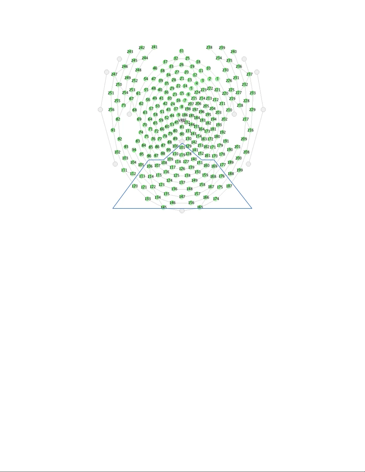
TECHNICAL REPOR T - ARXIV .ORG J ANU AR Y 2016 1 Comparati v e e v aluation of state-of-the-art algorithms for SSVEP-based BCIs V angelis P . Oikonomou, Geor gios Liaros, K ostantinos Georgiadis, Elisa vet Chatzilari, Ka- terina Adam, Spiros Nikolopoulos and Ioannis K ompatsiaris Abstract Brain-computer interfaces (BCIs) ha ve been gaining momentum in making human-computer interaction more natural, especially for people with neuro-muscular disabilities. Among the existing solutions the systems relying on electroencephalograms (EEG) occupy the most prominent place due to their non-inv asiv eness. Howe ver , the process of translating EEG signals into computer commands is far from trivial, since it requires the optimization of many dif ferent parameters that need to be tuned jointly . In this report, we focus on the category of EEG-based BCIs that rely on Steady-State-V isual-Ev oked Potentials (SSVEPs) and perform a comparative e valuation of the most promising algorithms existing in the literature. More specifically , we define a set of algorithms for each of the various different parameters composing a BCI system (i.e. filtering, artifact remov al, feature extraction, feature selection and classification) and study each parameter independently by keeping all other parameters fixed. The results obtained from this ev aluation process are provided together with a dataset consisting of the 256-channel, EEG signals of 11 subjects, as well as a processing toolbox for reproducing the results and supporting further experimentation. In this way , we manage to make av ailable for the community a state-of-the-art baseline for SSVEP-based BCIs that can be used as a basis for introducing novel methods and approaches. I . I N T RO D U C T I O N An Electroencephalogram (EEG) can be roughly defined as the signal which corresponds to the mean electrical activity of the brain cells in different locations of the head. It can be acquired using either intracranial electrodes inside the brain or scalp electrodes on the surface of the head. Some of these electrodes are typically used as references and are either located on the scalp or on other parts of the body , e.g., the ear lobes. T o ensure reproducibility among studies an international system for electrode placement, the 10-20 international system, has been defined. In this system the electrodes’ locations are related to specific brain areas. For example, electrodes O1, O2 and Oz are abov e the visual cortex. Each EEG signal can therefore be correlated to an underlying brain area. Of course this is only a broad approximation that depends on the accurac y of the electrodes’ placement. The EEG has been found to be a valuable tool in the diagnosis of numerous brain disorders. No wadays, the EEG recording is a routine clinical procedure and is widely regarded as the physiological “gold standard” to monitor and quantify electric brain activity . The electric activity of the brain is usually di vided into three cate gories: 1) bioelectric e vents produced by single neurons, 2) spontaneous activity , and 3) ev oked potentials. EEG spontaneous activity is measured on the scalp or on the brain. Clinically meaningful frequencies lie between 0.1Hz and 100Hz. Ev ent-related potentials (ERPs) are the changes of spontaneous EEG activity related to a specific e vent. ERPs triggered by specific stimuli, visual (VEP), auditory (AEP), or somatosensory (SEP), are called e voked potentials (EP). It is assumed that ERPs are generated by activ ation of specific neural populations, time-locked to the stimulus, or that the y occur as the result of reorganization of ongoing EEG activity . The basic problem in analysis of ERPs is their detection within the larger EEG activity since ERP amplitudes are an order of magnitude smaller than that of the rest EEG components. When the stimulation frequency is at lo w rate ( < 4Hz) the potentials are called transient VEPs while stimulation on higher rate ( > 6Hz) produces Steady State VEPs (SSVEPs) [1]. More specifically , if a series of identical stimuli are presented at high frequenc y (e.g., 8 Hz), the system will stop producing transient responses and enter into a steady state, in which the visual system resonates at the stimulus frequency [2]. In other words, when the human eye is excited by a visual stimulus, the brain generates TECHNICAL REPOR T - ARXIV .ORG J ANU AR Y 2016 2 Fig. 1. A general description of a BCI system (reprinted from [9]) electrical activity at the same (or multiples of) frequency of the visual stimulus. Besides the significance of SSVEPs in clinical studies, their employment as a basic building block of Brain Computer Interfaces (BCIs) make them a very important tool. BCI giv es us the ability to communicate with the external world without using peripheral nerves and muscles. A BCI system can be characterized in a number of ways based on the different modalities of physiological measurement (electroencephalography (EEG) [3], [4], electrocorticography (ECoG) [5] magneto-encephalography (MEG), magnetic resonance imaging (MRI) [6], [7], near-infrared spectroscopy (fNIRS) [8], mental activ ation strategies (dependent versus independent) and the de gree of in v asiv eness. From the abov e modalities, the EEG signal is the most frequently used because of its nonin vasi veness, its high time resolution, ease of acquisition, and cost effecti veness compared to other brain acti vity monitoring modalities. A BCI system translates the recorded electric brain activity to output commands. T o achie ve that, a number of steps are performed, as indicated in Figure 1. The input of a BCI system is the electrophys- iological brain acti vity , while the output is the device commands. The brain activity is recorded through the use of an EEG system. After that, the analysis of EEG signals is performed in order to extract the intended commands of the user . Dif ferent electrophysiological sources for BCI control include ev ent related synchronization/desynchronization (ERS/ERD), VEP , SSVEP , slow cortical potentials (SCP), P300 e voked potentials and µ and β rhythms. An SSVEP-based BCI (Figure 2) enables the user to select among se veral commands that depend on the application, e.g. directing a cursor on a computer screen. Each command is associated with a repetitiv e visual stimulus that has distinctiv e properties (e.g., frequency). The stimuli are simultaneously presented to the user who selects a command by focusing his/her attention on the corresponding stimulus. When the user focuses his/her attention on the stimulus, a SSVEP is produced that can be observed in the oscillatory components of the user’ s EEG signal, especially in the signals generated from the primary visual cortex. In these components we can observe the frequency of the stimulus, as well as its harmonics. SSVEPs can be produced by repetiti vely applying visual stimuli to the user with frequencies higher to 6Hz. Compared to other brain signals (e.g. P300, sensorimotor rhythms, etc) used for BCI approaches, SSVEP-based BCI systems have the adv antage of achieving higher accuracy and higher information transfer rate (ITR). In addition, short/no training time and fe wer EEG channels are required [10]. A SSVEP BCI system contains the following modules: a) Stimulator module: is a LED panel or a monitor responsible to produce the visual stimuli at a specific frequency; b) Signal acquisition module: is responsible to acquire the EEG signals during the system operation; c) Signal processing module: is TECHNICAL REPOR T - ARXIV .ORG J ANU AR Y 2016 3 Sign al Acq uis iti on Sign al Pr oce ssi ng D e vic e C ommand s Stimu la t o r (LE D pane l of moni t or ) Use r EE G 0 1 0 1 … 1 0 0 0 … 0 0 0 1 … Ap p lic a tio n s (e. g. mous e c ur sor mo v eme n t) Fig. 2. Basic parts of a SSVEP-based BCI system Fig. 3. Basic parts of the Signal Processing module in a SSVEP-based BCI system responsible for the analysis of EEG signals and the translation/transformation of them into meaningful “code words”; and d) Device commands module: is appointed with the task to translate the “codew ords” into interface commands according to the application setup. Out of the aforementioned modules our interest lies on the Signal Processing module (Figure 3). In the typical case, the signal processing module consists of four submodules: a) preprocessing, b) feature extraction, c) feature selection and d) classification. The first three submodules hav e the goal to mak e the data suitable for the classification process, which will gives us the appropriate “code words”. Our goal in this paper is to thoroughly examine and compare the algorithms and methods that are most widely used to implement the functionality of the aforementioned submodules, so as to obtain a state-of-the- art baseline for SSVEP-based BCI systems. T ow ards reaching this goal we define a set of algorithms for each submodule and adopt an empirical approach where the best algorithm for each submodule is studied independently by keeping all other submodules fixed. This allows us to obtain a close to optimal configuration for the algorithms composing the Signal Processing module without undertaking the tedious process of testing all possible combinations. The rest of the paper is or ganized as follows. Section II re views the related literature, while Section III formulates the problem and introduces the basic notations used throughout this document. In Section IV we briefly present the algorithms and methods that hav e been considered in our comparati ve study . Subsequently , in Section V we provide details about the protocol that has been used to obtain our experimental dataset and the processing toolbox that has been dev eloped to obtain our results. Section VI presents our experimental study and Section VII concludes this document by summarizing the most important of our findings and suggesting av enues for future research. TECHNICAL REPOR T - ARXIV .ORG J ANU AR Y 2016 4 I I . R E L A T E D W O R K The study of SSVEP-based BCIs has attracted a lot of attention in what refers to the use of algorithms and methods for maximizing the classification accuracy and improving the information transfer rate. The nov elties that ha ve been introduced in the literature co ver the full spectrum of the Signal Processing mod- ule, ranging from signal filtering and artifact remov al all the way to feature extraction and classification. In the following, we revie w the related literature along these lines. Many methods hav e been applied in the preprocessing part of a SSVEP-BCI system. The most common of them is the filtering, and most specifically the bandpass filtering. V arious filters hav e been used at this point of analysis procedure depending of the particular needs of each SSVEP-BCI system. For example in [11] a bandpass IIR filter from 22-48Hz is used to keep the desired parts of the EEG signal. A similar IIR filter is adopted in [12]. In another work [13] FIR filters are adopted to implement a filterbank. In addition, the filterbank approach is preferred to divide the EEG signal into bands [14], [15] for further processing and analysis of EEG data. Besides classical time domain filtering approaches spatial filters are also used. More specifically , the Common A veraging Re-referencing (CAR) spatial filtering method is used in [12] to spatially filter the multichannel EEG signals and remov e unwanted components such as eye blinks. Furthermore, the Minimum Ener gy algorithm is used in [16] to reduce the signal - to - noise ratio between specific EEG channels. In the same spirit the method of Common Spatial Pattern (CSP) is adopted in [17], [18]. Finally , the AMUSE method in [15] and the Independent Component Analysis (ICA) in [19] are used in order to remov e the noise from multichannel EEG signals. The notion of frequency plays a central role in SSVEP BCI systems. It is typically used to generate characteristic features in schemes that rely on classification. Thus, we must deal with this issue with great caution since it affects (and it is affected by) various factors such as the experimental stimulus presentation setup, the method that we use to estimate the resulting features (spectral analysis) and the classifier that it is used to assign a frequency into a class. Spectral analysis methods are used to estimate/e xtract the frequency of SSVEP EEG signals. More specifically , the periodogram approach is used to estimate the spectral characteristics of EEG signal in [19]–[22]. Also, a more adv anced method, the W elch algorithm, is used in [12]. In addition features from time - frequency domain, using the spectrogram, are studied in [12]. Another characteristic related to the frequency , and depending of the stimulus design, is the phase. This characteristic is exploited in [23]. Finally , time domain features, such as weighted combinations of EEG samples, are used in [15], [24]. Moreov er , after e xtracting the features, a feature processing step can be introduced to further enhance the discriminati ve abilities of features. In this step, a selection or combination of features is adopted. More specifically , in [19], [21], [25] spectral features are combined empirically before feeding them into the classifier . A more advanced approach of selecting features is proposed in [12], where an incremental wrapper is used at this stage of processing. Finally , the decision step in SSVEP BCI system is performed by applying a classification procedure. More specifically , in [12] classifiers such as the Support V ector Machine (SVM), the Linear Discriminant Analysis (LD A) and Extreme Learning Machines (ELM) are used. SVM and LD A are the most popular classifiers among SSVEP community and hav e been used in numerous works [12], [24]–[26]. Furthermore, the adaptiv e network based fuzzy inference system classifier is used in [15]. Also, neural networks (NN) hav e been used in [26]. In [16] a statistic test is utilized in order to perform the decision, while in [21] a set of rules is applied on spectral features. In addition at this stage of procedure the Canocical Correlation Analysis is used. More specifically , in [11] correlation indexes using the Canonical Correlation Analysis (CCA) ha ve been produced in order to perform the decision. Furthermore, in [14], [27] more adv anced usage of CCA is adopted in order to produce similar inde xes. Finally , a similar approach is proposed in [28] where a sparse regression model was fitted to the EEG data and the regression coefficients are utilized for the decision. The existence of v arious options for the implementation of each submodule has moti vated a non- tri vial number of comparati ve studies for BCI systems that ha ve been reported in the literature. In [26] a comparison study was presented with respect to the classification technique. Howe ver , the comparison TECHNICAL REPOR T - ARXIV .ORG J ANU AR Y 2016 5 was limited between SVM and NN. Furthermore, in the feature extraction stage only features produced by FFT are used. In [12] a more exhausti ve comparativ e study has been presented. More specifically , in the feature e xtraction stage three dif ferent data sets hav e been produced based on spectral analysis, filterbank theory and time - frequency domain. In addition in the feature selection stage, three feature selection approaches are used, two filters, the Pearson’ s filter and the Da vies Bouldin (DB) inde x, and one wrapper algorithm. A more thorough comparati ve study is presented in [29] with respect to BCI systems. In this work the study was concentrated around numerous classification algorithms and the application of them in v arious BCI systems. Moti vated by the same objectiv e, in this work we perform a systematic comparison of the algorithms and methods that hav e been reported in the literature for SSVEP-based BCIs. Our contrib ution, compared to existing studies, can be summarized in the following: a) our emphasis in e valuating a system that doesn’t foresee any subject-specific training prior to operation, which resulted in the adoption of the leav e-one- subject-out ev aluation protocol described in Section VI-B; b) the employment of an empirical approach for multiple parameter selection that allowed us to obtain a close to optimal configuration without having to exhausti vely ev aluate all possible algorithmic combinations; c) the av ailability of 256 channels for the EEG signals ( ˜ 40 for the occipital area) that allo wed us to make some v ery interesting remarks on the effecti veness of dif ferent electrodes, which would ha ve been dif ficult to deriv e with fewer channels. Finally , it is important to note that this report comes along with a dataset and a processing toolbox that hav e been made public for reproducing the reported results and supporting further experimentation. I I I . P RO B L E M F O R M U L A T I O N Let’ s assume that a SSVEP experiment is run with N s subjects, each of whom is presented with N t visual stimuli (a colored light flick ering at dif ferent frequencies F f req = { f r eq 1 , f r eq 2 , ..., f r eq N f r eq } , where N f req is the number of flickering frequencies) for a fixed duration. Each presentation of a visual stimulus corresponding to a frequenc y f req j is called a trial t i , i = 1 , ..., N t . During each trial t i we capture the EEG signal eeg ( t i , s k ) of the subject s k . Note that in the case of SSVEPs f r eq j are the labels which we want to predict (i.e. correspond to the “codew ords” mentioned abov e). After the collection of the signals, we proceed with the signal processing steps shown in Figure 3. First, during the preprocessing step, we apply filtering and artifact remov al to the EEG signal and we get the filtered eeg f ( t i , s k ) and the artifact-free eeg a ( t i , s k ) signals, respecti vely . Afterwards, each signal is typically transformed into the frequenc y domain that results in a set of features eeg w ( t i , s k ) , Then, optionally , feature selection or dimensionality reduction can be applied to the features with the aim to increase the discrimination capacity of the resulting feature space eeg d ( t i , s k ) . In the end, if we decide to employ all aforementioned processing steps each EEG signal is represented by eeg f ,a,w ,d ( t i , s k ) . After completing the aforementioned processing steps, we ha ve a labeled dataset consisting of pairs { eeg f ,a,w ,d ( t i , s k ) , f r eq j } , for each subject s k and trial t i , and its label f req j . This set of labeled pairs is split into train and test set, so as to facilitate the learning and testing of a classification model. More specifically , we employ a leav e-one-subject-out cross validation scheme (see also Section VI-B) where the labeled pairs of all subjects e xcept s m constitute the training set and the objecti ve is to predict the flickering frequencies of all trials undertaken by subject s m (i.e. testing set). F or simplifying the notation, let us denote by L = { x i , y i } (with i = { 1 , . . . , N L } and y i ∈ F f req ) the feature vectors and associated labels that correspond to all trials e xpect the ones generated from subject s m , and by U = { x i , y i } (with i = { 1 , . . . , N U } and y i ∈ F f req ) the feature v ectors and associated labels for the trials generated from subject s m . This means that for the training set the index of x runs through the trials of all subjects except s m , i.e. N L = ( N s − 1) · N t , while for the test set the index of x runs through the trials generated by s m , i.e. N U = N t . Thus, gi ven the labeled training set L , the objectiv e is to learn a model that will be able to estimate a score indicating whether the stimulus flick ering at f r eq j is the source of the EEG signal represented by x ∈ U (i.e. P ( f r eq j | x ) ). Eventually , the EEG signal is classified to the frequency ˆ f r eq which maximizes this score: TECHNICAL REPOR T - ARXIV .ORG J ANU AR Y 2016 6 ˆ f r eq = arg max j P ( f r eq j | x ) (1) The notations used throughout this paper can be seen in T able I. T ABLE I N O T AT I O N T A B L E Notation Meaning s i , i = 1 , ..., N s The set of N s subjects t i , i = 1 , ..., N t The set of N t trials for each subject F f r eq = { f r eq 1 , f req 2 , ..., f r eq N f req } The set of N f r eq frequencies of the visual stimuli eeg ( t i , s k ) The EEG signal of subject s k for the trial t i eeg f ( t i , s k ) The filtered EEG signal of subject s k for the trial t i eeg a ( t i , s k ) The artifact-free EEG signal of subject s k for the trial t i (after artifact remo val) eeg w ( t i , s k ) The transformation of the EEG signal into the frequency domain eeg d ( t i , s k ) The feature representation of the EEG signal after feature selection or dimensionality reduction N L = k L k = ( N s − 1) · N t The total number of instances (trials) of all subjects except s m L = { X , Y } = { x i , y i } , i = { 1 , . . . , N L } and y i ∈ F f r eq The train set consisting of the final feature representations of the EEG signals for all subjects except s m N U = k U k = N t The total number of instances (trials) of the subject s m U = { X , Y } = { x i , y i } , i = { 1 , . . . , N U } and y i ∈ F f r eq The test set consisting of the final feature representations of the EEG signals for subject s m I V . A L G O R I T H M S A N D M E T H O D S In our effort to achie ve a state-of-the-art baseline for SSVEP-based BCIs, we hav e e xamined a number of algorithms and methods that are most widely used in the respecti ve area. In this section we specify with more detail the different algorithms and methods that ha ve been used to implement the dif ferent submodules of the signal processing module (see Figure 3). A. Signal pr e-pr ocessing Inside the signal preprocessing step the data are processed in order to remove the unwanted components of the signal. More specifically , the EEG signals are likely to carry noise and artifacts. For instance, electrocardiograms (ECGs), electrooculograms (EOG), or eye blinks af fect the EEG signals. In order to remov e this noise and artifacts, we can rely on the fact that EEG signals contain neuronal information belo w 100 Hz (in many applications the information lies below 30 Hz), so any frequency component above these frequencies can be simply removed by using lowpass filters. Similarly a notch filter can be applied to cancel out the 50Hz line frequency . Howe ver , when the components generated by noise and artifacts lie at the effecti ve range of EEG signals more sophisticated methods of pre-processing are necessary . 1) Signal F iltering: Between filters and spectral analysis a strong relation exists, since the goal of filtering is to reshape the spectrum of a signal in our advantage. The way that we achie ve this reshaping defines a particular filter . There is two general groups of filters, Finite Impulse Response (FIR) filters and Infinite Impulse Response (IIR) filters that are characterized by their impulse response. FIR filters refer to filters that ha ve an impulse response of finite duration, while (IIR) filters hav e an impulse response of infinite duration. Any linear system, describing the relation between the input signal eeg and the output (i.e. filtered) signal eeg f , is giv en by: eeg f [ n ] = K X k =1 a [ k ] eeg f [ n − k ] + M X m =0 b [ m ] eeg [ n − m ] (2) TECHNICAL REPOR T - ARXIV .ORG J ANU AR Y 2016 7 where eeg c [ n ] is the output and eeg [ n ] the input signal to the system at the n -th time point and a [ k ] , k = 1 , · · · , K , b [ m ] , m = 1 , · · · , M are the coef ficients of the linear system. Any IIR filter is described by Eq. (2), while any FIR filter can be described by Eq. (2) when we set the a [ k ] coef ficients to zero. Both filter types can achie ve similar results with respect to the filtering process. Ho wev er dif ferences between them exists. The FIR filters are always stable and present the characteristic of linear phase [30]– [32]. In contradiction, IIR filters are not al ways stable and present nonlinear phase characteristics [30], [31]. Howe ver , IIR filters require fewer coef ficients than FIR filters, which make them suitable for cases where the memory constraints are critical and some phase distortion is tolerable [30], [31]. An extensi ve comparison between the two types is outside the scope of this work. The interested reader is referred to [30]–[32] for a more thorough discussion on this subject. The most typical approach to remove noise from the EEG signal is to use band-pass filters, provided that the frequencies of the noise components do not overlap with the frequencies that con ve y the phenomena of interest. Band pass filters work by attenuating the frequencies of specific ranges while amplifying others. In our case, we mainly focus on the range of 5-48Hz, which is the range defined by the stimuli frequencies (see Section V) and their harmonics (up to the 4 th order). This means that we can remove a large portion of noise related with EMG (high frequency noise), EOG (low frequency noise) and electrical current (in our case 50Hz). 2) Artifact r emoval: Despite the filtering of the signal some noise may still persist, such as the EOG artifacts that may be present in the 0-10Hz frequency range, such as the artifacts generated from eye blinks. For this purpose we need to follow an additional pre-processing step that is generally addressed as artifact remo val. In the follo wing, we provide details for two of most widely used approaches for artifact remov al, namely AMUSE and Independent Component Analysis. a) AMUSE: Some of the e xisting techniques for artifact remov al rely on blind source separation (BSS), with AMUSE [33] being one of the most typical representati ves. The AMUSE algorithm ha ve been used pre viously for artifact remov al in SSVEP analysis by [15] and belongs to the second-order statistics spatio-temporal decorrelation algorithms [33]. AMUSE consists of two steps and each step is based on principal component analysis (PCA). In the first step PCA is applied for whitening the data, while in the second step the singular value decomposition (SVD) is used on a time delayed co variance matrix of the pre-whitened data. For this section let us denote the signal that is captured from all channels of the EEG sensor during a trial as r = [ r (1) , . . . , r ( N channels )] , a matrix that contains the observations from all channels ov er time, with r ( n ) being the vector that contains the observations from all channels in time n . Let us also assume that R r is the cov ariance matrix, R r = E { r ( n ) r T ( n ) } . The goal of AMUSE is to decompose the observ ations into uncorrelated sources, z ( n ) = W r ( n ) ; or to make sure that the observations are produced by linearly mixing uncorrelated sources, r ( n ) = Az ( n ) . The first step of AMUSE aims to find a linear transformation for whitening the data, z ( n ) = Qr ( n ) . The matrix Q that satisfies the whitening property is Q = R − 1 2 r . Next, the SVD is applied on a time delayed covariance matrix of the whitened data z ( n ) , R z ( n ) z ( n − 1) = UΛV , where Λ is the diagonal matrix with decreasing singular v alues and U , V are the orthogonal matrices of singular vectors. In the case of AMUSE the unmixing matrix is estimated as W = U T Q , so the estimated components are giv en by: ˆ Z = W r (3) where r is the matrix that contains the observ ations from all channels ov er time. A useful characteristic of AMUSE is that it provides us with a ranking of components, due to the application of SVD, and this ranking is used to remove the unwanted components from the EEG signals. Based on the results reported in the literature [15], eye blinks and other kinds of noise are typically considered to lie in the few first and last components generated by AMUSE. Subsequently , the remaining components can be projected back to the original space using the pseudo - in verse of the unmixing matrix, aiming to yield and artifact-free version of the data: TECHNICAL REPOR T - ARXIV .ORG J ANU AR Y 2016 8 ˆ r = W + ˆ Z (4) Finally , the artifact free signal eeg a is the row of the matrix ˆ r corresponding to the channel we want to use. b) Independent Component Analysis:: Another cate gory of methods for artifact remo val relies on the use of Independent Component Analysis (ICA). Consider the matrix r of observations denoted in the pre vious section. In ICA we assume that each v ector r ( n ) is a linear mixture of K unknown sources z ( n ) = { z 1 ( n ) , . . . , z K ( n ) } : r ( n ) = Az ( n ) where the matrix of mixing coefficients A is unkno wn. The goal in ICA is to find the sources z i ( n ) , or to find the in verse of the matrix A . The sources are independently distributed with marginal distrib utions p ( z n ) = p i ( z ( n ) ( i ) ) . The algorithm to find the independent components has three steps: a) Calculate an estimation sources through the mapping: a = W r ; b) Calculate a nonlinear mappping of the estimated sources b i = φ ( a i ) . A popular choice is to use the tanh function for the function φ ; c) adjust the matrix W through ∆ W ∝ [ W − 1 ] T + br T . The abov e exposition of the ICA is based on the ML principle, ho wev er similar algorithms for ICA can be obtained by adopting other criteria for the independence. A useful introduction in ICA is presented [34], where a fast algorithm to perform ICA is also giv en. From the perspecti ve of biomedical signal processing ICA has found man y applications, with the study of brain dynamics through EEG signals being among them [35], [36]. The general application of ICA in EEG data analysis is performed in three steps. First, the EEG data are decomposed in independent components, then by visual inspection some of these components are removed since the y are considered to contain artifacts (for example eyes blink), and finally the artifact-free EEG signals are obtained by mixing and projecting back onto the original channels the selected non-artifactual ICA components. Both ICA and AMUSE are used for blind source separation. Ho wev er , differences between the two approaches e xist [33]. For e xample, ICA is based on high order statistics while AMUSE belongs to methods that use second order statistics. Also, AMUSE pro vides us automatically an ordering of components due to the application of SVD (singular v alue decomposition). This ordering of components can be particularly useful in de vising a general rule about which components to remo ve, without ha ving to inspect the EEG data e very time. B. F eatur e Extraction After signal pre-processing, the feature extraction step takes place. A feature is an alternativ e repre- sentation of a signal, and in most cases of lo wer dimensionality . Feature extraction is v ery important in any pattern recognition system, since this step determines various descriptors of the signal. Also, the choice of features has an important influence on the accuracy and the computational cost of the classification process. There are two well-kno wn categories for extracting features: a) Nontransformed features (moments, po wer , amplitude information, energy , etc.) and b) T ransformed features (frequency and amplitude spectra, subspace transformation methods, etc.). T ransformed features form the most important category for biomedical signal processing and feature extraction. The basic idea employed in transformed features is to find such a transformation (e.g. Fourier T ransform) of the original data that best represent the relev ant information for the subsequent pattern recognition task. Feature extraction is highly domain- specific and whenev er a pattern recognition task is applied to a relatively ne w area, a key element is the de velopment of new features and feature extraction methods. A number of approaches can be applied in order to extract useful features for the subsequent analysis of the data. As reported in previous sections, a useful characteristic of SSVEP-based signals is the synchronization of the brain to the frequenc y of the stimulus. T o exploit this characteristic the frequencies contents of EEG signals must be analyzed. The study of frequencies of a signal falls into the concept of spectral analysis. Spectral analysis is the process of estimating ho w the total po wer of a finite length TECHNICAL REPOR T - ARXIV .ORG J ANU AR Y 2016 9 signal is distributed over frequency . A large number of methods for estimating the spectrum (or the Power Spectral Density - PSD) of a signal can be found in the literature. In this report we confine our study to well-kno wn PSD methods that ha ve been applied widely for SSVEP analysis. The objectiv e of this step is, giv en the EEG signal eeg [ n ] , to extract a representation for it eeg w using a transformation function P ∗ ( f ) , where ∗ takes v arious values depending on the type of transformation (e.g. eeg w = P AR ( f ) is the AR spectrum). 1) P eriodogr am: The first and most simple method for the estimation of a PSD is the periodogram [30], [31]. The periodogram is simply the Discrete Fourier T ransform (DFT) of the signal. More specifically , lets assume the discrete signal eeg [ n ] , n = 1 , , N then the periodogram of eeg [ n ] is defined as: P P er ( f ) = 1 N    N − 1 X n =0 eeg [ n ] e − j 2 π f n    2 = 1 N | E E G ( f ) | 2 (5) where E E G ( f ) is the discrete Fourier T ransform of the sequence eeg [ n ] . The periodogram provides some computational adv antages by using the Fast Fourier Transform (FFT) algorithm to calculate the Fourier T ransform of eeg [ n ] . Howe ver , from a statistical point of vie w , the periodogram is an unbiased and inconsistent estimator . This means that the periodogram does not con verge to the true spectral density . Also, this estimator presents problems, related to spectral leakage and frequency resolution, due to the finite duration of eeg [ n ] . 2) W elch Spectrum: T o reduce the abo ve ef fects various non parametric methods for the estimation of PSD were proposed. These approaches use the periodogram as a basic component of the method and at the end provide a modified version of it. A well-known non parametric method for PSD estimation is the W elch’ s method [30], [31]. This method consists of three basic steps: 1) First, divide the original N length sequence into K segments (possibly ov erlapped) of equal lengths M . eeg i [ m ] = eeg [ m + iD ] , i = 0 , · · · , K − 1 , m = 0 , · · · , M − 1 (6) 2) Apply a windo w to each data segment and then calculate the periodogram on the windo wed segments (modified periodograms). P i ( f ) = 1 N U    N − 1 X n =0 w [ m ] · eeg i [ m ] e − j 2 π f m    2 , i = 0 , · · · , L − 1 (7) where U = 1 M P M − 1 m =0 w [ m ] 2 is a normalization constant with respect to the windo w function. 3) A verage the modified periodograms from the K segments in order to obtain an estimator of the spectral density . P W ( f ) = 1 K K − 1 X i =0 P i ( f ) (8) The W elch estimator is a consistent estimator , b ut continues to present the problems of frequency resolution and spectral leakage, although the effects of the abov e problems are reduced compared to the periodogram. 3) Goertzel algorithm: The basic component of the abov e spectrum estimation methods is the Fast Fourier T ransform (FFT), which is used for the estimation of Discrete Fourier Transform (DFT) co- ef ficients. Ho wev er , in the case that we want to estimate K DFT coef ficients from the total N when K << N , an alternati ve approach exists. This approach is called the Goertzel algorithm [30], [31]. The basic idea of this algorithm is that the computation of DFT coefficients can be obtained by a linear filtering operation. When K < log 2 N then this algorithm is more ef ficient than FFT . In our study we used the Goertzel algorithm when a subset of frequencies is needed to be calculated. In the case of Goertzel algorithm the spectrum v alues are obtained by applying the squaring operation on the DFT coefficients. More specifically , let E E G [ f ] , f = 1 , · · · , K be the DFT coefficients from Goertzel algorithm, then the spectrum v alues are obtained as: P G ( f ) = | E E G ( f ) | 2 . TECHNICAL REPOR T - ARXIV .ORG J ANU AR Y 2016 10 4) Y ule - AR Spectrum: The non-parametric methods, such as the W elch method, are simple, easy to implemented and can be calculated very fast using the FFT algorithm. Howe ver , they require large data records to achiev e the desired frequency resolution, and, they suffer from spectral leakage ef fects due to finite duration of the data. T o solv e these problems parametric methods have been adopted for spectral estimation. The parametric methods a void the leakage ef fect while generally pro vide better frequency resolution than non-parametric methods. The general idea is to assume a model that generates the data and then, using this model, provide an estimation of spectral density . A well known parametric method is the Y ule W alker AR (PYULEAR) method [37]. This method assumes an autoregressi ve (AR) model of order p for the generation of the sequence eeg [ n ] . Then, using the sequence eeg [ n ] , it estimates the model parameters. After that, the PSD is estimated according to predetermined equations. A limitation of the abo ve method is how to determine the model’ s order p . The Y ule-AR spectrum is gi ven by: P AR ( f ) = σ 2 e | 1 + P p k =1 a [ k ] e − j 2 π f k | 2 (9) where a [ k ] , k = 1 , · · · , p are the estimated AR coefficients and σ 2 e is the estimated minimum prediction error . 5) Short T ime F ourier T ransform: All the above methods make the assumption that the data are generated from a stationary process, i.e. the frequency content of the sequence eeg [ n ] does not change with the time. Ho wev er , this assumption may not be hold alw ays and the sequence eeg [ n ] may present nonstationarities. T o study the nonstationarities of a sequence the notion of time varying spectrum has been introduced. A first approach to obtain a time varying spectrum is the Short T ime Fourier T ransform (STFT) [38]. The general idea of this approach is to di vide the original sequence into segments and calculate the Fourier transform in each segment. Then we can plot the spectrum of each segment to observe the changes of frequency o ver time. The Short Time Fourier T ransform is gi ven by: S [ m, f ] = N X n =1 eeg [ n ] w [ n − m ] e − j 2 π f n (10) where m = { 1 , 2 , · · · , N } , f = { 0 , 1 N , 2 N , · · · , 1 } and w [ · ] is a preselected specialized windo w function. Finally , the spectrogram is obtained as: P S [ m, f ] = | S [ m, f ] | 2 . (11) 6) Discr ete W avelet T ransform: In all abov e presented methods, the Fourier T ransform (FT) plays the most critical role in the method. The basic idea of FT is to represent the sequence eeg [ n ] as a linear superposition of sinusoidal wav es (sines and cosines). Ho wev er , sinusoidal wav es are not well localized in time and hence the FT needs man y coef ficients to represent localized ev ent such as a transient phenomenon. An extension of the FT is the W av elet T ransform (WT) [38] where a sequence is represented as a linear superposition of wav elets. W av elets are well localized in time and frequency while the wa velet coefficients present sparse nature. A wa velet basis is obtained by applying careful dilations and translations of the mother function ψ ( n ) : n ψ j,k ( t ) = 1 2 j / 2 ψ  t − 2 j k 2 j o j,k ∈ Z (12) A wav elet atom ψ j,k ( t ) is localized around the point 2 j k and its support is proportional to the scale 2 j . In the wav elet transform, the signal is represented as a linear combination of wav elets and scaling functions: P D WT = Wg (13) where g is the vector of wa velet coefficients and W is a matrix containing the wa velets and scaling functions. In practice, the wa velet coefficients are obtained by using filter banks. TECHNICAL REPOR T - ARXIV .ORG J ANU AR Y 2016 11 C. F eatur e selection Although the feature extraction methods are specifically designed to bring out those aspects of the data that are most fa vorable in performing the intended classification task, it is rather typical to employ an additional step that has to do with feature selection. The goal of this step is to further increase the accuracy of the classification, either by reducing the dimensionality of the feature space, and thus alleviating the curse of dimensionality , or by removing redundant information that is likely to confuse the classifier in distinguishing between the existing classes. W ith respect to the former , common approaches for dimensionality reduction use techniques from linear algebra such as Principal Component Analysis (PCA), Singular V alue Decomposition (SVD) and Independent Component Analysis (ICA). W ith respect to the latter , the approach of Feature Subset Selection is typically followed. The general idea behind this approach is to select a subset of the a vailable features based on some criteria, such as the entropy , the information contained in each feature, and mutual information, the amount of information shared by two different features, etc. While it seems that in the process some information will be lost, this is not the case when redundant and irrele vant features are present. The list of excluded features may contain features that do not hav e a significant impact on the output, or others that ha ve a strong impact whilst they should not. In the first case the result is a more compact representation of the features with less redundancy , whereas in the second overfitting phenomena are a voided. In the follo wing we examine two algorithmic categories for feature selection, the ones relying on information theory and the ones resulting from the projection of the original feature space into a set of pre-calculated components. 1) Shannon’ s Information Theory: Based on Shannons Information Theory [39] and the measures provided below , the goal of entrop y-based feature selection methods is to produce a Scoring Criterion (or Rele vance Index) J that determines whether a feature is useful or not when used in a classifier . More specifically , the first measure is the entropy and measures the uncertainty present in the distribution of a random variable RX using the probability distrib ution p ( r x ) of RX . In this case, we consider the feature vectors eeg w to determine the probability density function (pdf) of RX . H ( RX ) = − X rx ∈ R X p ( r x ) log p ( r x ) (14) Furthermore, conditional entropy , the second measure, is used to reduce uncertainty for r x ∈ RX when RY is kno wn: H ( RX | R Y ) = − X rx ∈ R X X ry ∈ RY p ( r x, r y ) log p ( rx | r y ) (15) Mutual information is the last measure and it quantifies the amount of information shared by R X and RY . It is defined as the dif ference between entropy and conditional entropy: I ( RX ; R Y ) = H ( R X ) − H ( RX | RY ) (16) Based on these measurements, the 12 different index es a vailable on FEAST [40] aim at reducing the redundancy and/or increasing the complementary information of the features. For this purpose features are sorted in a descending order based on J and a subset of them S (i.e. constituting eeg d ) is selected for the ne xt steps of analysis. Thus, for each of the RX k features in the feature set ( RX ), J was obtained using the following approaches: Jmim ( RX k ) = I ( RX k ; RY ) (17) TECHNICAL REPOR T - ARXIV .ORG J ANU AR Y 2016 12 Mutual Information Maximization (MIM) is the Scoring Criterion that denotes the features with the highest mutual information to a class R Y , while estimating J independently for each feature. Jmifs ( RX k ) = I ( RX k ; RY ) − β X RX j ∈ S I ( RX k ; RX j ) (18) Mutual Information Feature Selection (MIFS) introduces a penalty factor to the currently selected set of features to reduce redundanc y . The β is a configurable parameter and when set to zero the results will be identical to MIM Scoring Criterion. Jjmi ( RX k ) = X RX j ∈ S I ( RX k RX j ; RY ) (19) Joint Mutual Information (JMI) criterion aims to increase the complementary information by including a feature to the existing set if it is complementary , while creating the joint random v ariable RX k RX j . Jcmi ( RX k ) = I ( RX k ; RY | S ) (20) Conditional Mutual Information (CMI) criterion e xamines the information still shared by RX k and RY after the set of all currently selected features ( S ) is rev ealed. Jmrmr ( RX k ) = I ( RX k ; RY ) − 1 | S | X j ∈ S I ( RX k ; RX j ) (21) Minimum - Redundancy Maximum - Rele vance (MRMR) is a criterion similar to the MIFS but the conditional redundanc y is omitted. Jcmim ( RX k ) = I ( RX k ; RY ) − max RX j ∈ S [ I ( RX k ; RX j ) − I ( RX k ; RX j | RY )] (22) Conditional Mutual Information Maximization (CMIM) is a criterion that e valuates the features in a pairwise fashion, as opposed to the pre viously described criteria that ev aluate each feature separately . Jicap ( RX k ) = I ( RX k ; RY ) − max [0 , I ( RX k ; RX j ) − I ( RX k ; RX j | RY )] (23) Interaction Capping (ICAP) criterion uses both mutual information and conditional mutual information for the ev aluation of each feature. Jcife ( RX k ) = I ( RX k ; RY ) − X RX j ∈ S I ( RX k ; RX j ) + X RX j ∈ S I ( RX k ; RX j | RY ) (24) Conditional Informax Feature Selection (CIFE) criterion, similarly to ICAP , uses both mutual informa- tion and conditional mutual information with the main dif ference being that both these terms are bound by S and not by RX k . Jdisr ( RX k ) = X j ∈ S I ( RX k RX j ; RY ) H ( RX k RX j RY ) (25) Double Input Symmetrical Rele vance (DISR) criterion introduces a normalization term ( H ) to the JMI criterion. TECHNICAL REPOR T - ARXIV .ORG J ANU AR Y 2016 13 Jb etagamma ( RX k ) = I ( RX k ; RY ) + β I ( RX j ; RX k ) + γ I ( R X k ; RX j | RY ) (26) Beta Gamma criterion assigns weights ( β ) and ( γ ) to redundant mutual and conditional mutual infor- mation respecti vely . Using β = 0 and γ = 0 the results are equi valent to MIM scoring criterion Jcondred ( RX k ) = I ( RX k ; RY ) + I ( RX k ; RX j | RY ) (27) Conditional Redundancy (CONDRED) criterion is a special case of Beta Gamma, where β = 0 and γ = 1 and eliminates the redundant mutual information. 2) Data pr ojection: Another approach for feature selection is the linear dimensionality reduction techniques like Principal Component Analysis (PCA) and Singular V alue Decomposition (SVD). Both techniques aim at mapping the original data X to a lower dimensional space using a projection matrix. More specifically , gi ven a data matrix PCA generates a ne w matrix called the principal components, with each component being the linear transformation of the data matrix. Each principal component contains the variance, with the components being sorted in a descending order . Finally , based on the intended dimensionality of the resulting feature space, we retain the corresponding number of principal components and project the original data on these components. In SVD, the data matrix is decomposed into 3 new matrices, U and V that are unitary transforms and S that is diagonal. U × S provide the coefficients and V provides the eigenv ectors. The number of the selected eigen vectors defines the desired dimensionality . The data matrix X decomposition using SVD is defined as follows (here X refers to the training set as defined in T able I): X = USV T (28) Finally , we choose to retain a number of the pre-computed data components ˆ S (i.e. eigen vectors) so as to linearly project the original feature space into a new feature space (i.e. the eeg d ). ˆ X = U ˆ SV T (29) Although both PCA and SVD are mostly used for reducing the dimensionality of the original space, they often increase the discrimination capacity of the data. D. Classification At the final stage of the signal processing module we encounter the classification (or pattern recognition) algorithm. Classification is the task of assigning the EEG signals into one of sev eral predetermined categories/classes. A classifier is essentially a systematic approach for building classification models from an input data set. Examples include decision tree classifiers, rule-based classifiers, neural networks, support vector machines, and nai ve Bayes classifiers. Each technique employs a learning algorithm to identify a model that best fits the relationship between the features and class label of the input data. The model generated by a learning algorithm should be able to fit the input data that has been trained from, as well as to correctly predict the class labels of records that has nev er seen before. Therefore, a key objectiv e of the learning algorithm is to av oid ov erfitting and b uild models with good generalization capability . Classification can be formalized as the problem of learning a mapping function y = f ( x ) , which maps a feature vector x to a label y . Based on the nature of the label y i , we can distinguish between binary classification ( y i ∈ {− 1 , 1 } ) and multi-class classification ( y i ∈ D = { d 1 , d 2 , ..., d m } , where D is the label space and d j denotes the class). In the case of multi-class classification with m classes, there are sev eral algorithms that are inherently multi-class (e.g. decision trees, random forests, Adaboost, Naiv e Bayes, etc), which are usually probabilistic and graph based. On the contrary , similarity based algorithms (e.g. TECHNICAL REPOR T - ARXIV .ORG J ANU AR Y 2016 14 Support V ector Machines (SVMs), Linear Discriminant Analysis (LD A), etc) being usually binary with the objectiv e of separating the positi ve from the negati ve class, cannot be applied directly on multi-class classification problems. A typical way to ov ercome this problem is to split the multi-class problem into se veral binary classification problems (e.g. into m binary classification problems when using the one-vs-all (O V A) trick for the transformation). In this work we compare several popular machine learning algorithms from both categories (multi-class and binary). In the follo wing we gi ve a brief explanation for each of the examined algorithms. 1) Support V ector Machines (SVMs): The most popular classification algorithm is the SVMs, which aims to find the optimal hyper-plane that separates the positi ve class from the negati ve class by maximizing the margin between the two classes. This hyperplane, in its basic linear form, is represented by its normal vector w and a bias parameter b . These two terms are the parameters that are learnt during the training phase. Assuming that the data is linearly separable, there e xist multiple hyper-planes that solv e the classification problem. SVMs choose the one that maximizes the mar gin, assuming that this will generalize better to ne w unseen data. This hyper-plane is found by solving the following minimization problem: min w ,b 1 2 k w k 2 + C N X i =1 ξ i s.t.: y i ( w T x + b ) ≥ 1 − ξ i , ξ i ≥ 0 , i = 1 , · · · , N (30) where ξ i are slack variables relaxing the constraints of perfect separation of the two classes and C is a regularization parameter controlling the trade-off between the simplicity of the model and its ability to better separate the two classes. In order to classify a ne w unseen test example x j ∈ U , its distance from the hyper -plane is calculated by the following equation. f ( x j ) = w T x j + b (31) It is important to note that linear SVMs are based on the assumption that the training data is linearly separable (i.e. there exists a set of parameters w that separates perfectly the two classes). Howe ver , this is rarely the case for real world data. For this reason the kernel trick was introduced, which allows for the hyper-plane to take various forms (e.g. a hyper -sphere if the RBF kernel is selected). This was accomplished by projecting the input data into a higher dimensional space using a Kernel function K ( x i , x j ) to measure the distance between the training instances x i and x j . In this formulation, the dot product of the linear case is replaced with nonlinear kernel functions: w T x 7→ n X i =1 w i y i K ( x i , x )) (32) In order to transform the output of the mapping function f ( x j ) (i.e. the distance of x j to the hyper- plane) to a probability , Platt’ s sigmoid is typically used [11], [41]. This allo ws for using the maximization equation (Eq. 1) without ha ving to normalize the scores for each concept. 2) Decision T rees: A decision tree is a decision support tool that uses a tree-like graph or model of decisions and their possible outcomes (e.g. If the attrib ute x i ≥ 0 go to the left child otherwise to the left). A decision tree is a hierarchical structure consisting of two types of nodes; a) the internal decision nodes and b) the prediction nodes. All nodes basically examine whether a condition is satisfied, e.g. whether the v alue of a giv en attribute is higher/lower than a certain value. Ho wev er , the internal decision nodes have other nodes as children, while prediction nodes ha ve no children and correspond to the class labels. The adv antages of decision trees are that they are simple to understand, implement and use, can learn complicated decision boundaries and support both real v alued and categorical features (attributes). Ho wev er they are prone to o ver-fitting. TECHNICAL REPOR T - ARXIV .ORG J ANU AR Y 2016 15 3) Ensemble Learning: Ensemble learning, based on the assumption that multiple weak classifiers can perform better than a single b ut more robust classifier , trains multiple classifiers either based on the same learning algorithm (e.g. using different subsets of the training set each time) or different learning algorithms. Howe ver , usually , the term ensemble is reserv ed for methods that generate multiple classifiers using the same base learner (e.g. decision trees). Ev aluating the prediction of an ensemble typically requires e valuating the prediction of each single weak classifier and combining them. In this way , ensembles aim to compensate for poor learning algorithms by performing a lot of extra computation. Ensemble learning can be used in conjunction with many types of learning algorithms to improve their performance. Ho wev er , fast algorithms such as decision trees are commonly used, although slower algorithms can benefit from ensemble techniques as well. In this w ork, we will consider the two most popular categories of ensemble learning, boosting and bagging and as a base learning we will consider trees and discriminant classifiers. a) Boosting: Boosting is an iterativ e process during which the algorithm trains a new classifier in each iteration and adapts it to the final ensemble classifier . The typical idea behind boosting is that each new classifier aims to emphasize the training instances that previous classifiers misclassified. By far , the most common implementation of Boosting is AdaBoost. AdaBoost (short for Adaptiv e Boosting) combines the outputs of each weak classifier into a weighted sum and provides a stronger classifier by optimizing the weights. The final classifier is proven to con verge to a strong one as long as the indi vidual weak classifiers perform at least slightly better than a random guess. b) Bagging: Bagging (Bootstrap Aggregating), on the other hand, combines the output of the weak classifiers in the ensemble through voting with equal weight. In order to promote model v ariance, bagging trains each classifier in the ensemble using a randomly drawn subset of the training set. In the typical case, v arious subsets of the training set are drawn from the entire training set uniformly and with replacement. Random forests is a special case of Bagging, which uses as a base classifier the decision trees. The main idea of Bagging that trains multiple classifiers on subsets of training data has been also widely used to tackle the class imbalance problem. This problem is common in binary classification, since it is typical to ha ve a large number of negati ve examples but far fe wer positi ve ones. 4) LDA: Linear Discriminant Analysis (LDA) works in a similar way with SVMs, by attempting to find the separating line between the tw o classes. Ho we ver , LD A does consider the mar gin between the classes. More specifically , based on the assumption that the cov ariance matrices of the two classes are equal and hav e full rank ( Σ 0 = Σ 1 = Σ ), the optimization problem degenerates to an analytic form for the optimal w and b as a function of the cov ariance matrix ( Σ ) and the mean ( µ 0 , µ 1 ): w = Σ − 1 ( µ 1 − µ 0 ) (33) b = 1 2 ( T − µ 0 T Σ 0 − 1 µ 0 + µ 1 T Σ 1 − 1 µ 1 ) (34) where T is a threshold separating the two classes. 5) KNN: The most popular but also simple algorithm for performing predictions is k -nearest neighbors. In the case of KNN, the mapping function is only approximated locally . This approximation can be a simple voting scheme (i.e. the test instance is assigned to the class most common among its k nearest neighbors) or by assigning weights to the contributions of each neighbor based on their proximity to the test instance. 6) Naive Bayes: The naiv e Bayes is a simple probabilistic classifier that attempts to estimate the probability of a class c k gi ven the features x = { x 1 , x 2 , ..., x n } (e.g. p ( c k | x ) by applying Bayes’ theorem. This method is b uilt on a strong (naiv e) independence assumption, i.e. that the features are independent within each class. Then the probability p ( c k | x ) can be calculated as: p ( c k | x ) = p ( c k | x 1 , . . . , x n ) = 1 Z p ( c k ) n Y i =1 p ( x i | c k ) (35) where Z is a constant normalization factor . TECHNICAL REPOR T - ARXIV .ORG J ANU AR Y 2016 16 V . D A TA AC Q U I S I T I O N & P R O C E S S I N G A. Demographics of subjects Ele ven v olunteers participated in this study . They were all present employees of Centre for Research and T echnology Hellas (CER TH). Specifically , 8 of them were male and 3 female. Their ages ranged from 25 to 39 years old. All of them were able-bodied subjects without any known neuro-muscular or mental disorders. Subjects can also be grouped into 3 categories based on the length and thichkness of their hair (i.e. short hair , regular hair and thick hair). Out of the 11 subjects, there are 3 with short hair , 6 with regular hair and the remaining 4 with thick hair . Finally , information about the handedness of each subject was also retained. T able II summarizes the demographics information about the participating subjects, including all the pre viously discussed information. T ABLE II G E N E R A L I N F O R M AT I O N A B O U T T H E S U B J E C T S Sub . ID Age Gender Net Size Hair T ype Handedness S001 24 Male Adult Medium Regular Right S002 37 Male Adult Small Regular Right S003 39 Male Adult Medium Thick Right S004 31 Male Adult Medium Short Right S005 27 Female Adult Medium Thick Left S006 28 Female Adult Medium Thick Right S007 26 Male Adult Medium Regular Right S008 31 Female Adult Medium Thick Right S009 29 Male Adult Medium Short Right S010 37 Male Adult Medium Regular Right S011 25 Male Adult Medium Regular Right B. Acquisition Setup The visual stimuli was projected on a 22” LCD monitor , with a refresh rate of 60 Hz and 1680x1080 pixel resolution. The visual stimulation of the experiment was programmed in Microsoft V isual Studio 2010 and OpenGL. A graphic card (Nvidia GeForce GTX 860M), fast enough to render more frames than the screen can display , was used. Also, the option “vertical synchronization” of the graphic card was enabled in order to ensure that only whole frames are seen on screen. High Dimensional-EEG data were recorded with the EGI 300 Geodesic EEG System (GES 300) [42], using a 256-channel HydroCel Geodesic Sensor Net (HCGSN) and a sampling rate of 250 Hz. The contact impedance at each sensor was ensured to be at most 80 K Ω before the initialization of ev ery ne w session. The synchronization of the stimulus with the recorded EEG signal was performed with the aid of the Stim T racker model ST - 100 (de veloped by Cedrus [43]), and a light sensor attached to the monitor that added markers (denoted hereafter as Dins) to the captured EEG signal. More specifically , the light sensor was able to detect with high precision the onset of the visual stimuli and place Dins on the EEG signal for as long as the visual stimuli flickered, pro viding evidence of the lasting period and the frequency of the stimulation. Subsequently , in the offline data processing, these Dins were used to separate the ra w signal into the part generated during the visual stimuli and the part generated during the resting period. The stimulus of the experiment was one violet box, presented on the center of the monitor , flickering in 5 different frequencies (6.66, 7.50, 8.57, 10.00 and 12.00 Hz). The box flickering in a specific frequency was presented for 5 seconds, denoted hereafter as trial, followed by 5 seconds without visual stimulation before the box appears again flickering in another frequency . The background color was black for the whole e xperiment. The e xperiment process undertaken by each subject was di vided into 5 identical sessions. Each session was initiated with 100 seconds of resting period where the participant could look at the black screen of the monitor without being in volv ed in any acti vity , followed by a 100 seconds of adaptation period (see TECHNICAL REPOR T - ARXIV .ORG J ANU AR Y 2016 17 0 10 20 30 40 50 60 70 80 0 0.1 0.2 0.3 0.4 0.5 0.6 0.7 0.8 0.9 1 Fa Fb Fc Fd Fe Ff Fg Fh Black Screen Black Screen Black Screen Black Screen Black Screen Black Screen Black Screen Black Screen sec Fig. 4. Adaptation Experimental Setup: For a period of 80 sec the fiv e stimuli are presented randomly to the subject. Between each stimulus a resting period of 5 sec is applied. Fig 4). The adaptation period consisted in the presentation of the 5 selected frequencies in a random way and was considered a crucial part of the process as the subject had the opportunity to familiarize with the visual stimulation. The follo wing 30 second interv al was left for the subject to rest and be prepared for the next trial, which consisted in the presentation of one frequency for 3 times before another 30- second break. Every frequency is presented sequential for 3 times and with a resting period of 30 seconds between each trial (see Figure 5). Each session ev entually includes 23 trials, with 8 of them being part of the adaptation. The entire dataset has been made publicly av ailable in [44]. During the e xperiment one member of the research stuf f was present gi ving oral instructions to the subjects informing them about the resting time they had at their disposal and about the time they had (5 seconds) before the resting period would end and the next stimuli would appear . In addition, in an ef fort to minimize the artifacts that could arise by the subject (physiological), the subjects were instructed to limit their mov ements and try not to swallo w or blink during the visual stimulation. Furthermore, the research stuf f was responsible for ensuring the correct electrode placement, the movement limitation in the e xperimental en vironment and that all mobile phones are switched of f. Finally , the participants were cautiously observed and notes were made about unexpected behavior that could lead to existence of artifacts in the acquired signal, in order to use this information later on during the analysis of the classification accurac y . C. Important notes Eligible signals: The EEG signal is sensiti ve to external factors that hav e to do with the en vironment or the configuration of the acquisition setup. The research stuff was responsible for the elimination of trials that were considered faulty . As a result, the follo wing sessions were noted and excluded from further analysis: i) S003, during session 4 the stimulation program crashed, ii) S004, during session 2 the stimulation program crashed, and iii) S008, during session 4 the Stim Track er was detuned. Furthermore, we must also note that subject S001 participated in 3 sessions and subjects S003 and S004 participated in 4 sessions, compared to all other subjects that participated in 5 sessions. As a result, the utilized dataset consists of 1104 trials of 5 seconds each. Flickering fr equencies: Usually the refresh rate for an LCD Screen is 60 Hz, creating a restriction to the number of frequencies that can be selected. Specifically , only the frequencies that when divided with the refresh rate of the screen result in an integer quotient could be selected. As a result, the frequencies that could be obtained were the follo wing: 30.00, 20.00, 15.00, 12.00, 10.00, 8.57, 7.50 and 6.66 Hz. In addition, it is also important to a void using frequencies that are multiples of another frequency , for TECHNICAL REPOR T - ARXIV .ORG J ANU AR Y 2016 18 0 5 10 15 20 25 30 0 0.1 0.2 0.3 0.4 0.5 0.6 0.7 0.8 0.9 1 Black Screen Black Screen Black Screen 10 Hz 10 Hz 10 Hz sec Fig. 5. Experimental Setup for a particular stimulus. The stimulus is presented for 5sec followed by a resting period of 5sec. The above procedure is applied 3 times. example making the choice to use 10.00Hz prohibits the use of 20.00 and 30.00 Hz. W ith the previously described limitations in mind, the selected frequencies for the experiment were: 12.00, 10.00, 8.57, 7.50 and 6.66 Hz. Stimuli Layout: In an ef fort to keep the experimental process as simple as possible, we used only one flickering box instead of more common choices, such as 4 or 5 boxes flick ering simultaneously . The fact that the subject could focus on one stimulus without having the distraction of other flickering sources allo wed us to minimize the noise of our signals and verify the appropriateness of our acquisition setup. Ne vertheless, having concluded to the optimal configuration for analyzing the EEG signals, the experiment will be repeated with more concurrent visual stimulus. T rial duration: The duration of each trial was set to 5 seconds, as this time was considered adequate to allo w the occipital part of the brain to mimic the stimulation frequency and still be small enough for making a selection in the conte xt of a brain-computer interface. Ho wev er , the in vestigation of the tradeof f between the classification accurac y and the amount of time where the flickering frequency is detected, is included in our immediate plans for future work. Observed artifacts: During the stimulus presentation to subject S007 the research stuff noted that the subject had a tendency to e ye blink. As a result the interference, in matters of artifacts, on the recorded signal is expected to be high. Inf ormed consent: Before the experiment the participants were carefully instructed about the recording procedure and its requirements and were provided with a form of consent to sign after reading it thoroughly . After reading the form and listening to our oral instructions, the subjects were moti vated to make any questions reg arding the procedure in an effort to eliminate misunderstandings about the process. By signing the pro vided document, the participants stated their v oluntary participation in the experiment and their consent to make their data public for research purposes. The entire experimental process has recei ved the approv al of the ethics committee of the Centre for Research and T echnology Hellas with date 3/7/2015 and for the research grant with number H2020-ICT -2014-644780. D. Pr ocessing toolbox A Matlab toolbox titled “ssvep-ee g-processing-toolbox” has been released in GitHub [45] along with the dataset in order to setup and perform the experiments described in this paper . It follows a modular architecture that allo ws the fast execution of experiments of different configurations with minimal adjust- ments of the code. An experiment pipeline consist of fiv e parts each of them receiving an input from the pre vious part and providing an output to the next part. The Experimenter class of the toolkit acts as a TECHNICAL REPOR T - ARXIV .ORG J ANU AR Y 2016 19 wrapper on which the parameters of the underlying parts can be specified. The parts that are gi ven as input to an Experimenter object are the follo wing; a) A Session object that is used for loading the dataset and segmenting the signal according to the stimuli markers. It is possible to load a specific session of a subject, all sessions of a specific subject or all the av ailable sessions from all subjects. The output of a Session is a set of trials containing the EEG signal that was recorded during the presentation of the visual stimulus on the screen, annotated with the flashing frequency of the stimulus. b) A Prepr ocessing object can be used to apply a digital filter on the signals or perform techniques for artifact remov al such as AMUSE [33]. It is also possible to select a specific channel of the captured signal or to further segment the signal in the time domain. c) A F eature Extraction object receiv es the processed set of trials as an input and extracts numerical features for representing the signal. A v ailable feature extraction methods include the PW elch po wer spectral density estimate, Fast Fourier Transform, Discrete W av elet T ransform, etc. d) A F eature Selection object can be also optionally set for receiving the set of feature vectors produced in the feature extraction stage and selecting the ones that are considered the most discriminati ve based on their entropy or v ariance. For implementing the process of feature selection, a wrapper class of the FEAST [40] library is included in the toolbox, as well as methods for Principal Component Analysis or Singular V alue Decomposition. The input of the feature selection object is the number of retained dimensions and its output is a set of feature vectors with reduced dimensionality . e) A Classification object is the next step of the experiment and includes methods for building a model gi ven a set of annotated feature vectors and for predicting the annotation of unseen feature vectors. Some of the included classifiers are a LIBSVM [46] wrapper class, AdaBoost and Random F orest. The last step before running the experiment is to configure the Evaluation object of the experiment. Currently , there are tw o methods of fered: a) “Leave one sample out” trains a classification model with n − 1 trials and tests the model with the remaining trial. The process is repeated n times until there is an output for each trial; b) “Leav e one subject out” trains a classification model with the trials belonging to n − 1 subjects and tests the model with the trials of the remaining subject. The entire process is e xecuted by in voking the “run” method of the Experimenter class and when the experiment is finished the results are a vailable via the “results” property of the Experimenter class. V I . E X P E R I M E N TA L S T U DY As already mentioned, the goal of this paper is to generate a state-of-the-art baseline for SSVEP-based BCIs. T ow ards this goal, in Section I we hav e identified the basic parts of the signal processing module and in Section IV we hav e listed some of the most prominent algorithms and methods for implementing their functionality . Our goal in this section is to test their performance, so as to optimally tune and configure all dif ferent parts of the signal processing module leading to a state-of-the art baseline for SSVEP-based BCIs. T wo measures have been used to ev aluate the performance of the proposed BCI system, the classification accuracy and the ex ecution time. Finally , all the experiments have been performed in an iMac computer with a processor at 3.4GHz (Intel Core i7), memory at 8GB and an AMD Radeon (1024MB) graphics card. A. Multiple P arameters Selection As made clear in Section IV the ef ficiency of a SSVEP-based BCI system depends on v arious dif ferent parameters (i.e. filtering, artifact removal, feature extraction, feature selection and classification) that can be implemented by more than one algorithms. This is essentially a multi-objectiv e parameter selection problem that can be tackled with methodologies such as the one presented in [47], under the restriction that these parameters share some heterogeneity . Howe ver , this is not the case for a SSVEP-based BCI system where the re gulating parameters are highly heterogeneous. Thus, in our study we hav e adopted a more empirical approach where each parameter is studied independently by keeping all other parameters fixed. TECHNICAL REPOR T - ARXIV .ORG J ANU AR Y 2016 20 More specifically , in order to av oid the tedious process of testing all possible combinations our approach relies on the existence of a default configuration where the v alue of each parameter has been set arbitrarily (i.e. based on intuition). The role of the default configuration is two-fold; first, to provide the fixed values for all parameters e xcept the one that is being studied and second, to serv e as a comparison basis in deciding whether a certain algorithm introduces significant improv ements. For example, in deciding which of the feature e xtraction algorithms presented in Section IV -B is the most ef ficient in the context of SSVEP- based BCIs, we keep all other parameters fixed as dictated by the default configuration and alternate the parameter dealing with feature e xtraction. If the impro vement introduced by the best-performing algorithm is statistically significant with respect to the performance of the default configuration, we retain this algorithm to be part of our state-of-the-art configuration. Although we ackno wledge the fact that the adopted empirical approach may not necessarily lead to the joint optimization of all different parameters, it has been fa vored over a brute force approach that would make the cost of experiments prohibitiv e. Finally , it is important to note that in studying a certain parameter there are two dif ferent optimization process. The first concerns the selection of the best competing algorithm out of the ones presented in Section IV, while the second concerns the optimal tuning of the selected algorithm with respect to its internal variables. T able III presents the values that ha ve been selected for the default configuration and unless stated otherwise, are the v alues that hav e been used to undertake all experiments described subsequently . T ABLE III D E FAU LT C O N FI G U R A T I O N - P A R A M E T E R V A L U E S Channel All experiments hav e been performed by using the raw EEG signal from channel Oz. The place of channel Oz is on the midline of occipital lobe and, since we study SSVEP responses, it is the logical first choice. Duration Duration of used EEG data: all EEG trials (5sec) F itlering The ra w EEG signal hav e been band - pass filtered from 5-48Hz since in this frequency range exists the signal of interest (i.e. the various SSVEP responses). An IIR-Chebyshev I filter is used in the default configuration Artifact remo val No artifact remov al algorithm is used in the default configuration F eatur e extr action For feature extraction the power spectrum of W elch’ s method is used with the frequency range applied to the entire spectrum and the number of fft set to 512. F eatur e selection In the default configuration we do not apply any feature selection ap- proach/algorithm. Classification In the classification step we choose an SVM classifier with a linear kernel and the cost parameter C is set to 1. Since SVMs is essentially a binary classifier the one-vs-all approach is adopted for making this classifier applicable in our multi-class classification problem. T able IV presents the classification accuracy achie ved for each subject using the default configuration, TECHNICAL REPOR T - ARXIV .ORG J ANU AR Y 2016 21 as well as the mean accuracy for all subjects and the execution time for this configuration. It is important to note that by execution time we refer to the processing time required by each configuration to reach a decision at the testing phase (i.e. we do not consider the time required for training). In a realistic setting this ex ecution time should be added to the time of fered to the subject in order to reach a steady state, which in our case has been set to 5 secs (i.e. the duration of one trial). By looking at the classification results we may categorize the subjects in three dif ferent categories based on their performance: a) highly-accurate where we classify all subjects with accurac y ov er 90% (i.e. SOO1, S009, S010 and S011), b) mid-accurate where we classify all subject with accuracy between 60%-90% (i.e. S002, S004, S006, S007), and c) poorly-accurate where we classify all subjects with accuracy belo w 60% (i.e. S003, S005, S008). By considering these categories in conjunction with the information of T able II we may reach the following conclusions. All subjects in the highly-accurate and mid-accurate categories have either short or regular hair (with the only exception of S006 that has thick hair), while all subjects in the poorly-accurate category appears to ha ve thick hair . This observation v erifies the kno wledge obtained from literature that thick hair constitute a series obstacle in acquiring noise-free EEG signals. Another interesting remark concerns the mid-to-poor accuracy of subject S007 that has been observed to excessi vely blink during the execution of the experiment (see Section V -C). Finally , the last remark concerns subject S005, which is the only left-handed subject participating in our study . T ABLE IV C L A S S I FI C ATI O N AC C U R A C Y U S I N G T H E D E FAU LT C O N FI G U R A T I O N . Subject ID Accuracy S001 98.55 S002 87.82 S003 34.78 S004 77.17 S005 30.43 S006 86.08 S007 60.00 S008 31.88 S009 100.0 S010 92.17 S011 98.26 Mean Accuracy 72.47 Time (msec) 5 B. Evaluation pr otocol In order to perform the necessary comparisons across the dif ferent configurations, we need to determine an e valuation protocol that will allow us to obtain a performance indicator for each test. This procedure falls into the model selection problem, since we hav e sev eral candidate models and we wish to choose the best of them with respect to an optimality criterion. A popular frame work to choose a model among a set of candidate models is the Cross - V alidation (CV) approach [48]. The general idea of CV is to split the av ailable dataset in two parts, the training set and the testing set. Then, a learning procedure for each candidate model is performed using the training set, in order to learn/estimate the free parameter of the model. After that, the performance of each candidate model is ev aluated with respect to the testing set. Finally , the model with the best performance in the testing set is chosen. The different variations of CV framework are related with the splitting procedure and the metric used to quantify the performance of the model. In our study , we choose to employ a CV approach where the splitting procedure is performed on the basis of subjects [48]–[50] and the performance is calculated by the accuracy of the classifier . This TECHNICAL REPOR T - ARXIV .ORG J ANU AR Y 2016 22 approach is called Leav e-One-Subject-Out (LOSO) and has been pre viously used to discriminate between sensorimotor rhythms (two-class problem) in a BCI system [51]. As the name indicates the LOSO-CV approach suggests to leave the data from one subject out of the training phase and use them only in the testing phase of the experiment. This splitting is very important for BCI e xperiments since it pro vides us the ability to construct general purpose systems, free of the necessity to perform subject-specific training prior to operation. The LOSO - CV approach treats the EEG data quite dif ferent than a classification scheme that relies on subject-specific classifiers and work independently . More specifically , in the case of a subject-specific classifier where both the training and testing sets are generated from the same subject, we are unable to account for the between - subject variability . T o a void subject-dependency one could train/test a classifier in the EEG data from all subjects belonging to the group using for example a 10-fold CV approach. But in this approach the data from one subject are included in both the training and testing set, which reduces the withing subject v ariability of the resulting classifier . T o preserve the within subject v ariability and at the same time to take into account the between subjects variability we use a CV approach where the splitting procedure is performed with respect to the subjects and not to the samples, such as in the case of LOSO-CV . C. Signal F iltering In this series of experiments our goal is to ev aluate the two basic families of filters, FIR and IIR, with respect to the classification accuracy , and to highlight the usefulness of filtering process. Using the default configuration of our methodology we perform a comparison between filtered and raw data, as well as between v arious filters. Five basic types of filters are used as reported in T able VI. These filters are designed using the Matlab Signal Processing T oolbox (tool filterbuilder 1 ). In all cases the EEG trials hav e been bandpass filtered from 5-48Hz. Also, before the filtering, the EEG trials hav e been normalized to zero mean. The filters specifications are described in T able V. In addition to the abo ve specifications the order of FIR filters ha ve been restricted to 400, while the order of IIR filters has been defined by the tool filterbuilder . In T able VI we depict the obtained results for this series of experiments. At first, we can see that filtering the raw signal is absolutely necessary since we achie ve a classification accuracy 30% larger than without the filtering procedure. Furthermore, between the v arious filters we can see that the IIR filters is slightly better (0.5%) than FIR, with the IIR-Elliptic filter achieving the best performance. This dif ference can be explained probably by the way that each filter treats the ripples in the passband and stopband. W ith respect to the execution time we see that all configurations (i.e. dif ferent filter in this case) provides with similar results. Based on the obtained results the IIR-Elliptic filter has been chosen for our state-of-the-art configuration. T ABLE V S P E C I FI C A T I O N S O F FI LT E R S Frequency Specifications (Hz) Stopband Frequency 1 4 Passband Frequency 1 5 Passband Frequency 2 48 Stopband Frequency 2 50 Magnitude Specifications (dB) Stopband Attenuation 1 60 Passband Ripple 1 Stopband Attenuation 2 60 D. Artifact Removal Our objectiv e in this section is to compare the artifact remov al algorithms presented in Section IV -A2, as well as to v erify the positiv e impact of these algorithms in the final classification result. In this direction, 1 http://www .mathworks.com/help/dsp/ref/filterbuilder .html TECHNICAL REPOR T - ARXIV .ORG J ANU AR Y 2016 23 T ABLE VI C L A S S I FI C ATI O N AC C U R A C Y U S I N G V A R I O U S FI LT E R S . Sub . ID FIR Equir- rible FIR Least Squares IIR Cheby- she v I IIR Cheby- she v II IIR Elliptic Raw EEG trials S001 100.0 98.55 98.55 100.0 100.0 75.36 S002 86.95 87.82 87.82 90.43 89.56 33.91 S003 33.33 30.43 34.78 33.33 33.33 24.63 S004 79.34 80.43 77.17 79.34 78.26 39.13 S005 21.73 25.21 30.43 28.69 29.56 20.86 S006 86.08 84.34 86.08 86.08 86.08 39.13 S007 64.34 65.21 60.00 60.86 65.21 34.78 S008 33.33 36.23 31.88 33.33 34.78 21.73 S009 100.0 100.0 100.0 100.0 100.0 75.65 S010 93.04 91.30 92.17 92.17 91.30 40.00 S011 98.26 98.26 98.26 98.26 98.26 87.82 Mean Acc. 72.40 72.52 72.47 72.95 73.30 44.82 Time (msec) 6 5 5 5 5 3 we ha ve performed experiments using AMUSE and FastICA. More specifically , both algorithms hav e been applied on a trial basis (i.e. using the 5 secs of EEG signal captured in each trial) and using all 256 channels, so as to generate the necessary components. Subsequently , the visual inspection of the data resulted in the identification of the components that could potentially include artifacts. Finally , dif ferent combinations of these components were remo ved before reconstructing the EEG signal using the remaining components. The components that ha ve been retained for the signal reconstruction and the resulting accurac y of each method can be seen in T able VII. T ABLE VII R E S U LT S U S I N G A RT I FA C T R E M OV A L M E T H O D S Sub . ID AMUSE ICA comp 2-256 2-255 2-252 2-247 10- 256 15- 256 20- 256 15- 255 15- 252 120- 256 130- 256 140- 256 150- 256 S001 98.55 98.55 97.10 97.10 100.0 100.0 91.30 100.0 100.0 17.39 30.43 21.73 21.73 S002 86.95 82.60 84.34 83.47 93.91 93.04 84.34 92.17 95.65 21.73 23.47 22.60 19.13 S003 33.33 42.02 40.57 42.02 33.33 46.37 39.13 47.82 40.57 15.94 21.73 21.73 23.18 S004 75.00 76.08 75.00 75.00 71.73 76.08 69.56 77.17 76.08 16.30 21.73 21.73 23.91 S005 26.95 24.34 24.34 20.86 23.47 25.21 20.86 24.34 32.17 21.73 16.52 15.65 18.26 S006 83.47 80.00 69.56 66.95 75.65 70.43 56.52 67.82 67.82 20.86 21.73 21.73 20.86 S007 69.56 74.78 84.34 88.69 92.17 90.43 72.17 90.43 95.65 19.13 21.73 21.73 21.73 S008 31.88 23.18 34.78 24.63 33.33 28.98 34.78 30.43 28.98 14.49 20.28 20.28 27.53 S009 99.13 99.13 99.13 99.13 100.0 100.0 98.26 100.0 100.0 23.47 21.73 33.04 32.17 S010 98.26 98.26 98.26 95.65 96.52 94.78 93.91 93.04 95.65 14.78 20.86 20.86 20.00 S011 98.26 98.26 98.26 98.26 98.26 93.04 85.21 93.91 93.91 14.78 31.30 20.86 22.60 Mean Acc. 72.85 72.47 73.24 71.98 74.40 74.40 67.82 74.28 75.13 18.24 22.87 22.00 22.83 Time (msec) 81 73 70 68 70 69 69 70 68 5660 5660 5660 5660 It is evident from the results of T able VII that AMUSE is a reliable artifact remov al method as the mean TECHNICAL REPOR T - ARXIV .ORG J ANU AR Y 2016 24 accuracy is improv ed in most of the cases. The highest accurac y is achie ved (75.13%) when the last fiv e and the first fifteen components produced by AMUSE are excluded, with an impro vement of approximately 2.5% compared to the default configuration. Furthermore, it is important to notice that the accuracy for Subject S007, a Subject that was observ e to blink excessi vely during the recordings (see Section V -C), was improved up to 30% verifying the effecti veness of AMUSE in removing the artifacts generated from eye-blinks. On the contrary , the use of FastICA didn’t manage to introduce any improvements compared to the default configuration, regardless of the utilized components. Also, we can see that the execution time of AMUSE is much smaller than that of FastICA. Ne vertheless, the 68 msecs required by AMUSE to remove the artifacts from the signal is a significant increase in the total ex ecution time, compared to the 5 msecs of the default configuration. Based on these results, the use of AMUSE combined with the remov al of the first 15 and the last 4 components, was incorporated as part of our optimal configuration. E. F eatur e Extraction In these series of experiments our goal is to compare the discrimination ability of the feature extraction methods presented in Section IV -B on our dataset. For all steps of the procedure, except the Feature Extraction step, the default configuration has been used. The tuning parameters for each of the feature extraction methods hav e been obtained through a set of preliminary experiments and based on trial-and- error . T able VIII depicts the classification accuracy achie ved using each of the feature extraction methods along with its tuning parameters. W e can see the superiority of W elch method as a feature extractor with respect to SSVEP e xperiments. This can be attributed to the a veraging effect of W elch methods that seem to fa vor the robustness of the classification. Also, we can see that all Fourier based methods achiev e better results than the Discrete W av elet Transform. This does not exclude the presence of non-stationarities in the EEG signal, b ut it is an indication that the brains synchronization with the stimulus produces a stationary process. This can be also justified from the fact that the duration of EEG trials was 5sec, a time windo w lar ge enough for the brain to come into a steady state situation with respect to the visual stimulus. Howe ver , not in all cases the W elch method pro vides the best classification results. F or e xample, in the case of subject S005 the wa velet transform provides us with better classification accuracy . It is worth to notice here that the Goertzel algorithm needs more processing time than the others approaches. Based on the results of T able VIII, the PW elch method qualifies as the best feature extraction method to be included in our optimal configuration. As depicted in T able VIII the tuning parameters of PW elch has been set to Nf ft:512 and Fr . range: 0-125Hz. Gi ven that PW elch has been selected as the best-performing candidate, the ne xt series of experiments aimed at further optimizing the tuning parameters of PW elch so as to increase the classification accuracy . More specifically , the number of FFT points, the length of the segments and the ov erlap between segments have been checked using a grid-search approach. The frequency range has been kept fixed at 0-125Hz. The ov erall tuning procedure is described in Algorithm 1 and the accuracy of the 10 best configurations resulting from this procedure is depicted in T able IX. Also, in this table we provide the accuracy corresponding to the default v alues of the abov e parameters that have been used in T able VIII. As we can see by further tuning the PW elch method we manage to obtain an increase in accuracy around 1%. Ho wev er , this increase on classification is coming at the e xpense of 1 additional msec in the total ex ecution time. From the abo ve results it is evident that an increase in the ov erlap between se gments provides us with better accuracy (although it requires more processing time), probably due to the fact that the estimated frequencies are more accurate. F . F eature Selection In this section we experimentally examine the effecti veness of the feature selection methods presented in Section IV -C to increase the discrimination capacity of the feature space and lead to better classification results. Aiming in the in vestigation of the features selection parameter , the default configuration w as used TECHNICAL REPOR T - ARXIV .ORG J ANU AR Y 2016 25 T ABLE VIII C L A S S I FI C ATI O N A C C U R A C Y U S I N G V A R I O U S F E AT U R E E X T R AC T I O N M E T H O D S . Sub . ID PW elch P eriodogram PY AR D WT STFT Goertzel Nfft:512 Fr . range: 0-125Hz Nfft:512 Fr . range: 0-125Hz Nfft:512 Fr . range: 0-125Hz AR:20 W av .:db1 Dec.:5 Nfft:512 Fr . range: 0-125Hz Fr . range: 0- 125Hz S001 98.55 81.15 84.05 69.56 94.20 86.95 S002 87.82 60.86 50.43 37.39 70.43 57.39 S003 34.78 27.53 20.28 33.33 30.43 36.23 S004 77.17 71.73 45.65 34.78 54.34 72.82 S005 30.43 26.08 26.95 34.78 33.04 23.47 S006 86.08 66.95 39.13 60.86 61.73 66.08 S007 60.00 50.43 38.26 35.65 50.43 45.21 S008 31.88 24.63 30.43 23.18 23.18 23.18 S009 100.0 90.43 73.04 81.73 97.39 86.08 S010 92.17 60.86 55.65 31.30 76.52 68.69 S011 98.26 97.39 72.17 73.91 98.26 95.65 Mean Acc. 72.47 59.82 48.73 46.95 62.72 60.16 Time (msec) 5 2 2 2 3 21 Algorithm 1 T uning PW elch method nf ft = [128 , 256 , 512 , 1024 , 2048] { number of FFT points } win len = [125 , 200 , 250 , 300 , 350 , 400 , 450 , 500] { length of each segment } ov er len = [0 . 25 , 0 . 5 , 0 . 75 , 0 . 9] { percentage of ov erlap } f or i = 1 to l eng th ( nf ft ) do f or j = 1 to l eng th ( win len ) do f or k = 1 to l eng th ( over len ) do Apply the proposed procedure to obtain the classification accuracy end f or end f or end f or T ABLE IX T U N I N G P W E L C H M E T H O D Number of FFT points Se gment length Overlap Mean Acc. Time (msec) 512 350 0.75 73.32 6 512 400 0.75 73.21 5 2048 200 0.9 73.19 23 2048 250 0.75 73.17 9 1024 350 0.75 73.08 6 512 250 0.9 73.05 17 1024 250 0.9 73.04 18 2048 250 0.9 73.01 18 512 300 0.9 72.92 14 512 250 0.75 72.90 9 Default V alues for PW elch used in T able VIII 512 156 0.5 72.47 5 to set the values for all other parameters of signal processing, alternating only between the dif ferent option TECHNICAL REPOR T - ARXIV .ORG J ANU AR Y 2016 26 for feature selection. T able X presents the comparati ve results among the entropy-based scoring criteria presented in Section IV -C1 and the data projection methods presented in Section IV -C2. In order to ensure a fair comparison between the dif ferent criteria, we choose to select 80 features out of the original feature set (257 features) in all cases, except from the case of Jcmi where the maximum number of features returned by this method is 24. It is evident from T able X that by performing feature selection using SVD achie ves the highest classification accuracy among all different candidates. W e can also observ e that most of the employed feature selection approaches fail to introduce significant improvements compared to the default configuration (where no feature selection is applied), or e ven decrease the mean accuracy o ver all subjects. Finally , with respect to the ex ecution time we can see that all configurations (i.e. different feature selection methods) provides with similar results. T ABLE X C L A S S I FI C ATI O N A C C U R A C Y U S I N G V A R I O U S F E AT U R E S E L E C T I O N M E T H O D S . Sub . ID Jmim Jmifs Jjmi Jcmi Jmrmr Jcmim Jicap Jcife Jdisr Jbg Jcond PCA SVD d:80 d:80 d:80 d:24 d:80 d:80 d:80 d:80 d:80 d:80 d:80 d:80 d:80 S001 98.55 98.55 98.55 100.0 98.55 98.55 98.55 98.55 98.55 98.55 98.55 98.55 97.10 S002 86.95 86.95 88.69 66.95 89.56 86.95 88.69 88.69 86.95 86.95 86.95 87.82 92.17 S003 34.78 34.78 36.23 27.53 34.78 31.88 31.88 33.33 34.78 34.78 37.68 34.78 37.68 S004 77.17 77.17 77.17 67.39 72.82 76.08 76.08 77.17 75.00 77.17 76.08 77.17 78.26 S005 33.04 33.04 30.43 25.21 26.95 33.04 32.17 31.30 31.30 33.04 33.04 30.43 24.34 S006 86.08 86.08 85.21 71.30 84.34 85.21 85.21 86.95 85.21 86.08 85.21 86.08 86.08 S007 59.13 59.13 59.13 66.95 60.00 60.00 58.26 60.86 60.00 59.13 61.73 60.00 65.21 S008 33.33 33.33 33.33 23.18 40.57 31.88 33.33 33.33 33.33 33.33 34.78 31.88 28.98 S009 100.0 100.0 100.0 97.39 100.0 100.0 100.0 100.0 100.0 100.0 100.0 100.0 100.0 S010 92.17 92.17 91.30 60.00 89.56 91.30 91.30 89.56 89.56 92.17 89.56 92.17 95.65 S011 98.26 98.26 98.26 94.78 98.26 98.26 98.26 98.26 98.26 98.26 97.39 98.26 98.26 Mean Acc. 72.68 72.68 72.57 63.70 72.31 72.10 72.16 72.54 72.08 72.68 72.81 72.47 73.06 Time (msec) 5 6 5 5 5 5 6 6 6 6 6 5 5 Having concluded SVD to be the best method for feature selection, we wanted to further examine the number of selected features and its impact on the ov erall classification accuracy . In this direction, a wide range of v alues for the number of features were tested that started using one quarter of the features and ending up using half of them. As we can see in T able XI, by setting the number of selected features to 90 produces the best accuracy results for SVD. Furthermore, increasing the number of selected features does not provide us with better accuracy . Compared to the default configuration we can see that the improv ement deriv es from slight modifications in the accuracy for nearly half of the subjects and doesn’t allo w for any subject-specific interpretation. Finally , based on the obtained results the feature selection method relying on SVD and the dimensionality of 90 (out of 257) features were selected to become part of our optimal configuration. G. Classification The objecti ve of this section is to perform a series of experiments in order to decide which classifier is more suitable for SSVEP data analysis with respect to both accuracy and time. At first, we test v arious popular machine learning algorithms; more specifically , we opt to experiment with SVMs, ensemble learning (using either Adaboost or bagging for the ensemble and either trees or discriminant classifier as the basis for the ensemble), linear discriminant analysis (LD A), KNN and Nai ve Bayes. F or SVMs, the libSVM library was used [46] with the library’ s default parameters (i.e. linear kernel and C=1). For the rest TECHNICAL REPOR T - ARXIV .ORG J ANU AR Y 2016 27 T ABLE XI T U N I N G T H E N U M B E R O F S E L E C T E D F E AT U R E F O R S V D No. of Comp. 65 70 75 80 85 90 95 100 S001 98.55 98.55 97.10 97.10 98.55 98.55 98.55 98.55 S002 86.08 87.82 86.08 92.17 86.08 86.95 87.82 87.82 S003 39.13 37.68 36.23 37.68 34.78 34.78 34.78 34.78 S004 76.08 75.00 72.82 78.26 73.91 77.17 78.26 77.17 S005 25.21 28.69 28.69 24.34 30.43 29.56 32.17 30.43 S006 80.86 82.60 80.86 86.08 86.95 87.82 86.95 86.08 S007 59.13 62.60 66.08 65.21 60.86 62.60 58.26 60.00 S008 28.98 28.98 31.88 28.98 31.88 30.43 30.43 31.88 S009 99.13 99.13 100.0 100.0 100.0 100.0 100.0 100.0 S010 87.82 91.30 93.91 95.65 97.39 98.26 96.52 92.17 S011 98.26 97.39 97.39 98.26 98.26 98.26 98.26 98.26 Mean Acc. 70.84 71.79 71.91 73.06 72.64 73.12 72.91 72.47 Time (msec) 5 5 5 5 5 5 5 5 of the algorithms, we hav e relied on the implementations of MA TLAB’ s Statistics and Machine Learning toolbox using the default parameters for each classification scheme, which can be found at MA TLAB’ s online manual 2 . Ensemble learning was examined using Adaboost or Bagging as the ensemble creation method and discriminant or tree-based classifiers as the base learning algorithm. All the ensembles were created using 100 weak classifiers. The results can be seen in T able XII. It is e vident that SVMs provide the most robust performance at reasonable computational cost. It is also worth noting that SVMs outperform all other classifiers for 10 out of the 11 subjects in terms of classification accurac y , while at the same time being one of most computationally efficient algorithms. In the process of tuning the SVMs, it is important to select the appropriate kernel, which will transform the input data into a space where they are separable. In order to find the appropriate kernel, we explore a wide v ariety of them ranging from popular kernels (e.g RBF), to more tar get specific ones (e.g. correlation). First, we test the popular kernels, i.e. linear , RBF and chi-square. Second, we take the formula of the RBF k ernel (i.e. K ( x, y ) = exp − γ · d ( x,y ) 2 , γ > 0 , where d ( x, y ) is the euclidean distance for the RBF kernel, and replace it with other popular distance metrics (standardized euclidean, cityblock, minko wski and Chebyshev). Finally , we also ev aluate similarity metrics that could be more fitting to the EEG domain, i.e. a signal based domain (cosine similarity , cross correlation and Spearman correlation). The results can be seen in T able XIII. W e can see that the Spearman kernel outperforms significantly all the other kernels in 6 out of 11 cases as well as in a verage numbers, providing the best results. By taking a closer look we can see that the av erage score is primarily boosted by the improvement introduced for subjects S003 and S008. The superiority of this kernel can be explained if we consider that the Spearman’ s rank correlation is a measure of statistical dependence. Unlike the distance based k ernels, which are based on the dif ference between the v alues of the features, Spearman’ s rank correlation finds monotonic relations between the features by treating them as ”sequences”. In this way it ignores the absolute differences between the v alues and relies only on the statistical dependence of the features. This can be particularly useful in the case of dif ferent subjects, where each one may hav e a different reaction to the presence (or absence) of external stimuli in terms of absolute v alues but still produce correlated spectra of signals. Finally , based on the aforementioned results, the SVM classifier using a kernel based on Spearman correlation was selected to become part of our optimal configuration. 2 http://www .mathworks.com/help/stats/index.html TECHNICAL REPOR T - ARXIV .ORG J ANU AR Y 2016 28 T ABLE XII R E S U LT S U S I N G V A R I O U S C L A S S I FI E R S Sub . ID SVMs Decision T r ees Ensemble - #Classifiers = 100 LD A KNN Naive Bayes Boost, Discr . Boost, T rees Bag, Discr . Bag, T rees S001 98.55 69.56 97.10 50.72 94.20 91.30 95.65 92.75 68.11 S002 87.82 65.21 68.69 29.56 73.04 82.60 73.04 38.26 31.30 S003 34.78 28.98 28.98 24.63 30.43 34.78 27.53 28.98 20.28 S004 77.17 50.00 66.30 47.82 69.56 71.73 64.13 53.26 31.52 S005 30.43 24.34 20.86 24.34 20.86 25.21 19.13 20.00 21.73 S006 86.08 50.43 74.78 46.08 80.00 82.60 79.13 34.78 22.60 S007 60.00 58.26 43.47 56.52 53.04 66.95 48.69 59.13 31.30 S008 31.88 20.28 21.73 21.73 20.28 20.28 23.18 31.88 31.88 S009 100.0 77.39 99.13 72.17 97.39 98.26 98.26 71.30 40.86 S010 92.17 52.17 79.13 30.43 77.39 86.95 78.26 33.91 24.34 S011 98.26 63.47 99.13 46.08 98.26 82.60 98.26 79.13 66.08 Mean Acc. 72.47 50.92 63.57 40.92 64.95 67.57 64.11 49.40 35.46 Time (msec) 5 5 11 6 11 6 5 6 6 T ABLE XIII R E S U LT S U S I N G D I FF E R E N T K E R N E L S F O R T H E S V M C L A S S I FI E R Sub . ID linear RBF chi- squar e Stand. Eu- clidean city- block Minko- wski Cheby- shev Cosi- ne Corr e- lation Spear- man S001 98.55 100.0 98.55 94.20 100.0 100.0 98.55 100.0 100.0 92.75 S002 87.82 78.26 83.47 89.56 73.91 67.82 46.95 75.65 74.78 90.43 S003 34.78 20.28 20.28 34.78 21.73 21.73 26.08 23.18 23.18 49.27 S004 77.17 75.00 72.82 81.52 76.08 69.56 71.73 77.17 78.26 79.34 S005 30.43 23.47 28.69 27.82 26.08 26.95 26.95 23.47 24.34 29.56 S006 86.08 50.43 60.00 80.00 54.78 48.69 47.82 54.78 55.65 87.82 S007 60.00 70.43 73.04 54.78 71.30 70.43 71.30 73.04 72.17 52.17 S008 31.88 33.33 40.57 39.13 37.68 34.78 20.28 34.78 36.23 37.68 S009 100.0 98.26 98.26 99.13 98.26 98.26 98.26 98.26 98.26 99.13 S010 92.17 69.56 80.00 88.69 79.13 66.08 54.78 68.69 70.43 93.91 S011 98.26 97.39 97.39 98.26 97.39 96.52 93.04 96.52 96.52 99.13 Mean Acc. 72.47 65.13 68.46 71.62 66.94 63.71 59.61 65.96 66.35 73.74 Time (msec) 5 5 5 5 5 5 5 5 5 5 H. Occipital Channels As previously described, the best locations to acquire SSVEPs are from the occipital lobe. Until now all experiments were performed on Oz channel, which is on the midlline of the occipital lobe. Howe ver , the use of 256-channel Sensor Net for capturing the EEG signal allo wed us to in vestigate the classification TECHNICAL REPOR T - ARXIV .ORG J ANU AR Y 2016 29 Fig. 6. Mapping of the 256-channel Sensor Net and identification of the channels lying in the occipital are performance in other parts of the brain that lie in the occipital area. T owards this goal, we used the map of the 256-channel Sensor Net depicted in Figure 6 so as to identify the channels that lie in the occipital area. 40 channels were identified, which are the ones enclosed by the bounding boxes overlaid on the map of Figure 6. After identifying the channels lying in the occipital area, the default configuration was used to estimate the classification accuracy in each channel. The results are depicted in T able XIV. W e can see that using electrode O2 results in better accuracy compared to Oz and that the use of O1 deteriorates significantly the outcome. Furthermore, electrodes close to O2 seem to be more reliable, with channel-138 being the best performing electrode with a mean accuracy of 74.42%, improved approximately by 2.0% compared to the baseline configuration. In addition, we should mention that in the extended version of T able XIV where the accurac y is estimated per subject, it was particularly interesting to observe that the optimal electrode varied per subject with a dif ference that could somehow reach (or e xceed) 4% with respect to the default configuration. Finally , based on the results of T able XIV the EEG signals generated from channel 138 (see Figure 6) were used in our optimal configuration. I. Optimal configuration By combining the best performing algorithms and methods as indicated by the comparativ e e v aluations performed in Section VI we can obtain the optimal configuration of T able XV. W e can see that there many dif ferences compared to the default configuration of T able III, such as the incorporation of an IIR-elliptic filter instead of an IIR-Chebyshev I, an artif act remo val process based on AMUSE, a feature selection algorithm based on SVD, as well as the optimal tuning of PW elch for feature e xtraction and SVM for classification. Finally , in the optimal configuration the EEG signals are obtained from channel-138 rather than channel-126 (see Figure 6). TECHNICAL REPOR T - ARXIV .ORG J ANU AR Y 2016 30 T ABLE XIV R E S U LT S U S I N G A L L O C C I P I TA L C H A N N E L S Electrode Mean Acc. Electrode Mean Acc. Electrode Mean Acc. Electrode Mean Acc. 126 (Oz) 72.47 116 (O1) 66.89 133 46.40 158 67.65 138 74.42 117 67.91 134 56.80 159 67.97 150 (O2) 72.49 118 66.94 135 63.22 165 52.47 139 73.45 119 64.88 136 65.25 166 61.13 137 72.27 120 44.62 145 50.88 167 63.82 149 72.74 121 51.98 146 58.82 168 64.89 125 71.75 122 58.07 147 68.64 174 49.16 113 50.79 123 60.09 148 70.69 175 59.90 114 53.88 124 69.51 156 64.50 176 63.73 115 60.73 127 68.67 157 70.11 187 54.49 T ABLE XV O P T I M A L C O N FI G U R A T I O N - P A R A M E T E R V A L U E S Channel Channel-138 lying between Oz and O2 channels (see Figure 6.) Duration Duration of used EEG data: all EEG trials (5sec) F iltering Band-pass filter from 5-48Hz using an IIR-elliptic filter Artifact r emoval Employment of the AMUSE algorithm for removing the first 15 and the last 4 components before reconstructing the original signal. F eature extraction PW elch algorithm with nf ft=512, segment length=350 and ov erlap=0.75 F eature selection SVD using the 90 features out of 257 of the original feature space. Classification SVM classifier using a K ernel based on Spearman correlation and the one-vs- all approach for adopting the binary classifier into our multiclass problem. T able XVI depicts the classification accuracy of the optimal configuration compared to the default. W e can see that by using the optimal configuration we manage to introduce an improv ement of approximately 7% compared to the default, showing the importance of tuning the employed algorithms in a SSVEP- based BCI. More specifically , with respect to the categorization of the subjects based on their performance (see Section VI-A) we can see that the main source of this improvement are the subjects coming from the mid-accurate cate gory . Indeed, there has been an improv ement of ≈ 12% for S002, ≈ 11% for S006 and ≈ 30% for S007. The situation has been also fa vorable (although less impressiv e) for the subjects coming from the poorly-accurate category with the improv ement being ≈ 18% for S003 and ≈ 6% for S008, while deteriorating by ≈ 3% for S005. The subjects coming from the highly-accurate category can be considered as stable, with the only exception of S010 that achiev ed an improv ement of ≈ 5% in the optimal configuration. In an attempt to further analyze these findings we may speculate about the following. The poor performance exhibited by the subjects coming from the mid-accurate category has been mainly due to the artifacts generated from eye-blinks and other external factors. This was the reason that AMUSE TECHNICAL REPOR T - ARXIV .ORG J ANU AR Y 2016 31 has been particularly ef fectiv e in improving the performance for two of them (i.e. see S002 and S007 in T able VII). On the other hand, the very low performance of the subjects coming from the poorly-accur ate category can be attributed to the failure of our system in capturing their EEG signals when reaching a steady-state, either due to problems in impedance (thick hair) or other reasons. In this case, particularly fa vorable has been the impact of employing the Spearman kernel (see S003 and S008 in T able XIII) indicating that a metric based on correlation can be more appropriate in these situations. Finally , the high performance exhibited by the subjects coming from the highly-accurate category proved rather stable across the different experiments. Finally , we should note that the impro ved classification accuracy achie ved with the optimal configuration comes at the expense of additional computation cost. More specifically , the optimal configuration needs 70 msecs to reach a decision, while the default configuration needs only 5 msecs. W e can see that this is mainly due to the inclusion of the AMUSE method into the signal processing pipeline. Howe ver , a total ex ecution time of 70 msecs for the signal processing module of a BCI system can still be considered as an acceptable delay for real-time applications. T ABLE XVI C L A S S I FI C ATI O N AC C U R A C Y U S I N G T H E O P T I M A L C O N FI G U R A T I O N . Subject ID Default Optimal S001 98.5507 97.1014 S002 87.8261 99.1304 S003 34.7826 52.1739 S004 77.1739 78.2609 S005 30.4348 27.8261 S006 86.0870 97.3913 S007 60.0000 89.5652 S008 31.8841 36.2319 S009 100.000 100.000 S010 92.1739 97.3913 S011 98.2609 99.1304 Mean Acc. 72.4703 79.4729 Time (msec) 5 70 V I I . C O N C L U S I O N S A N D O P P O RT U N I T I E S F O R R E S E A R C H It concluding this document it is interesting to highlight some of the areas that we consider as particularly fa vorable for future research based on our experimental findings. First and foremost it has been very interesting to observe the variability in the accuracy exhibited by the employed algorithms with respect to the examined subjects. More specifically , subjects S003, S005 and S008 (all classified in the poorly accurate category , see Section VI-A) were found to be the outliers in the superiority of the best performing algorithms in many dif ferent cases. This di versity across subjects has been also observ ed for the optimal location of the EEG electrodes. All the abov e, are clear e vidence of the potential in devising “calibration” processes (e.g. running for a small period of time before the actual operation) that would allo w the BCI system to optimally tune its internal parameters with respect to the particularity of the subject. Another v ery interesting future direction that deriv es from the aforementioned observ ations is the potential of fusing the information coming from different EEG channels in order to de vise more robust classification schemes. This type of approaches could either take the form of early fusion where the EEG signals coming from dif ferent channels are combined before deli vered to the classification scheme, or late fusion where an independent classifier is trained for each EEG channel and decisions are taken by jointly considering the output of all classifiers, such as in a majority voting scheme. Finally , another v ery important direction for future research has to do with the protocols employed for communicating the visual stimuli and the information transfer rate achie ved by the system. In our experiments, we hav e only in vestigated the most simple case where the subject is presented with a single TECHNICAL REPOR T - ARXIV .ORG J ANU AR Y 2016 32 box flickering for 5 seconds and the feature extraction algorithm is applied on the full duration of the trial. Although this setting allo wed us to obtain v ery clean EEG signals and reach some very concrete conclusions about the optimal configuration of a BCI system, it can be considered prohibiti ve for a real- time application. Moti vated by this fact our immediate plans for future work include the e xecution of an experimental protocol where more than one visual stimuli are presented simultaneously to the subject, as well as the in vestigation of the trade-of f between the classification accuracy and the duration of the trial. R E F E R E N C E S [1] American Clinical Neurophysiology Society, “Guideline 9B: Recommended Standards for V isual Evok ed Potentials. ” https://www .acns. org/pdf/guidelines/Guideline- 9B.pdf, 2008. [2] S. Luck, An Intr oduction to the Event-Related P otential T echnique . MIT Press, 2005. [3] C. Guger , A. Schlgl, C. Neuper , D. W alterspacher, T . Strein, and G. Pfurtscheller , “Rapid prototyping of an eeg-based brain-computer interface (bci), ” IEEE T rans. Neural Syst. Rehab. Eng. , vol. 9, no. 1, p. 4958, 2001. [4] G. Pfurtscheller, R. Leeb, C. Keinrath, D. Friedman, C. Neuper, C. Guger, and M. Slater , “W alking from thought, ” Brain Res. , vol. 1071, no. 1, p. 145152, 2006. [5] N. Hill, T . Lal, M. Schroder, T . Hinterberger , B. W ilhelm, F . Nijboer , U. Mochty , G. W idman, C. Elger, B. Scholkopf, A. Kubler , and N. Birbaumer , “Classifying eeg and ecog signals without subject training for fast bci implementation: Comparison of nonparalyzed and completely paralyzed subjects, ” IEEE T rans. Neural Syst. Rehab . Eng. , v ol. 14, p. 183186, 2006. [6] N. W eiskopf, K. Mathiak, S. Bock, F . Scharno wski, R. V eit, W . Grodd, R. Goebel, and N. Birbaumer , “Principles of a brain-computer interface (bci) based on real-time functional magnetic resonance imaging (fmri), ” IEEE T rans. Biomed. Eng. , vol. 51, p. 966970, 2004. [7] S.-S. Y oo, T . Fairneny , N.-K. Chen, S.-E. Choo, L. Pan ych, H. Park, S.-Y . Lee, and F . Jolesz, “Brain-computer interface using fmri: Spatial navig ation by thoughts, ” Neur or eport , vol. 15, no. 10, p. 15911595, 2004. [8] F . Matthe ws, B. Pearlmutter , T . W ard, C. Soraghan, and C. Markham, “Hemodynamics for brain-computer interfaces, ” IEEE Signal Pr ocessing Magazine , v ol. 25, no. 1, pp. 87–94, 2008. [9] G. Schalk, D. McFarland, T . Hinterberger , N. Birbaumer , and J. W olpaw , “Bci2000: a general-purpose brain-computer interface (bci) system, ” IEEE T ransactions on Biomedical Engineering , vol. 51, pp. 1034–1043, June 2004. [10] S. Amiri, A. Rabbi, L. Azinfar , and R. Fazel-Rezai, “A Re view of P300, SSVEP , and Hybrid P300/SSVEP Brain- Computer Interface Systems, ” in Brain-Computer Interface Systems - Recent Pr ogress and Future Pr ospects (R. Fazel-Rezai, ed.), ch. 10, InT ech, 2013. [11] H.-T . Lin, C.-J. Lin, and R. C. W eng, “ A note on platt’ s probabilistic outputs for support vector machines, ” Machine Learning , vol. 68, no. 3, pp. 267–276, 2007. [12] S. N. Carvalho, T . B. Costa, L. F . Uribe, D. C. Soriano, G. F . Y ared, L. C. Coradine, and R. Attux, “Comparative analysis of strategies for feature extraction and classification in SSVEP BCIs, ” Biomedical Signal Pr ocessing and Contr ol , vol. 21, pp. 34 – 42, 2015. [13] H. Bakardjian, T . T anaka, and A. Cichocki, “Optimization of { SSVEP } brain responses with application to eight-command brain computer interface, ” Neur oscience Letters , v ol. 469, no. 1, pp. 34–38, 2010. [14] X. Chen, Y . W ang, S. Gao, T .-P . Jung, and X. Gao, “Filter bank canonical correlation analysis for implementing a high-speed ssv ep-based brain - computer interface, ” Journal of Neural Engineering , vol. 12, no. 4, p. 046008, 2015. [15] P . Martinez, H. Bakardjian, and A. Cichocki, “Fully online multicommand brain-computer interface with visual neurofeedback using ssvep paradigm, ” Computational intelligence and neuroscience , vol. 2007, pp. 13–13, 2007. [16] O. Friman, I. V olosyak, and A. Graser, “Multiple channel detection of steady-state visual ev oked potentials for brain-computer interfaces, ” IEEE T ransactions on Biomedical Engineering , vol. 54, pp. 742–750, April 2007. [17] G. Garcia-Molina and D. Zhu, “Optimal spatial filtering for the steady state visual ev oked potential: Bci application, ” in 5th International IEEE/EMBS Confer ence on Neural Engineering (NER), 2011 , pp. 156–160, April 2011. [18] S. Parini, L. Maggi, A. Turconi, and G. Andreoni, “ A robust and self-paced bci system based on a four class ssvep paradigm: Algorithms and protocols for a high-transfer-rate direct brain communication, ” Intell. Neur oscience , pp. 2:1–2:11, Jan 2009. [19] Y . W ang, R. W ang, X. Gao, B. Hong, and S. Gao, “ A practical vep-based brain-computer interface, ” IEEE T ransactions on Neural Systems and Rehabilitation Engineering , vol. 14, pp. 234–240, June 2006. [20] P . Diez, V . Mut, E. A. Perona, and E. L. Leber , “ Asynchronous bci control using high-frequency ssv ep, ” 2011. [21] A. V ilic, T . Kjaer., C. Thomsen., S. Puthusserypady , and H. Sorensen, “Dtu bci speller: An ssvep-based spelling system with dictionary support, ” in 35th Annual International Conference of the IEEE Engineering in Medicine and Biology Society (EMBC), 2013 , pp. 2212– 2215, 2013. [22] G. R. Muller-Putz, R. Scherer, C. Brauneis, and G. Pfurtscheller , “Steady-state visual e voked potential (ssvep)-based communication: impact of harmonic frequenc y components, ” Journal of Neural Engineering , v ol. 2, no. 4, pp. 123–130, 2005. [23] C. Jia, X. Gao, B. Hong, and S. Gao, “Frequency and phase mixed coding in ssvep-based brain–computer interface, ” Biomedical Engineering, IEEE T ransactions on , vol. 58, pp. 200–206, Jan 2011. [24] C. Guger , B. Allison, B. Grosswindhager , R. R. Pruckl, C. Hintermuller , C. Kapeller , M. Bruckner, G. Krausz, and G. Edlinger , “Ho w many people could use an ssvep bci?, ” F r ontiers in Neur oscience , v ol. 6, no. 169, 2012. [25] S. N. Resalat and S. K. Setarehdan, “ An improved ssv ep based bci system using frequency domain feature classification, ” [26] S. Rajesh and B. Haseena, “Comparison of ssvep signal classification techniques using svm and ann models for bci applications, ” International J ournal of Information and Electr onics Engineering , vol. 4, January 2014. [27] Y . Zhang, G. Zhou, J. Jin, M. W ang, X. W ang, and A. Cichocki, “L1-regularized multiway canonical correlation analysis for ssvep-based bci, ” IEEE T ransactions on Neural Systems and Rehabilitation Engineering , v ol. 21, pp. 887–896, Nov 2013. [28] Y . Zhang, J. Jin, X. Qing, B. W ang, and X. W ang, “Lasso based stimulus frequency recognition model for ssvep bcis, ” Biomedical Signal Pr ocessing and Contr ol , vol. 7, no. 2, pp. 104 – 111, 2012. TECHNICAL REPOR T - ARXIV .ORG J ANU AR Y 2016 33 [29] F . Lotte, M. Congedo, A. Lecuyer , F . Lamarche, and B. Arnaldi, “ A re view of classification algorithms for eeg-based brain - computer interfaces, ” Journal of Neural Engineering , v ol. 4, no. 2, p. R1, 2007. [30] A. V . Oppenheim, R. Schafer , and J. Buck, Discrete-time Signal Processing (2Nd Ed.) . Prentice-Hall, Inc., 1999. [31] J. Proakis and D. Manolakis, Digital Signal Pr ocessing (3rd Ed.): Principles, Algorithms, and Applications . Prentice-Hall, Inc., 1996. [32] S. White, Digital Signal Pr ocessing: A F iltering Appr oach . Delmar Cengage Learning, 2000. [33] S. Choi, A. Cichocki, H.-M. Park, and S.-Y . Lee, “Blind Source Separation and Independent Component Analysis: A Revie w, ” Neur al Information Pr ocessing - Letters and Reviews , v ol. 6, pp. 1–57, jan 2005. [34] A. Hyv arinen and E. Oja, “Independent component analysis: Algorithms and applications, ” Neural Networks , vol. 13, pp. 411–430, 2000. [35] T . Jung, S. Makeig, M. Mckeown, A. Bell, T . Lee, and T . Sejnowski, “Imaging brain dynamics using independent component analysis, ” Pr oc. IEEE , vol. 89, no. 7, 2001. [36] T . Jung, S. Makeig, M. W esterfield, J. T ownsend, E. Courchesne, and T . Sejnowski, “ Analysis and visualization of single-trial ev ent- related potentials, ” Human Brain Mapping , vol. 14, pp. 166–185, 2001. [37] P . Stoica and R. Moses, Spectral Analysis of Signals . Pearson Prentice Hall, 2005. [38] S. Mallat, A W avelet T our of Signal Pr ocessing, Thir d Edition: The Sparse W ay . Academic Press, 3rd ed., 2008. [39] C. Channon, “ A mathematical theory of communication, ” The Bell System T echnical Journal , vol. 27, no. 7, pp. 379 – 423. [40] G. Bro wn, A. Pocock, M.-J. Zhao, and M. Luj ´ an, “Conditional Likelihood Maximisation: A Unifying Framew ork for Information Theoretic Feature Selection, ” J. Mach. Learn. Res. , v ol. 13, pp. 27–66, Mar . 2012. [41] J. C. Platt, “Probabilistic outputs for support vector machines and comparisons to regularized likelihood methods, ” in Advances in Lar ge Mar gin Classifiers , pp. 61–74, MIT Press, 1999. [42] “Geodesic EEG System 300. ” https://www .egi.com/clinical- division/clinical- division- clinical- products/ges- 300. [43] “Cedrus StimTrack er. ” http://cedrus.com/stimtracker/. [44] K. Geor giadis, G. Liaros, V . P . Oikonomou, E. Chatzilari, K. Adam, S. Nikolopoulos, and I. K ompatsiaris, “Mamem eeg ssvep dataset i (256 channels, 11 subjects, 5 frequencies). ” https://dx.doi.org/10.6084/m9.figshare.2068677.v1, 2016. [45] G. Liaros, V . P . Oikonomou, K. Georgiadis, E. Chatzilari, K. Adam, S. Nikolopoulos, and I. K ompatsiaris, “ssvep-eeg-processing- toolbox. ” https://github.com/MAMEM/ssv ep- eeg- processing- toolbox, 2016. [46] C.-C. Chang and C.-J. Lin, “LIBSVM: A library for support vector machines, ” A CM T ransactions on Intelligent Systems and T echnology , vol. 2, pp. 27:1–27:27, 2011. Software av ailable at http://www .csie.ntu.edu.tw/ ∼ cjlin/libsvm. [47] C. Mssel, L. Lausser, M. Maucher, and H. Kestler , “Multi-objective parameter selection for classifiers, ” Journal of Statistical Software , vol. 46, no. 1, 2012. [48] S. Arlot and A. Celisse, “ A surve y of cross-validation procedures for model selection, ” Statistics Surve ys , vol. 4, pp. 40–79, 2010. [49] J. A. Rice and B. W . Silverman, “Estimating the mean and covariance structure nonparametrically when the data are curves, ” Journal of the Royal Statistical Society . Series B (Methodological) , vol. 53, no. 1, pp. 233–243, 1991. [50] G. G. Xu and J. Huang, “ Asymptotic optimality and efficient computation of the leav e-subject-out cross-v alidation, ” The Annals of Statistics , vol. 40, pp. 3003–3030, 12 2012. [51] S. Fazli, F . Popescu, M. Danczy , B. Blankertz, K. Mller , and C. Grozea, “Subject-independent mental state classification in single trials, ” Neural Networks , v ol. 22, pp. 1305–1312, 11 2009.