The Class of Random Graphs Arising from Exchangeable Random Measures

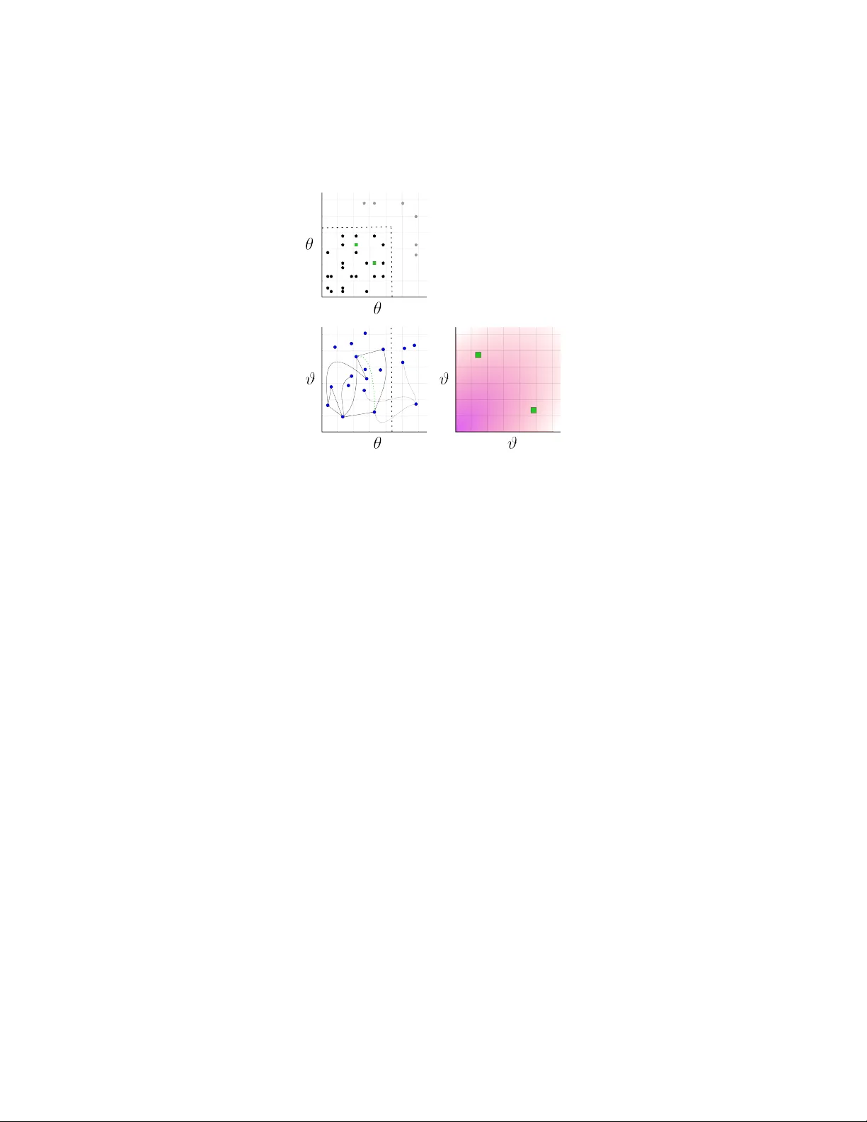
THE CLASS OF RANDOM GRAPHS ARISING FR OM EX CHANGEABLE RANDOM MEASURES VICTOR VEITCH AND DANIEL M. R O Y Abstract. W e in tro duce a class of random graphs that w e argue meets man y of the desiderata one would demand of a mo del to serve as the foundation for a statistical analysis of real-world net works. The class of random graphs is deﬁned by a probabilistic symmetry: inv ariance of the distribution of each graph to an arbitrary relab elings of its vertices. In particular, following Caron and F ox, we interpret a symmetric simple p oint process on R 2 + as the edge set of a random graph, and formalize the probabilistic symmetry as joint exchangeabilit y of the point pro cess. W e give a representation theorem for the class of random graphs satisfying this symmetry via a straightforw ard sp ecialization of Kallenberg’s representation theorem for jointly exchangeable random measures on R 2 + . The distribution of every such random graph is characterized by three (p otentially random) components: a nonnegativ e real I ∈ R + , an in tegrable function S : R + → R + , and a symmetric measurable function W : R 2 + → [0 , 1] that satisﬁes several weak integrabilit y conditions. W e call the triple ( I , S, W ) a graphex, in analogy to graphons, which characterize the (dense) exchangeable graphs on N . Indeed, the mo del we introduce here contains the exchangeable graphs as a special case, as well as the "sparse exchangeable" mo del of Caron and F ox. W e study the structure of these random graphs, and show that they can give rise to interesting structure, including sparse graph sequences. W e give explicit equations for exp ectations of certain graph statistics, as well as the limiting degree distribution. W e also show that certain families of graphexes give rise to random graphs that, asymptotically , contain an arbitrarily large fraction of the vertices in a single connected comp onent. Contents 1. In tro duction 1 2. Bac kground 6 3. Examples 13 4. Representation Theorem for Random Graphs represented b y Exc hangeable Symmetric Simple Poin t Pro cesses 16 5. Exp ected Num b er of Edges and V ertices 22 6. Degree Distribution in the Asymptotic Limit 26 7. Connectivit y for Sep arable KEGs 40 8. Discussion 48 A c knowledgemen ts 50 References 50 1. Intr oduction Random graph mo dels are a key to ol for understanding the structure of real-world net works, esp ecially through data. In particular, a random graph mo del can serve as the foundation for a statistical analysis: observed link structure is mo deled as a realization from the random graph mo del, whose parameters are in some unknown 1 2 V. VEITCH AND D. M. ROY conﬁguration. The goal is to then infer the conﬁguration of the parameters, and in doing so, understand prop erties of the netw ork that gav e rise to the observed link structure. The qualit y of the inferences w e can make dep ends in part on the ﬁdelit y of the mo del, but building realistic mo dels of net w orks is challenging: the mo dels must b e simple enough to b e tractable, yet ﬂexible enough to accurately represent a wide range of phenomena. In the setting of densely connected netw orks, the well-kno wn exc hangeable graph model provides a tractable yet general framework. Ho wev er, the v ast ma jority of real-world netw orks are sparsely connected—t w o no des chosen at random are very unlikely to b e directly connected by a link. A ccordingly , for some conﬁguration of their parameters, realistic random graph mo dels for net w orks m ust b e sparse, exhibiting only a v anishing fraction of all p ossible edges as they b ecome large. A t the same time, the link struc ture of real-world netw orks is rich: e.g., in so cial netw orks, phenomena such as homophily (informally , friends of friends are more likely to b e friends), “small-w orld” connectivity (tw o randomly chosen individuals are likely to b e connected by a short path of friendship), and p ow er law degree distributions (the num ber of friends an individual may hav e v aries across man y orders of magnitude) are common [ New09 ; Dur06 ]. It is a remark able gap in mo dern statistical practice that there is no general framew ork for the statistical analysis of real-world netw orks. There is no shortage of prop osals for random graph mo dels of real-world netw orks; ho w ever, these mo dels tend to b e ad hoc, exhibiting certain prop erties of real-world net works by design, but b ehaving pathologically in other asp ects. It is diﬃcult to assess the statistical applicability of such mo dels. One approac h to identifying large but tractable families of random graphs is to consider the family of all random graphs satisfying a small n um b er of natural assumptions. In this pap er, we deﬁne a class of random graph mo dels in terms of a single inv ariance principle: that the distribution of a graph should b e inv ariant to an arbitrary relab eling of its v ertices. F rom this assumption, w e derive and study a general class of random graphs suitable for mo deling netw ork structures. W e show that these random graphs admit a simple, tractable sp eciﬁcation and give rise to complex structures of the kinds observed in real w orld netw orks. Moreo v er, our deriv ation is closely analogous to an approach that has b een used to deﬁne broadly useful statistical mo dels in other settings. F or instance, the classical i.i.d. setting and the graphon setting for densely connected netw orks are b oth deriv ed from analogous inv ariance assumptions [ OR15 ]. Indeed, we show that the exchangeable graph mo dels are a sp ecial case of the mo dels we derive here. These observ ations suggest that the mo dels w e identify in this pap er may b e broadly useful for the statistical analysis of real-world netw orks. T o explain our approach we b egin by reviewing a closely related approach used to deﬁne mo dels for the statistical analysis of densely connected netw orks. In this setting, netw orks are mo deled as random graphs represen ted by their adjacency matrices; an observed n × n adjacency matrix is mode led as the leading size- n principal submatrix of some inﬁnite array of random v ariables. The inﬁnite structure automatically pro vides consistent mo dels for datasets of diﬀerent size. The foundational structural assumption by which the dense graph framework is deﬁned is a probabilistic symmetry: joint exchange ability of the inﬁnite arr ay . This is the requirement that the distribution of the inﬁnite array is inv ariant under joint KALLENBERG EXCHANGEABLE GRAPHS 3 p erm utations of the indices of the arra y; intuitiv ely , this means that the lab eling of the vertices of a graph do es not carry information ab out its structure. The statistical framew ork can b e derived using the Aldous–Ho ov er representation theorem for join tly exchangeable arra ys. Sp ecialized to the case of inﬁnite adjacency matrices, this theorem asserts that the adjacency matrix of a random graph on N is join tly exchangeable iﬀ its distribution can b e written as a mixture ov er a certain privileged family of distributions (namely , the ergo dic measures). Each member of this family is sp eciﬁed in terms of a symmetric, measurable function W : [0 , 1] 2 → [0 , 1] , now known as a gr aphon . It follows that the space of probability distributions on n × n observ ations of a densely connected netw orks can b e parameterized by the space of graphons. A particular consequence of the theorem is that the exp ected n umber of links among ev ery n individuals is  n 2  k W k 1 ; i.e., the graph is either empt y or dense. As stated plainly in [ OR15 ], these mo dels are thus missp eciﬁed as statistical mo dels for real-world netw orks. The deriv ation of the dense graph framework is a particular instance of a general recip e for constructing statistical mo dels: a probabilistic symmetry is assumed on some inﬁnite random structure and an asso ciated represen tation theorem charac- terizes the ergo dic measures, forming the foundation of a framework for statistical analysis. The ﬁrst main contribution of the present pap er is the analogous represen- tation theorem for the sparse (and dense) graph setting, whic h we arrive at by a straigh tforw ard adaptation of a result of Kallenberg [ Kal90 ; Kal05 ]. Our inspiration comes from recent pap er of Caron and F o x [ CF14 ] that exploits a connection b et w een random measures and random graphs to exhibit a class of sparse random graphs. In their pap er, they observ e that their random graphs satisfy a natural analogue of joint exc hangeability when considered as a p oint pro cess and make use of an asso ciated represen tation theorem to study the mo del. The present pap er reverses this chain of reasoning, b eginning with the symmetry on p oint pro cesses and elucidating the full family of random graphs that arise from the asso ciated representation theorem. In the graph context, join t exchangeabilit y of p oint pro cesses retains the interpretation that the lab els of vertices carry no information ab out the structure of the graph. F ollo wing Caron and F ox, we represent random graphs as an inﬁnite simple p oint pro cesses on R 2 + with ﬁnite random graphs given by truncating the supp ort of the p oin t pro cess to a ﬁnite set (see Fig. 3 ). The representation theorem asso ciated to join t exchangeabilit y of p oin t pro cesses is kno wn b y the work of Kallenberg [ Kal90 ; Kal05 ]. W e arrive at our represen tation theorem by a straightforw ard translation of this result into the random graph setting. The random graphs pic k ed out b y our represen tation theorem ha v e three p ossible comp onen ts: isolated edges, inﬁnite stars, and a ﬁnal piece that provides the interesting graph structure. The basic ob ject for the distributions of these random graphs is a triple ( I , S, W ) where I ∈ R + , S : R + → R + is integrable, and W : R 2 + → [0 , 1] is a symmetric measurable function satisfying certain weak integrabilit y conditions. (See Theorem 4.9 ; W in tegrable is suﬃcient but not necessary .) W e call the triple a gr aphex . In this paper we fo cus on random graphs without isolated edges or inﬁnite stars, and so we take I = S = 0 ; when there is no risk of confusion, we will use the term gr aphex to refer to the function W alone with the understanding that the triple is then of the form (0 , 0 , W ) . The distribution of every suc h random graph, which we call a Kallen b erg exchangeable graph, is characterized b y some (p ossibly random) graphex. 4 V. VEITCH AND D. M. ROY Graphexes are the analogues of graphons and the space of distributions on (sparse) graphs can b e parameterized by the space of graphexes. It remains to explain the construction of the random graph asso ciated with a graphex. Let θ = R + b e the space of lab els of the graph, ϑ = R + b e the space of laten t parameters, and Π b e a unit rate P oisson pro cess on θ × ϑ . Intuitiv ely , the random graph is given by indep endently randomly including each pair of p oints in Π as an edge of graph with a probability determined by the graphex W . A p oin t of the P oisson pro cess is included as a vertex of the graph if and only if it participates in at least one edge. The construction of the random graph is explained in Fig. 1 . F ormally , treating the collection of edges { ( θ i , θ j ) } as the basic random ob ject of in terest the generativ e mo del giv en W and Π is: ( θ i , θ j ) | W, Π ind ∼ Bernoulli( W ( ϑ i , ϑ j )) . (1.1) Finite size graphs are given by restricting to only edges ( θ i , θ j ) suc h that θ i , θ j < ν and including v ertices only if they participate in at least one such edge. These distributions are consistent for datasets of diﬀeren t sizes and admit sparse graphs, allo wing for the realistic mo deling of physical net works. Moreo ver, in a sense we mak e precise in Section 3.1 , the exchangeable graphs derived from the Aldous– Ho o ver theory are contained as a subfamily of the Kallen b erg exchangeable graphs, and corresp ond those graphs generated by graphexes of the form (0 , 0 , W ) where W is compactly supp orted, and therefore equal to the dilation of some graphon. Thus the KEG framework is a generalization of the exchangeable graph framework to the sparse graph regime. Let G ν b e the random graph giv en b y truncating the lab el space θ to [0 , ν ] (see Fig. 1 ); we call the random graph mo del ( G ν ) ν ∈ R + the Kal lenb er g exchange able gr aph (KEG) asso ciated with W . The bulk of the present pap er is dev oted to deriving prop erties of these graphs in terms of the graphex W . F or simplicity of presen tation we ignore self edges here, giving full statemen ts in the b o dy of the pap er. Let µ W ( x ) = ´ R + W ( x, y )d x . (1) Giv en a p oint ( θ , ϑ ) in the latent Poisson pro cess, the degree of the v ertex lab eled θ is Poisson distributed with mean ν µ W ( ϑ ) . (2) The exp ected num ber of edges e ν = | e ( G ν ) | is E [ e ν ] = 1 2 ν 2 ¨ R 2 + W ( x, y )d x d y . (1.2) (3) The exp ected num ber of vertices v ν = | v ( G ν ) | is E [ v ν ] = ν ˆ R + (1 − e − ν µ W ( x ) )d x. (1.3) (4) Sub ject to some technical constraints, the scaling limit of the asymptotic degree distribution has an explicit expression in terms of W . Let k ν b e some non-decreas ing function of ν and let D ν b e the degree of a randomly selected vertex of G ν , then P ( D ν ≥ k ν | G ν ) p − → lim ν →∞ P ∞ k = k ν ν k k ! ´ µ W ( x ) k e − ν µ W ( x ) d x ´ R + (1 − e − ν µ W ( x ) )d x . (1.4) This result establishes that the random graph construction in this pap er can give rise to sparse graphs. KALLENBERG EXCHANGEABLE GRAPHS 5 Figure 1. (Kallen b erg exc hangeable graph) Random graphs arising from exchangeable random measures are c haracterized b y three (p otentially random) comp onents: a non-negativ e real I ∈ R + , an integrable function S : R + → R + , and a symmetric measurable function W : R 2 + → [0 , 1] satisfying some w eak in tegrability conditions. W e call the triple ( I , S, W ) a graphex. The most interesting structure arises from W . A particular W is illustrated by the magenta heatmap (low er right). Giv en W , an inﬁnite random graph with a vertex set in θ is generated in this mo del according to: 1. Sample a (latent) unit rate Poisson pro cess Π on θ × ϑ . 2. F or each pair of p oints ( θ i , ϑ i ) , ( θ j , ϑ j ) ∈ Π include edge ( θ i , θ j ) with probability W ( ϑ i , ϑ j ) . 3. Include θ i as a vertex whenever θ i participates in at least one edge. Finite subgraphs are given by restricting the space θ to b e less than some ﬁnite v alue. The low er left panel of the ﬁgure shows a realization of a latent Poisson pro cess with a realization of the edge structure sup erimp osed. A ﬁnite subgraph (black edges) is given by taking only p oints with θ < 4 . 2 . The edge (3 . 2 , 2 . 1) (green, dotted squares) is included with probabilit y W (1 . 1 , 4 . 7) = W (4 . 7 , 1 . 1) ; this is sho wn in the middle panel. Edges that include a point of Π with θ > 4 . 2 (grey , transparent) are not included in the subgraph. V ertices, such as 2 . 7 , that participate only in edges with a terminus that has θ > 4 . 2 are not included in the subgraph. The upp er left panel sho ws the pictured graph as a realization of a random measure on θ × θ space. 6 V. VEITCH AND D. M. ROY (5) Certain choices of W admit highly connected graphs. Supp ose W ( x, y ) = f ( x ) f ( y ) , let C 1 ( G ν ) b e the largest connected comp onent of G ν , and let  > 0 , then lim ν →∞ P ( | C 1 ( G ν ) | > (1 −  ) | v ( G ν ) | ) = 1 . (1.5) This means that the sparse structure can arise in an interesting w ay: it is not simply a consequence of having a collection of disjoint dense graphs. W e b egin by giving background on random graph mo deling and the use of probabilistic symme try in Section 2 . In Section 3 , w e giv e a num b er of illustrative examples of Kallenberg exchangeable graphs to make the construction concrete. In Section 4 , we establish the represen tation theorem and giv e a formal characterization of the mo dels we derive. In Section 5 , we derive the ﬁrst moments of several graph statistics of G ν using p oint pro cess tec hniques, allowing self edges. An expression for asymptotic degree distribution of these graphs in terms of the graphex is derived in Section 6 . Finally , in Section 7 , we study the structure of the Kallen b erg exchangeable graphs generated by graphexes of the form W ( x, y ) = f ( x ) f ( y )1[ x 6 = y ] with the goal of establishing the asymptotic connectivity structure. Sev eral other in teresting features of these random graphs are uncov ered in the course of establishing this result. In particular, we show that degree p ow er la w distributions and “small-world” phenomena arise naturally in this framework. 2. Ba ck gr ound In order to relate the Kallenberg exc hangeable graph mo del to a diverse range of existing random graph mo dels, it will b e useful to hav e a general deﬁnition for the term ‘random graph mo del’. In this pap er, a random graph mo del is an indexed family of graph-v alued random v ariables G s,φ , where s sp eciﬁes the “size” of the graph and takes v alues in a totally ordered set S , and where φ ∈ Φ determines some distributional prop erties (and so could play the role of a parameter in a statistical mo del). W e will write µ s,φ for the distribution of G s,φ . 1 Our deﬁnition is delib erately v ague ab out the meaning of ‘graph-v alued’ as diﬀerent mo dels will naturally b e describ ed in terms of diﬀerent concrete spaces. F or example, the well-kno wn Erdős–Rényi–Gilbert mo del is the family of simple random graphs G n,p on n ∈ N v ertices, where each edge appears indep endently with probability p ∈ [0 , 1] . Concretely , w e can think of G n,p as a random n × n adjacency matrix, or equiv alen tly , as a symmetric n × n arra y of 0 / 1 -v alued (i.e., binary) random v ariables whose diagonal is zero. In a statistical setting, we might mo del the netw ork of friendships among n individuals as a realization of G n,p for some unknown p . In this case, the goal of statistical analysis would b e to make inferences ab out the parameter p giv en some particular observed dataset in the form of an adjacency matrix. The Erdős–Rén yi–Gilb ert mo del can b e seen as sp ecial case of the more general random graph model that arises from the graphon theory or from the Aldous– Ho o ver represen tation theorem. In this case, the size again determines the num b er of v ertices, but the parameter is a graphon, i.e., a symmetric, measurable function W : [0 , 1] 2 → [0 , 1] . (The Erdős–Rényi–Gilbert mo del corresp onds with constant graphons W ( x, y ) = p for some p ∈ [0 , 1] .) This class of random graphs are known 1 In a statistical setting, the family of distributions µ s,φ would b e the natural structure to call a model. Here we adopt the language of graph theorists. KALLENBERG EXCHANGEABLE GRAPHS 7 as the exchange able gr aphs , although we will sometimes refer to them as the (dense) exc hangeable graphs to distinguish them from the Kallenberg exchangeable graphs. In the exchangeable graph mo del, the size parameter is the num b er of vertices. This is the typical approach to indexing random graph mo dels. In contrast, the size parameter of a Kallenberg exchangeable graph mo del is a non-negative real ν that is prop ortional to the square ro ot of the exp e cte d num b er of e dges . 2.1. Desiderata for random graph mo dels. F or the purp ose of mo deling real- w orld netw orks, one of the key prop erties of a random graph model is the relationship b et ween the num ber of edges and vertices. Consider a random graph mo del G s,φ , ﬁx a parameter φ , and let s n ↑ ∞ b e some diverging sequence of sizes. F or a graph G , let | e ( G ) | and | v ( G ) | denote the n umber of edges and vertices, resp ectively . T o a v oid pathologies, we will assume that | v ( G ) | → ∞ as n → ∞ . Then the sequence ( G s n ,φ ) is sp arse or not dense if, with probability one, p | e ( G ) | | v ( G ) | → 0 as n → ∞ . (2.1) This condition states that, asymptotically , graphs with v v ertices hav e o ( v 2 ) edges. More generally , it is interesting to iden tify whether there is a (p otentially random) exp onen t k suc h that, asymptotically , there are Θ( v k ) edges. F or statistical applications, it is desirable to imp ose a desideratum in addition to sparsit y . The protot ypical statistical netw ork analysis has the following structure: an observed netw ork g s is mo deled as a realization of a random graph G s,φ for some size s and for some unkno wn parameter φ ; the goal is to infer the parameter φ . In some random graph mo dels, the sequence G s 1 ,φ , G s 2 ,φ , . . . of graphs is a mo del of the dynamics b y which a netw ork grows and evolv es. In the statistical problems motiv ating this pap er, how ev er, the size parameter s is akin to sample size in the sense that collecting more data corresp onds to c ho osing larger v alues of s . It is therefore natural to demand that the distributions asso ciated with diﬀerent sizes are “consistent” with one another in the sense that moving from G s,φ to G t,φ , for t > s , can b e understo o d as collecting additional data. One w ay to formalize this notion of consistency is to demand that the distributions of the random graphs G s,φ b e pr oje ctive . Pro jectivity is deﬁned in terms of a pro jectiv e system, i.e., a family of measurable maps ( f s,t ; s ≤ t ∈ S ) where f s,t maps graphs of size t to graphs of size s ≤ t , f s,s is the identit y , and f r,t = f r,s ◦ f s,t for all r ≤ s ≤ t . A random graph mo del is pr oje ctive if, for some pro jective system ( f s,t ; s ≤ t ∈ S ) , it holds that G s,φ d = f s,t ( G t,φ ) for every s < t ∈ S and parameter φ . In tuitively , this is simply the requiremen t that a data set of size t can be understo o d as a data set of size s < t augmen ted with some additional observ ations. Indeed, if a random graph mo del ( G s,φ ) is pro jective with resp ect to a pro jective system ( f s,t ; s ≤ t ∈ S ) , then it is p ossible to construct the random v ariables G s,φ in su c h a wa y that the identit y G s,φ = f s,t ( G t,φ ) holds almost surely , and not only in distribution. In view of this, the connection with the idea of s as sample size is clear. The graphs G s j ,φ for an increasing sequence s 1 , s 2 , . . . of sizes are nested. Both the (dense) exc hangeable graph mo del and the Kallenberg exc hangeable graph mo del are pro jectiv e. (See Figs. 1 and 2 for illustrations). The (dens) exc hangeable graph mo del is pro jective with resp ect to the maps f m,n that take an n × n adjacency matrix to its principal leading m × m submatrix. In other words, 8 V. VEITCH AND D. M. ROY dropping the last n − m ro ws and columns from G n,W pro duces an arra y with the same distribution as G m,W . The Kallenb erg exchangeable graph mo del is pro jectiv e with resp ect to the maps f s,t that take a measure on [0 , t ] 2 to its restriction on [0 , s ] 2 . In other words, G s,W d = G t,W ( · ∩ [0 , s ] 2 ) for all s, t ∈ R + . The pro jectivity of the KEG mo del sets it apart from random graph mo dels that ac hiev e sparsit y b y p ercolating dense random graph mo dels such as the exchangeable graph model, i.e., a sparse graph mo del is produced by randomly deleting each edge in a dense graph mo del indep endently with a probability that grows with the n umber of vertices. Examples of such mo dels ab ound [ BJR07 ; BR07 ; BCCZ14a ; BCCZ14b ], and in some cases consisten t estimators hav e b een developed [ WO13 ; BCCG15 ; BCS15 ]. Eac h of these random graph mo dels is parametrized by a size n that determines the num ber of vertices, and, for every size n , these random graph mo dels are also jointly exchangeable. It then follows from the Aldous–Ho ov er and graphon theory , as well as the fact that they are not dense, that these random graph mo dels are not pro jective. While dropping pro jectivity allow ed for sparse random graph mo dels, the lack of pro jectivit y complicates the statistical applicabilit y of these mo dels. A t the very least, the interpretation of the aforemen tioned consistency results is not straigh tfor- w ard. Indeed, these mo dels are usually understo o d to generate the size n graphs indep enden tly of each other. Even an adaptation of these mo dels designed to imp ose some consistency b etw een datasets of diﬀerent size seems inappropriate for mo deling data observ ation as, for instance, every time a new vertex is observ ed some fraction of the edges already in the graph will b e randomly deleted. 2.2. Mo dels from symmetries. Up until this p oint, we ha ve fo cused on very general desiderata for random graph mo dels. Merely requiring sparsity and pro jec- tivit y , how ev er, do es not alone lead to a tractable class of mo dels. Indeed, without an y restrictions on the mo del, data will con vey no information as to the pro cess that gav e rise to it. T o enable statistical inference, it is necessary to mak e some structural assumptions on the parametrization of the random graph mo del. A t the same time, w e w an t a ﬂexible mo del to serve as the foundation of a broadly applicable framew ork for the statistical analysis of netw ork data, and so we wan t to imp ose as few assumptions as p ossible. A general approach tow ards identifying large tractable families of distributions is to consider the class of all distributions satisfying a particular inv ariance. The structure of such inv ariant classes can b e understo o d in general terms using very general results on ergo dic decompositions, or, in some cases, via explicit c harac- terizations given by so-called representation theorems. Both (dense) exchangeable graphs and KEGs are examples of such families, but to clarify the idea of deﬁning a class of mo dels by an inv ariance principle, we will review a fundamental class of examples: the exchangeable sequences. (The following developmen t ow es muc h to [ OR15 ], where the reader can ﬁnd more details.) Consider the classical setting of statistical inference: a sequence of real-v alued measuremen ts x 1 , . . . , x n are made of a system in some unkno wn conﬁguration, and this sequence is mo deled as a realization from some unknown distribution µ n ∈ M 1 ( R n ) . If, in principle, we could hav e made any n um b er of measurements, then there exists a sequence of distributions µ 1 , µ 2 , . . . that are pro jectiv e with resp ect to the maps f m,n that take length- n sequences to their length- m preﬁxes. It follo ws from general results in probability theory that there exists an inﬁnite sequence KALLENBERG EXCHANGEABLE GRAPHS 9 X 1 , X 2 , . . . of random v ariables suc h that µ n is the distribution of ( X 1 , . . . , X n ) . Therefore, we are mo deling observed length- n sequences ( x 1 , . . . , x n ) as realizations of preﬁxes ( X 1 , . . . , X n ) of the inﬁnite random sequence ( X 1 , X 2 , . . . ) . Let µ b e the unkno wn distribution of the inﬁnite sequence. Without making any further assumptions, it would seem that µ is an unknown elemen t of the space M 1 ( R ∞ ) of all distributions on inﬁnite sequences of real n um b ers. How ev er, a ﬁnite preﬁx of a realization dra wn from an arbitrary elemen t µ ∈ M 1 ( R ∞ ) do es not con v ey any information ab out the generating process µ . Ho w ever, if we assume that the inﬁnite sequence of random v ariables X 1 , X 2 , . . . is exchange able , i.e., ( X 1 , . . . , X n ) d = ( X σ (1) , . . . , X σ ( n ) ) (2.2) for every n ∈ N and every p ermutation σ of [ n ] = { 1 , . . . , n } , then, by de Finetti’s represen tation theorem [ Fin30 ; Fin37 ; HS55 ], the random v ariables X 1 , X 2 , . . . are conditionally i.i.d., i.e., there exists a probability measure P on the space M 1 ( R ) of probabilit y measures on R such that M ∼ P (2.3) X 1 , X 2 , . . . | M iid ∼ M . (2.4) W e can express the distribution µ in terms of P : F or a distribution m on R , let m ∞ b e the distribution of an inﬁnite i.i.d.- m sequence. Then µ ( B ) = ˆ M 1 ( R ) m ∞ ( B ) P (d m ) , for measurable B ⊆ R ∞ . (2.5) The distribution µ is uniquely determined by P , and vice versa. F rom Eq. ( 2.5 ), w e can see that the space of distributions of exchangeable sequences is a conv ex set. It is kno wn that ev ery such distribution can b e written as a unique m ixture of the inﬁnite pro duct measures of the form m ∞ , whic h are the extreme p oints. These extreme p oin ts are precisely the er go dic me asur es . The statistical utility of exchangeabilit y is obvious: it follo ws from the disintegra- tion theorem [ Kal01 , Thm. 4.4] and the law of large num b ers that M ( A ) = lim n →∞ 1 n n X j =1 1( X j ∈ A ) a.s. (2.6) On the other hand, even an inﬁnite realization ( x 1 , x 2 , . . . ) giv es no information ab out P . F or this reason, in a statistical setting, in addition to assuming that ν is an element in the space of distributions of exc hangeable sequences, we assume that ν is ergo dic, i.e., ν is an unknown element in the space of distributions of i.i.d. sequences. Since ev ery ν has the form m ∞ for some probability measure m on R , it follows that the natural parameter space is the space M 1 ( R ) , and our mo del is µ n,φ = φ n . The statistical utility of exc hangeabilit y is not merely a matter of theoretical con venience; the v ast ma jorit y of statistical practice falls under the remit of this framew ork. Inference of the kind taught in introductory statistics courses is recov ered b y restricting P to ha ve supp ort only on families of mo dels with ﬁnite dimensional parameterizations, e.g., the normal distributions. The case where P has supp ort on distributions without ﬁnite dimensional parameterizations are so called non- parametric mo dels, of which there are many practical examples. 10 V. VEITCH AND D. M. ROY It is worth emphasizing that although de Finetti’s representation theorem is often c haracterized as a justiﬁcation for the use of indep endence in Bay esian mo deling, for our purp oses the deep er p oin t is that assuming a probabilistic symmetry characterizes the primitiv e of random sequence mo dels ( M , a probability distribution on R ) and giv es a simple generative recip e for the data in terms of thi s primitive. It is this later p erspective that is paralleled in the deriv ation of the KEG mo del. 2.3. Mo dels for graphs from symmetries. W e hav e seen how the assumption that an idealized inﬁnite sequence of observ ations is exchangeable leads to a consid- erable simpliﬁcation of the space of distributions under consideration. Moreo v er, it is clear that ﬁnite samples can b e used to make inferences ab out the generating pro cess. W e no w turn to related results for netw orks. In particular, we derive the traditional exchangeable graph mo del from exchangeabilit y and then connect it to the Kallenberg exchangeable graph mo del. Consider a partial observ ation of a netw ork: an array of measurements x i,j , for 1 ≤ i, j ≤ n , are made betw een n en tities n um b ered from 1 to n . W e write x i,j = 1 if a link exists b etw een i and j , and write x i,j = 0 otherwise. W e will assume the relationship is symmetric, i.e., x i,j = x j,i and that no entit y links to itself, i.e., x i,i = 0 . In other w ords, our data is a simple graph ov er n v ertices, and we can mo del it as a realization from some distribution µ n ∈ M 1 ( { 0 , 1 } n × n ) concen trating on symmetric arra ys with zeros along the diagonal. If, in principle, w e could hav e collected data on any n um b er of entities, then there exists a sequence of distributions µ 1 , µ 2 , . . . that are pro jectiv e with resp ect to the maps f m,n that tak e n × n arra ys to their leading m × m subarra ys. Again, from general results in probabilit y theory , there exists an inﬁnite array of random v ariables X i,j , for i, j ∈ N , suc h that µ n is the distribution of ( X i,j ; i, j ≤ n ) . Therefore, we mo del observed n × n adjacency matrices ( x 1 , . . . , x n ) as realizations of preﬁxes ( X i,j ; i, j ≤ n ) of the inﬁnite adjacency matrix ( X i,j ; i, j ∈ N ) . Let µ b e the distribution of the inﬁnite arra y matrix. Let us now consider probabilistic symmetries on this inﬁnite idealized netw ork observ ation. The class of exchangeable sequences has a literal—if naïve—coun terpart in the graph setting: the class of edge-exchangeable graphs. The assumption that the edges are exchangeable is the assumption that ( X i,j ; i, j ≤ n ) d = ( X σ ( i,j ) ; i, j ≤ n ) , (2.7) for every n ∈ N and every permutation σ of [ n ] × [ n ] that is symmetric, i.e., σ ( i, j ) = ( i 0 , j 0 ) if and only if σ ( j, i ) = ( j 0 , i 0 ) . This assumption is to o severe, ho wev er, b ecause it is simply exchangeabilit y of a sequence in disguise. T o see this, let N 2 b e the set of pairs ( i, j ) ∈ N 2 suc h that i < j let ι : N → N 2 b e an arbitrary bijection, and deﬁne Y n = X ι ( n ) . Then Eq. ( 2.7 ) implies that the sequence of random v ariables Y 1 , Y 2 , . . . are exchangeable and so they are conditionally i.i.d. But then the edges X ι ( n ) , for n ∈ N , are also conditionally i.i.d. Therefore, there exists a random v ariable p in [0 , 1] suc h that, conditioned on p , the edges X i,j are i.i.d. and each edge app ears with probability p . This is none other than the Erdős–Rényi–Gilbert mo del with a random edge probability . The class of ergo dic measures in this case is precisely the Erdős–Rényi–Gilbert mo del. The natural analogue of exc hangeability in the graph setting is to assume that the lab els of the vertices are exchangeable. Informally , this is the assumption that the v ertex lab els carry no information. Giv en that w e are represen ting an observ ed KALLENBERG EXCHANGEABLE GRAPHS 11 adjacency matrix as a preﬁx of an idealized inﬁnite symmetric binary array , vertex- exc hangeability is formalized as the requirement that distribution of the array is in v ariant under simultaneous p ermutation of its rows and columns. More carefully , an array of random v ariables X i,j is jointly exchange able when ( X i,j ; i, j ≤ n ) d = ( X σ ( i ) ,σ ( j ) ; i, j ≤ n ) (2.8) for every n ∈ N and every p ermutation σ of [ n ] . A characterization of inﬁnite jointly exc hangeable adjacency matrices can b e easily derived from the Aldous–Hov er represen tation theorem for general jointly exchangeable arrays [ Ald81 ; Ho o79 ]. In particular, ev ery ergo dic measures is characterized b y a symmetric measurable function W : [0 , 1] 2 → [0 , 1] , whose diagonal is zero. This same ob ject w as later redisco vered indep endently by graph theorists as the limit ob ject in a theory of limits of dense graphs [ LS06 ; LS07 ; Lov13 ]. In this context it w as named a graphon, whic h is the nomenclature we use here. The relationship b etw een the graphon as the deﬁning ob ject for distributions of jointly exchangeable arrays and as the limit ob ject of dense graph theory is explained b y [ DJ08 ]. More concretely , the generative mo del for vertex-exc hangeable graphs is (see Fig. 2 ) W ∼ µ (2.9) { U i } iid ∼ Uni[0 , 1] (2.10) ( X ij ) | W, U i , U j ind ∼ Bernoulli( W ( U i , U j )) , (2.11) where µ is a measure on the space of symmetric functions from the unit square to the unit in terv al with zero diagonal. The fact that pro jective and jointly exchangeable adjacency matrices cannot b e sparse is a simple consequence of this generative mo del and the law of large num bers. In particular, any nondiagonal en try is one with probabilit y k W k 1 . This framework is the exchangeable graph mo del, whose nomenclature is now self explanatory . Comparing the generativ e mo del for the exc hangeable graph mo del with the KEG generative mo del (see Fig. 1 ) makes it clear that the distinction that allows for more general graphs in the KEG setting is that the latent v ariables asso ciated with each vertex are not indep endent, and the sizes of the graphs are random. It is p ossible to construct a sparse and pro jectiv e random graph mo del if w e drop the requirement that the arrays of each size n ∈ N b e exchangeable. F or example, the preferential attac hmen t mo del of [ BA99 ] can b e understo o d in these terms, although historically it w as developed indep endently of these concerns for the sp ecial purp ose of giving a mechanism of graph gr owth that leads to p o w er law b eha vior in the degree distribution. A d ho c mo dels of this kind tend to fail to capture certain k ey elements of real-world netw ork structure. F or instance, as shown by [ BBCS14 ], the limiting lo cal structure of preferen tial attachmen t graphs is a tree, and so these net w orks would b e pathological mo dels of so cial netw orks, which exhibit homophily . 2.4. Random graphs as random measures. The key ingredien t for generalizing the exchangeable graph mo del is a corresp ondence betw een random graphs and symmetric simple p oint pro cesses due to Caron and F ox [ CF14 ] (see Fig. 3 ). Again, restricting ourselves to simple graphs for simplicity of presen tation, the edge set of a random graph is a random ﬁnite or countable collection of tuples ( x, y ) ∈ R 2 + , and the vertex set is the set of those real num bers x suc h that x participates in at least 12 V. VEITCH AND D. M. ROY Figure 2. Graphon random graph mo del. In the jointly ex- c hangeable array setting a random graph mo del is character- ized by a (p otentially random) symmetric measurable function W : [0 , 1] 2 → [0 , 1] called a graphon. An example graphon is de- picted as a magenta heatmap (low er right). Conditional on W , a random graph of size n is generated by indep endently assigning to eac h v ertex k ∈ { 1 , . . . , n } a laten t random v ariable U k ∼ Uni (0 , 1) (v alues along vertical axis) and including each edge ( k , l ) indep en- den tly with probability W ( U k , U l ) . F or example, edge (3 , 5) (green, dotted) is present with probabilit y W (0 . 72 , 0 . 9) ; the green b oxes in the right square represent the v alues of ( u 3 , u 5 ) and ( u 5 , u 3 ) . The upp er left panel shows the graph realization as an adjacency matrix. one edge. Concretely , the random graph is represented by a simple point pro cess G on R 2 + con taining a p oin t ( x, y ) iﬀ there is an edge ( x, y ) in the random graph. It will b e mathematically conv enien t to represent simple p oin t pro cesses b y simple random measures, i.e., purely atomic random measures whose atoms all ha ve mass one. In this case, each atom in the simple random measure represents a p oint of the p oin t pro cess. Having made this c hoice, the idealized inﬁnite observ ation in this setting is the inﬁnite p oint pro cess G , and ﬁnite observ ations are the restrictions G t = G ( · ∩ [0 , t ] 2 ) , for t ∈ R + , of the inﬁnite p oint pro cess G to the b ounded square subsets [0 , t ] 2 ⊂ R 2 + con taining the origin. The distribution of these restrictions of G are automatically pro jectiv e with resp ect to the maps f s,t that tak es a measure on [0 , t ] 2 to its restriction on [0 , s ] 2 . In contrast to the exchangeable graph mo del, the KEG mo del has a contin uously indexed size parameter and the n umber of v ertices in each ﬁnite restriction G t is itself a random quantit y . It is imp ortant to note that the graph corresp onding to the restriction G s to [0 , s ] 2 has as its vertex set only those vertices x ∈ [0 , s ] that app ear in some edge ( x, y ) where y ∈ [0 , s ] . In particular, there will, in general, b e vertices in [0 , s ] that app ear for the ﬁrst time in a restriction [0 , t ] , for t > s . This is an essential prop erty of this represen tation, and is the wa y that the seeming equiv alence b etw een exchangeabilit y and density can b e relaxed. The point lab eled 2.7 in Fig. 1 provides a concrete example of this phenomena. KALLENBERG EXCHANGEABLE GRAPHS 13 Figure 3. Random graphs as p oint pro cesses. Random p oint pro cesses on R 2 + corresp ond to inﬁnite random graphs, with ﬁnite subgraphs giv en b y restricting the p oint pro cess to a ﬁnite square. P oints of the pro cess corresp ond to graph edges and the v ertex structure is deduced from the edge structure. Pictured is a real- ization of a p oin t pro cess and the realization of the random graph that corresp onds to truncating at θ = 5 . As observ ed by Caron and F o x, when random graphs are represented as p oint pro cesses, vertex-exc hangeabilit y corresp onds to joint exchangeabilit y for r andom me asur es . F ormally , a random measure ξ on R 2 + is jointly exchange able when ξ d = ξ ◦ ( f ⊗ f ) − 1 (2.12) for every measure preserving transformation f : R + → R + , where ⊗ is the tensor pro duct. This probabilistic symmetry was in troduced by Aldous, who also con- jectured a concrete representation theorem [ Ald85 , Conj. 15.15], later established rigorously by Kallenberg [ Kal90 ; Kal05 ]. W e will refer to the representation theorem as the Kallenberg representation theorem. W e now describ e the Kallenberg exchangeable graph mo del plainly: It is the random graph mo del that arises from the symmetry of joint exc hangeabilit y of symmetric simple p oint pro cesses on R 2 + , when these structures are interpreted as the edge sets of random graphs. W e giv e a representation theorem for these structures via a straightforw ard application of Kallenberg’s represen tation theorem in the sp eciﬁc context of symmetric simple p oint pro cesses on R 2 + . F rom this result, w e see that every ergo dic measure is determined by a triple ( I , S, W ) , whic h w e call a graphex. F rom a statistical standp oint, the graphexes are the natural parameters, and every random graph is seen to arise via the corresp onding generative pro cess (Fig. 1 ). The KEG mo del is pro jective, exchangeable, and admits sparse graphs, thereb y pro viding a statistical framework for net work analysis that a v oids some of the pitfalls of other random graph mo dels. Both the traditional exchangeable graph mo del and the Caron–F o x mo del are sp ecial cases, and so the KEG mo del can b e seen as a generalization and uniﬁcation of these mo dels. 3. Examples The aim of this section is to w ork through the details of several informativ e examples to build intuition for the structure of the Kallenberg exchangeable graph mo dels we consider here. W e fo cus on those graphexes where I = S = 0 , and so we will refer to W as the graphex without an y risk of confusion. W e are particularly in terested in the sparsity of these graph mo dels. Theorem 5.3 establishes that (ignoring self edges) for all random graphs G ν generated by graphex W it holds that E [ e ν ] = 1 2 ν 2 k W k 1 ; i.e., the exp ected num ber of edges scales as ν 2 in all cases. 14 V. VEITCH AND D. M. ROY In tuitiv ely then we exp ect the sparsity of a random graph mo del to b e determined b y E [ v ν ] = ν ´ R + 1 − e − ν µ W ( x ) d x (from Theorem 5.4 , ignoring self edges). This suggests that the slow er µ W ( x ) = ´ R + W ( x, y )d y deca ys the sparser the graph will b e, an intuition that is b orne out by the examples of this section. 3.1. Graphon mo dels. The ab ov e argument suggests that the most densest graphs will corresp ond to those W that are compactly supp orted. Let f W : [0 , 1] 2 → [0 , 1] b e a graphon and consider the graphex given by the dilation W ( x, y ) = ( f W ( x/c, y /c ) x ≤ c, y ≤ c 0 otherwise. (3.1) In this case, p oints ( θ , ϑ ) ∈ Π of the laten t Poisson pro cess will fail to connect to an edge if ϑ > c , and so such p oints they never participate in the graph and can b e discarded. This means that for ﬁnite size graph G ν giv en by restricting θ ≤ ν the relev ant underlying pro cess is the unit rate Poisson pro cess on [0 , ν ] × [0 , c ] . The generativ e mo del for the graph can b e expressed as: N ν ∼ Poi( c ν ) (3.2) { θ i } | N ν iid ∼ Uni[0 , ν ] (3.3) { ϑ i } | N ν iid ∼ Uni[0 , 1] (3.4) ( θ i , θ j ) | f W , ϑ i , ϑ j ind ∼ Bernoulli( f W ( ϑ i , ϑ j )) . (3.5) A little though t shows that this is just a trivial mo diﬁcation of the graphon mo del. Instead of indexing the family of graphs by the num b er of v ertices ( N ) w e now index them by the contin uous parameter ν and hav e P oi ( c ν ) candidate vertices at each stage. The vertices now hav e i.i.d. uniform lab els instead of the integer lab els of the traditional graphon mo del and vertices are only included if they connect to at least one edge. The critical comp onents of the graphon mo del structure are unchanged: the primitive is still the graphon f W : [0 , 1] 2 → [0 , 1] , the conditional indep endence of the edges is the same, the latent v ariables are indep enden t, and these graphs are necessarily asymptotically dense (or empty). This is the sense in whic h the graphon mo del is a sp ecial case of the graphex mo del derived in this pap er. In fact, these are the only dense KEGs arising from (integrable) graphexes: Theorem 5.6 sho ws that G is dense iﬀ the generating (in tegrable) graphex has compact supp ort. 3.2. Slo w Decay. W e next consider a graphex with tails that go to 0 slowly: W ( x, y ) = ( 0 x = y , ( x + 1) − 2 ( y + 1) − 2 otherwise, (3.6) where the condition W ( x, x ) = 0 ∀ x ∈ R + forbids self edges. In this case µ W ( x ) = 1 3 ( x + 1) − 2 and by Theorem 5.4 E [ v ν ] = ν ( √ π p ν / 3 erf ( p ν / 3) + e − ν / 3 − 1) (3.7) ∼ r π 3 ν 3 / 2 , ν → ∞ . (3.8) KALLENBERG EXCHANGEABLE GRAPHS 15 By Theorem 5.5 the num ber of vertices with degree k has exp ectation: E [ N ν,k ] = ν k +1 k ! ( 1 3 ) k ˆ ∞ 1 x − 2 k e − 1 3 ν x − 2 d x (3.9) = ν k +1 k ! ( 1 3 ) k ˆ 1 0 x 2( k − 1) e − 1 3 ν x 2 d x (3.10) = Γ( − 1 2 + k ) − Γ( − 1 2 + k , ν 3 ) 2 √ 3 k ! ν 3 / 2 (3.11) ∼ Γ( − 1 2 + k ) 2 √ 3 k ! ν 3 / 2 , ν → ∞ . (3.12) By Theorem 6.1 it follows that the degree D ν of a uniformly selected vertex of G ν satisﬁes P ( D ν = k | G ν ) p − → Γ( − 1 2 + k ) 2 √ π k ! , ν → ∞ , (3.13) so in particular a randomly selected vertex of G ν will hav e ﬁnite degree ev en in the inﬁnite graph limit. F or large k Γ( − 1 2 + k ) 2 √ π k ! ∼ k − 3 2 , k → ∞ , (3.14) so this is an example of a random graph mo del with p ow er-la w degree distribution. Note that, in the limit, while the degree of a randomly c hosen vertex is ﬁnite almost surely , it is inﬁnite in exp ectation. 3.3. F ast D eca y. Next we consider a graphex with quickly decaying tails. Let W ( x, y ) = ( 0 x = y e − x e − y otherwise. (3.15) Then µ ( x ) = e − x and so by Theorem 5.4 E [ v ν ] = ν ˆ R + 1 − e − ν e − x d x (3.16) = ν ˆ 1 0 1 x (1 − e − ν x )d x (3.17) = ν ( γ + Γ(0 , ν ) + log( ν )) (3.18) ∼ ν log ν, ν → ∞ . (3.19) As exp ected, the rapidly deca ying graphex giv es rise to a graph that is muc h more dense than one from the slowly decaying graphex. By Theorem 5.5 the num ber of vertices with degree k has exp ectation: E [ N ν,k ] = ν k +1 k ! ˆ ∞ 0 e − kx e − ν e − x d x (3.20) = ν k ! (Γ( k ) − Γ( k , ν )) (3.21) ∼ ν k , ν → ∞ . (3.22) 16 V. VEITCH AND D. M. ROY so that for ﬁxed k only a v anishing fraction of the vertices will hav e degree k as ν → ∞ . More precisely , since P ν β k =1 ν k ∼ β ν log ν , ν → ∞ we ha ve b y Theorem 6.1 that for 0 < β < 1 P ( D ν ≤ ν β ) p − → β , ν → ∞ (3.23) where D ν is a random vertex of G ν . 3.4. Caron and F ox. As already alluded to, the family of random graph mo dels considered b y Caron and F o x in [ CF14 ] is a sp ecial case of the one considered here. Indeed, in their pap er they prov e their mo del satisﬁes joint exchangeabilit y when considered as a random measure and use Kallen b erg’s representation theorem to deriv e some mo del prop erties. Nev ertheless, the connection is opaque b ecause their mo del is constructed from pro ducts of completely random measures and they cast their mo del in terms of Lévy pro cess intensities. If the θ × θ measure they had studied had b een a pro duct of completely random measures, that mo del would ha ve corresp onded to a graphex of the form W ( x, y ) = f ( x ) f ( y ) . Instead, they actually consider a measure on θ × θ giv en by using the pro duct of completely random measures as a base measure for a Cox pro cess. This gives rise to a directed m ultigraph which is then transformed into a simple graph b y including edge { θ i , θ j } if and only if there is at least one directed edge b etw een θ i and θ j . A little algebra sho ws this mo del corresp onds to the graphex W ( x, y ) = ( 1 − exp( − g ( x ) g ( y )) x = y 1 − exp( − 2 g ( x ) g ( y )) x 6 = y (3.24) where g ( x ) : R + → R + . Caron and F o x derive this expression in their pap er, and giv e g in terms of the intensit y of the deﬁning Lévy pro cess. 4. Represent a tion Theorem f or Random Graphs represented by Ex changeable Symmetric Simple Point Processes W e no w turn to giving formal statements of our construction and pro ving the represen tation theorem at the heart of the pap er. In fact, this mostly amoun ts to translating Kallen b erg’s representation theorem for jointly exchangeable random measures on R + to the random graph setting. The cen tral ob jects of study here are undirected, un weigh ted graphs whose v ertices are lab eled with v alues in R + . F or a graph G , w e will write v ( G ) and e ( G ) to denote the set of vertices and edges, resp ectively . W e b egin by formalizing the idea of a graph represented by a measure. Deﬁnition 4.1. An adjac ency me asur e is a lo cally ﬁnite symmetric simple measure on R 2 + . The ν -trunc ation of an adjacency measure ξ is the adjacency measure ξ ( · ∩ [0 , ν ] 2 ) obtained by restricting ξ to [0 , ν ] 2 . Deﬁnition 4.2. Let G b e a simple graph, p ossibly with lo ops, whose edge set e ( G ) is a lo cally ﬁnite subset of R 2 + . Then the adjac ency me asur e of G is the adjacency measure P ( x,y ) ∈ e ( G ) δ ( x,y ) . Note that the adjacency measures of a graphs G and G 0 coincide if and only if their edge sets do. In particular, vertices that do not participate in an edge are “forgotten”. W e will b e interested in the smallest graph corresp onding to an KALLENBERG EXCHANGEABLE GRAPHS 17 adjacency measure ξ , whic h is necessarily the graph with the same edge set and no isolated vertices. (See Fig. 3 for an illustration.) Deﬁnition 4.3. Let ξ = P i<κ δ e i b e an adjacency measure, where κ ∈ Z + ∪ {∞} and e 1 , e 2 , . . . is a sequence of distinct elements of R 2 + . Then the simple gr aph asso ciate d with ξ is the graph G whose edge set is { e i : i < κ } and whose vertex set is { x : ∃ i < κ ∃ y ∈ R + e i = ( x, y ) } . R emark 4.4 . This corresp ondence extends to directed weigh ted graphs in an obvious w ay by dropping the requiremen t that the adjacency measure b e symmetric and allo wing the adjacency measure to assign a mass other than one to each of its atoms; i.e., a directed weigh ted adjacency measure is a lo cally ﬁnite purely atomic measure, and so would hav e the form ξ = P ij ω ij δ ( θ i ,θ j ) .  A random adjacency measure is an (a.s. lo cally ﬁnite) symmetric simple p oint pro cess. W e will represent random graphs b y their random adjacency measures, noting that only nonisolated vertices are captured by this representation. Informally , we are interested in those simple random graphs embedded in R + whose distributions are inv arian t to every relab eling of the v ertices of the random graph. W e can formalize this notion of inv ariance in terms of a symmetry of the corresp onding adjacency measure. W e b egin with a deﬁnition of exc hangeability for random measures due to Aldous: Deﬁnition 4.5. A random measure ξ on R 2 + is said to b e jointly exchange able if, for every measure preserving transformation f on R + , we hav e ξ ◦ ( f ⊗ f ) − 1 d = ξ . (4.1) The follo wing result, due to Kallen b erg, c haracterizes the space of exc hangeable measures on R 2 + as well as its extreme p oints: Let Λ denote Leb esgue measure on R + and let Λ D denote Leb esgue measure on the diagonal of R 2 + . Theorem 4.6 (Kallen b erg [ Kal05 ; Kal90 ]) . A r andom me asur e ξ on R 2 + is jointly exchange able iﬀ almost sur ely ξ = X i,j f ( α, ϑ i , ϑ j , ζ { i,j } ) δ θ i ,θ j (4.2) + X j,k ( g ( α, ϑ j , χ j k ) δ θ j ,σ j k + g 0 ( α, ϑ j , χ j k ) δ σ j k ,θ j ) (4.3) + X k ( l ( α, η k ) δ ρ k ,ρ 0 k + l 0 ( α, η k ) δ ρ 0 k ,ρ k ) (4.4) + X j ( h ( α, ϑ j )( δ θ j ⊗ Λ) + h 0 ( α, ϑ j )(Λ ⊗ δ θ j )) + β Λ D + γ Λ 2 , (4.5) for some me asur able function f ≥ 0 on R 4 + , g , g 0 ≥ 0 on R 3 + and h, h 0 , l , l 0 ≥ 0 on R 2 + , some c ol le ction of indep endent uniformly distribute d r andom variables ( ζ { i,j } ) on [0 , 1] , some indep endent unit r ate Poisson pr o c esses { ( θ j , ϑ j ) } and { ( σ ij , χ ij ) } j , for i ∈ N , on R 2 + and { ( ρ j , ρ 0 j , η j ) } on R 3 + , and some indep endent set of r andom variables α , β , γ ≥ 0 . The latter c an b e chosen to b e non-r andom iﬀ ξ is extr eme. The task is to translate this into a statement ab out random graphs, or more sp eciﬁcally , their adjacency measures. Because adjacency measures are purely atomic, all terms with a Leb esgue comp onent (Eq. ( 4.5 )) must hav e measure zero. The 18 V. VEITCH AND D. M. ROY remaining purely atomic terms underlying a jointly exchangeable random measure ha v e the follo wing in terpretation for adjacency measures: (1) P i,j f ( α, ϑ i , ϑ j , ζ { i,j } ) δ θ i ,θ j : this term contributes most of the interesting structure for the random graph models. The random measure ξ will be symmetric and simple if and only if f is a.e. { 0 , 1 } -v alued and symmetric in its second and third arguments, for a.e. ﬁxed ﬁrst and fourth argumen t. (It is clear that this can easily b e strengthened to hold ev erywhere.) This leads to the corresp onde nce illustrated in Fig. 1 . (General f could b e used to mo del directed, weigh ted graphs in an ob vious wa y .) The tuples ( θ i , θ j ) are p ossible edges of the graph and the p oints θ i are candidate vertices. (2) P j,k ( g ( α, ϑ j , χ j k ) δ θ j ,σ j k + g 0 ( α, ϑ j , χ j k ) δ σ j k ,θ j ) : this term contributes stars. T o see this, note that each candidate vertex θ j has an asso ciated Poisson pro cess { σ j k } . The p oints are a.s. distinct: i.e., { θ l } ∩ { σ j k } = ∅ and { σ j k } ∩ { σ lk } for j 6 = l with probabilit y one. This means the candidate v ertices { σ j k } will only ev er participate in edges with θ j , hence the star structure. The random measure ξ will b e a.s. symmetric and simple iﬀ g = g 0 and g is { 0 , 1 } -v alued. (3) P k ( l ( α, η k ) δ ρ k ,ρ 0 k + l 0 ( α, η k ) δ ρ 0 k ,ρ k ) : this term contributes isolated edges. T o see this, note that, with probabilit y one, { ρ k } ∩ { ρ 0 k } = ∅ and these candidate vertices do not coincide with any other candidate vertices (e.g., { ρ k } ∩ { θ l } = ∅ ). This means that if ( ρ i , ρ j ) is an edge of the graph then with probability 1 ( ρ i , x ) will not be an edge for an y x ∈ R + . Again, the random measure ξ will b e a.s. symmetric and simple iﬀ l = l 0 and l is { 0 , 1 } -v alued. The follo wing theorem c haracterizes the space of exchangeable adjacen cy measures as well as its extreme p oints: Theorem 4.7 (Random graph represen tation) . L et ξ b e a r andom adjac ency me a- sur e. Then ξ is jointly exchange able iﬀ almost sur ely ξ = X i,j 1[ W ( α, ϑ i , ϑ j ) ≤ ζ { i,j } ] δ θ i ,θ j (4.6) + X j,k 1[ χ j k ≤ S ( α, ϑ j )]( δ θ j ,σ j k + δ σ j k ,θ j ) (4.7) + X k 1[ η k ≤ I ( α )]( δ ρ k ,ρ 0 k + δ ρ 0 k ,ρ k ) , (4.8) for some me asur able function S : R 2 + → R + , I : R + → R + , W : R 3 + → [0 , 1] , wher e W ( a, · , · ) is symmetric for every a ∈ R + ; some c ol le ction of indep endent uniformly distribute d r andom variables ( ζ { i,j } ) in [0 , 1] ; some indep endent unit r ate Poisson pr o c esses { ( θ j , ϑ j ) } and { ( σ ij , χ ij ) } j , for i ∈ N , on R 2 + and { ( ρ j , ρ 0 j , η j ) } on R 3 + ; and an indep endent r andom variable α ≥ 0 . The latter c an b e chosen to b e non-r andom iﬀ ξ is extr eme. The second term of this measure corresp onds to stars centered at the p oints { θ j } and the third term corresp onds to isolated edges that do not connect to the rest of the graph. KALLENBERG EXCHANGEABLE GRAPHS 19 Pr o of. Most of this result is immediate from the text preceding the theorem. One direction of the corresp ondence is immediate: the random measure ξ is obviously join tly exc hangeable. In the other direction, let f , α , { θ i , ϑ i } , and { ζ { i,j } } b e as in Theorem 4.6 , and let ξ { i,j } : = f ( α, ϑ i , ϑ j , ζ { i,j } ) , (4.9) whic h is well-deﬁned b ecause f is symmetric in its second and third argumen ts. Deﬁne W : R 3 + → R + b y W ( a, t, t 0 ) = Λ { z ∈ [0 , 1] : f ( a, t, t 0 , z ) = 1 } = Λ f ( a, t, t 0 , · ) , (4.10) and write W a for W ( a, · , · ) . Note that W a is symmetric. Let F : = σ ( α, { ( ϑ i , θ i ) } i ∈ N ) . Then the random v ariables ξ { i,j } , for { i, j } ∈ ˜ N 2 , are independent giv en F and satisfy E [ ξ { i,j } |F ] a . s . = W α ( ϑ i , ϑ j ) . (4.11) Let { ζ 0 { i,j } } b e an i.i.d. uniform array on ˜ N 2 , indep endent from F , and deﬁne, for { i, j } ∈ ˜ N 2 , ξ 0 { i,j } = 1( W α ( ϑ i , ϑ j ) ≤ ζ 0 { i,j } ) . (4.12) Then it is clear that ( α, (( θ i , ϑ i ) i ∈ N ) , ( ξ 0 { i,j } ) { i,j }∈ ˜ N 2 ) d = ( α, (( θ i , ϑ i ) i ∈ N ) , ( ξ { i,j } ) { i,j }∈ ˜ N 2 ) (4.13) and so, by a transfer argument Kallenberg [ Kal01 , Cor 6.11], there exists an i.i.d. uniform array { ζ 00 { i,j } } on ˜ N 2 indep enden t also from F suc h that ξ { i,j } a . s . = 1( W α ( ϑ i , ϑ j ) ≤ ζ 00 { i,j } ) . (4.14) Similarly , letting g and l b e as in Theorem 4.6 , deﬁne S ( a, t ) : = Λ { z ∈ R + : g ( a, t, z ) = 1 } = Λ g ( a, t, · ) (4.15) and I ( a ) : = Λ { z ∈ R + : l ( a, z ) = 1 } = Λ l ( a, · ) . (4.16) A similar argument to ab ov e can b e used to sho w that the terms inv olving S and I agree with their counterparts in Theorem 4.6 .  F rom the represen tation theorem, w e learn that the extreme mem b ers, from whic h all other can b e recov ered as mixtures, are naturally deﬁned in terms of a triple ( I , S, W ) , where I ∈ R + and S : R + → R + and W : R 2 + → R + are measurable, and W is symmetric. In general, an exchangeable simple p oint pro cess ξ of the form ab ov e may not b e ﬁnite when restricted to a ﬁnite region [0 , t ] 2 . W e wan t ﬁnite restrictions of the adjacency measure to corresp ond to ﬁnite size observ ations, and so we must isolate conditions on the triple ( I , S, W ) so that the random measure is a.s. ﬁnite on b ounded sets. The following result, due to Kallenberg, gives necessary and suﬃcient conditions for a jointly exchangeable measure to b e a.s. lo cally ﬁnite. 20 V. VEITCH AND D. M. ROY Theorem 4.8 (lo cal summability [ Kal05 , Prop. 9.25]) . L et ξ b e as in The or em 4.6 , write ˆ f = f ∧ 1 , and let f 1 = Λ 2 23 ˆ f , f 2 = Λ 2 13 ˆ f , g 1 = Λ 2 ˆ g , (4.17) wher e Λ 2 23 denotes two-dimensional L eb esgue me asur e in the se c ond and thir d c o or- dinates, and similarly for Λ 2 13 and Λ 2 . F or ﬁxe d α , the r andom me asur e ξ is a.s. lo c al ly ﬁnite iﬀ these ﬁve c onditions ar e fulﬁl le d: (i) Λ( ˆ l + ˆ h + ˆ h 0 ) < ∞ , (ii) Λ( ˆ g 1 + ˆ g 0 1 ) < ∞ , (iii) Λ { f i = ∞} = 0 and Λ { f i > 1 } < ∞ for i = 1 , 2 , (iv) Λ 2 [ ˆ f ; f 1 ∨ f 2 ≤ 1] < ∞ , (v) Λ ˆ l 0 + Λ D Λ ˆ f < ∞ . (Note that we hav e corrected a typo in part (iv), where the integral was taking w.r.t. Λ not Λ 2 .) The consequences for adjacency measures is as follows: Theorem 4.9 (lo cally ﬁnite graphex) . L et ξ b e as in The or em 4.7 for ﬁxe d α , and dr op the ﬁrst c o or dinate fr om the deﬁnitions of I , S , and W . L et µ W ( t ) = Λ W ( t, · ) = ´ R + W ( t, t 0 ) d t 0 . The r andom me asur e ξ is a.s. lo c al ly ﬁnite iﬀ these four c onditions ar e fulﬁl le d: (i) I < ∞ , (ii) Λ S = ´ R + S ( t ) d t < ∞ , (iii) Λ { µ W = ∞} = 0 and Λ { µ W > 1 } < ∞ , (iv) Λ 2 [ W ; µ W ∨ µ W ≤ 1] = ´ R 2 + W ( x, y ) 1[ µ W ( x ) ≤ 1] 1[ µ W ( y ) ≤ 1]d x d y < ∞ , (v) ´ R + W ( x, x ) d x < ∞ . In p articular, ξ is a.s. lo c al ly ﬁnite if S and W ar e inte gr able and I < ∞ . R emark 4.10 . An example showing that there are nonintegrable W admitting a.s. lo cally ﬁnite exchangeable adjacency measures is the function W ( x, y ) = 1[ xy ≤ 1] . Its marginal is µ W ( x ) = 1 x , whic h obviously satisﬁes (iii). Moreov er, W = 0 a.e. on the set { ( x, y ) : µ W ( x ) ∧ µ W ( y ) ≤ 1 } = { ( x, y ) : x, y ≥ 1 } , satisfying (iv).  These conditions leads us to the following deﬁnition: Deﬁnition 4.11. A gr aphex is a triple ( I , S, W ) , where I ≥ 0 is a non-negative real, S : R + → R + is integrable, and W : R 2 + → [0 , 1] is symmetric, and satisﬁes parts (iii)–(v) of Theorem 4.9 . In situations where there is no risk of confusion, we will abuse nomenclature and use the term graphex to refer to the W comp onen t alone, with the understanding that the corresp onding triple is (0 , 0 , W ) . The name graphex is chosen in analogy to graphon, the limit ob ject in the dense graph setting, and graphing, the limit ob jects in the b ounded degree graph setting [ Lov13 ]. The marginal µ W of the graphex comp onen t W arises in the c haracterization of a.s. ﬁnite undirected graph p oint pro cesses. This function will turn out to b e an imp ortan t quan tity in a num b er of diﬀerent contexts. Deﬁnition 4.12. The gr aphex mar ginal is µ W ( x ) = ´ R + W ( x, y )d y . KALLENBERG EXCHANGEABLE GRAPHS 21 Theorem 4.7 gives us a precise picture of the structure of random graphs cor- resp onding to jointly exchangeable simple p oin t pro cesses: First, the p otential v ertices are the p oints of a collection of Poisson pro cesses. F or the graph comp onent corresp onding to W , there is a Poisson pro cess on θ × ϑ = R 2 + , and eac h pair of v ertices ( θ i , ϑ i ) , ( θ j , ϑ j ) of the pro cess are connected indep endently with probability W ( ϑ i , ϑ j ) . F or eac h vertex ( θ i , ϑ i ) in this comp onent, there is a corresponding P oisson pro cess on R + with rate S ( ϑ i ) . Every p oint of this Poisson pro cess connects to the vertex ( θ i , ϑ i ) and no other p oint. Finally , a P oisson pro cess on R 2 + with rate I pro duces pairs ( x, y ) ∈ R 2 + of vertices that are connected to each other but no other vertices. W e now deﬁne the class of Kallenberg exchangeable graphs: Deﬁnition 4.13. A Kal lenb er g exchange able gr aph (KEG) asso ciate d with gr aphex ( I , S, W ) is the random graph G asso ciated with an exchangeable adjacency measure ξ of the form given in Eq. ( 4.2 ). The Kallenberg exchangeable graph mo del is the family of ν -truncations G ν = ξ ( · ∩ [0 , ν ] 2 ) , for ν ∈ R + . When the graphex is clear from context, we will simply refer to G as the Kallenberg exchangeable graph. The ﬁrst term of Eq. ( 4.2 ) gives essentially all of the interesting graph structure, and so for the rest of the pap er, we will restrict attention to mo dels that take S = I = 0 . Before doing so, we note that the natural analogue of Erdős–Rényi– Gilb ert graphs in the KEG mo del corresp onds to graphs for which I ≥ 0 , S = 0 , and W is constant on a set of the form [0 , c ] 2 and 0 otherwise. In this case, if W is not identically zero, then later results will imply that the truncated graph sequence is dense . Consider no w the structure arising from W alone. Because I = S = 0 , we will refer to W as the graphex without any risk of confusion. Let Π b e a un it rate P oisson pro cess on θ × ϑ as in Theorem 4.7 . A Kallenberg exchangeable graph G asso ciated with W has vertex set v ( G ) = { θ i | ( θ i , ϑ i ) ∈ Π ∧ ∃ θ j ∈ Π : W ( ϑ i , ϑ j ) > ζ { i,j } } (4.18) and edge set e ( G ) = {{ θ i , θ j } | ( θ i , ϑ i ) , ( θ j , ϑ j ) ∈ Π ∧ W ( ϑ i , ϑ j ) > ζ { i,j } } . (4.19) R emark 4.14 . A graphex with W ( ϑ, ϑ ) = 0 for all ϑ ∈ R + generates a KEG with no self edges.  R emark 4.15 . Notice that if G is a KEG asso ciated to W and G ν is G restricted to [0 , ν ] then G ν is not the same as the induced subgraph of G giv en by restricting to vertices of G with lab els ≤ ν . The reason for this is that the induced subgraph includes an (inﬁnite) collection of vertices that do not connect to an y edges. How ever, it is true that G ν ↑ G in the sense that v ( G ν ) ↑ v ( G ) and e ( G ν ) ↑ e ( G ) as ν ↑ ∞ .  R emark 4.16 . The mo del can be extended to weigh ted graphs b y replacing the indicator term 1[ W ( α, ϑ i , ϑ j ) ≤ ζ { i,j } ] b y a general random v ariable parameterized b y W ( α, ϑ i , ϑ j ) . The mo del can b e extended to directed graphs by mimicking the 4-graphon approach used by [ CAF15 ] to extend the exchangeable graph mo del to directed graphs.  Deﬁnition 4.17. W e will often refer to Π as the latent Poisson pr o c ess . F or a p oint of the latent Poisson pro cess ( θ i , ϑ i ) ∈ Π the lab el of the p oint is θ i and the latent value is ϑ i . 22 V. VEITCH AND D. M. ROY W e close this section with a word of warning ab out p oin t pro cess notation: R emark 4.18 . Poin t pro cesses are central to our construction. F or a p oin t pro cess P w e will often refer to p oints p i ∈ P where the index i is given by some unsp eciﬁed measurable function of P . F or example, if P is a Poisson pro cess then the p oints could b e indexed by the ordering of their Euclidean distances to the origin. This is con v enient for writing summations across the p oint pro cess and for unambiguously asso ciating dimensions when the p oints are multidimensional (e.g., p i = ( a i , b i ) then w e understand a i and b i are part of the same tuple in P ). How ev er, there is a small subtlet y here: an y choice of indexing function will b e informative ab out the v alue of the p oint of the pro cess. F or example, if the p oints of a Poisson pro cess are indexed b y their distance to the origin then the v alue of the index is informative ab out the v alue of the p oint. As a result, some care must b e tak en when making statements of (conditional) indep endence.  5. Expected Number of Edges and Ver tices In this section we derive the exp ected v alues of the num b er of vertices and edges of Kallenberg exchangeable graphs restricted to [0 , ν ] , in terms of their underlying graphex. W e fo cus on those graphexes where I = 0 and S = 0 so we refer to W as the graphex without any risk of confusion. Throughout this section we implicitly assume W is non-random; in the case of random W the results can b e understo o d as conditional statements. The intuition for the main pro of idea is to ﬁnd the distribution of the degree of a single p oint in the latent Poisson pro cess, write the statistics of interest as sums of functions of the degrees of the p oints and app eal to the linearity of exp ectation to ev aluate these expressions. F or example, the n um b er of edges in a graph is the sum of the degrees of all of the vertices divided b y 2. This persp ectiv e allows the use of p o werful tec hniques for com puting exp ectations of sums ov er p oint pro cesses. Because the θ lab els of the graph carry no information it is easiest to treat G ν b y pro jecting the laten t Poisson pro cess Π ν along its second co ordinate on to a random p oin t set in ϑ ' R + as Π P ν = { ϑ i | ( θ i , ϑ i ) ∈ Π ν } , which is then a rate ν P oisson pro cess. F or ϕ a lo cally ﬁnite, simple sequence and { z { i,j } } a sequence of v alues in [0 , 1] such that z ij = z j i , then for x ∈ ϕ deﬁne the degree function: D ( x, ϕ, { z ij } ) = X p ∈ ϕ \{ x } 1[ W ( x, p ) ≥ z i ( x ) i ( p ) ] + 2 · 1[ W ( x, x ) ≥ z i ( x ) i ( x ) ] (5.1) where i ( x )= i ( x,ϕ ) giv es the index of the p oint x ∈ ϕ with resp ect to the natural ordering on R + . Intuitiv ely sp eaking, for a symmetric array ζ { i,j } of uniform [0 , 1] random v ariables, D ( ϑ, Π P ν , ( ζ { i,j } )) (5.2) is the degree of a p oint ( θ , ϑ ) ∈ Π ν under a KEG pro cess, conditional on ( θ , ϑ ) ∈ Π ν . F or any λ ∈ R + the probabilit y that λ ∈ Π P ν is 0 and so D ( λ, Π P ν , ζ { i,j } ) is ill deﬁned. W e wish to derive the distribution of the degree of a p oint λ under the promise that it’s in the p oint process. Because this is a measure 0 ev ent the conditioning is in general somewhat tricky . The idea is formalized by Palm theory , which for a measure P on p oin t sequences deﬁnes a P alm measure P λ that b eha ves as the required conditional distribution; see [ CSKM13 ] for an accessible in tro duction. The Slivny ak–Mec k e theorem asserts that a P oisson pro cess Π with KALLENBERG EXCHANGEABLE GRAPHS 23 a promise λ ∈ Π (in the Palm sense) is equal in distribution to Π ∪ { λ } , so the correct ob ject to work with is D ( λ, Π P ν ∪ { λ } , ζ { i,j } ) . Recalling the graphex marginal µ W ( x ) = ´ R + W ( x, y )d y : Lemma 5.1. L et x ∈ R + . Then D ( λ, Π P ν ∪ { λ } , ( ζ { i,j } )) d = D ext + D self wher e D ext ∼ Poi( ν µ W ( λ )) and 1 2 D self ∼ Bernoulli( W ( λ, λ )) indep endently. Pr o of. With probability 1, λ / ∈ Π P ν so D ( λ, Π P ν ∪ { λ } , ζ { i,j } ) = X p ∈ Π P ν 1[ W ( λ, p ) ≥ ζ i ( λ ) i ( p ) ] + 2 · 1[ W ( λ, λ ) ≥ ζ i ( λ ) i ( λ ) ] . (5.3) Since ζ i ( λ ) i ( λ ) ∼ U [0 , 1] indep endent of everything else letting D self = 2 · 1[ W ( λ, λ ) ≥ ζ i ( λ ) i ( λ ) ] (5.4) and D ext = X p ∈ Π P ν 1[ W ( λ, p ) ≥ ζ i ( λ ) i ( p ) ] (5.5) establishes the indep endence of the tw o terms and that 1 2 D self ∼ Bernoulli ( W ( λ, λ )) . W e hav e that ˆ R + ˆ [0 , 1] 1 [ u ≤ W ( λ, y )] ν d y d u = ν ˆ R + W ( λ, y )d y < ∞ a.s. , (5.6) where the a.s. ﬁniteness is one of the deﬁning conditions of the graphex W . It then follo ws by a version of Campb ell’s theorem [ Kin93 , §5.3], the characteristic function of D ext is E [exp( itD ext )] = E [exp( it X p ∈ Π P ν 1  ζ i ( λ ) i ( p ) ≤ W ( λ, p )  )] (5.7) = exp { ˆ R + ˆ [0 , 1] (1 − e it 1[ u ≤ W ( λ,y )] ν d u d y ) } (5.8) = exp { ν ∞ X n =1 ( it ) n n ! ˆ R + ˆ [0 , 1] 1 [ u ≤ W ( λ, y )] d u d y } (5.9) = exp { ν µ W ( λ )( e it − 1) } . (5.10) Hence, D ext is a P oi ( ν µ W ( λ )) distributed random v ariable, completing the pro of.  W e would now like to access the ﬁrst moments of v arious graph quantities by writing them as sums of (functions of ) the degree and exploiting the linearit y of exp ectation to circumv ent dep endencies. F or example, the total num ber of edges of the graph is e ν d = 1 2 X ϑ ∈ Π P ν D ( ϑ, Π P ν , ( ζ { i,j } )) , (5.11) where the equality is in distribution (as opp osed to almost sure) b ecause the indexing i ( x ) of the latent Poisson pro cess used by the degree function is not the same as the indexing used in Theorem 4.7 . 24 V. VEITCH AND D. M. ROY Standard p oin t pro cess formulas deal with computing expressions of the form E [ X λ ∈ Γ h ( λ, Γ)] (5.12) where Γ is a simple p oint pro cess. Sums across the degrees of p oints of the pro cess do not immediately hav e this form b ecause the degree dep ends on the i.i.d. uniform arra y ( ζ { i,j } ) , so we will need a slight extension. Let M denote the family of all sets of p oin ts ϕ in R + that are b oth lo cally ﬁnite and simple, then: Lemma 5.2 (Extended Slivny ak–Mec k e) . L et Φ b e a r ate ν Poisson pr o c ess on R + , U an indep endent uniform r andom variable, and f : R + × M × [0 , 1] → R + a me asur able non-ne gative function. Then E [ X p ∈ Φ f ( p, Φ , U )] = ν ˆ R + E [ f ( x, Φ ∪ { x } , U )]d x. (5.13) Pr o of. By the indep endence of U and Φ , the non-negativity of f , and T onelli’s theorem, we hav e E [ X p ∈ Φ f ( p, Φ , U )] = ˆ 1 0 E [ X p ∈ Φ f ( p, Φ , u )]d u. (5.14) By the usual Palm calculus, the inner exp ectation satisﬁes E [ X p ∈ Φ f ( p, Φ , u )] = ˆ R + ˆ M f ( x, ϕ, u ) P x (d ϕ ) ν d x, (5.15) where P x is the lo cal Palm distribution of a unit rate P oisson pro cess. Letting P b e the distribution of a unit rate Poisson pro cess, the Slivny ak–Mec k e theorem gives: ˆ M f ( x, ϕ, u ) P x (d ϕ ) = ˆ M f ( x, ϕ ∪ { x } , u ) P (d ϕ ) . (5.16) The result then follows by a second application of T onelli’s theorem to change the order of integration.  The main results of this section now follow easily: Theorem 5.3. The exp e cte d numb er of e dges e ν = | e ( G ν ) | is E [ e ν ] = 1 2 ν 2 ¨ R 2 + W ( x, y )d x d y + ν ˆ R + W ( x, x )d x. (5.17) Pr o of. By Lemmas 5.1 and 5.2 , E [ e ν ] = 1 2 E [ X ϑ ∈ Π P ν D ( ϑ, Π P ν , ( ζ { i,j } ))] (5.18) = 1 2 ν ˆ R + E [ D ( x, Π P ν ∪ { x } , ( ζ { i,j } ))]d x (5.19) = 1 2 ν ˆ R + ν µ W ( x ) + 2 W ( x, x )d x (5.20) By assumption, k µ W k 1 = k W k 1 < ∞ and ´ R + W ( λ, λ )d λ < ∞ , and so E [ e ν ] < ∞ and the result follows by the linearity of integration.  KALLENBERG EXCHANGEABLE GRAPHS 25 Theorem 5.4. The exp e cte d numb er of visible vertic es v ν = | v ( G ν ) | is E [ v ν ] = ν ˆ R + (1 − e − ν µ W ( x ) )d x + ν ˆ R + e − ν µ W ( x ) W ( x, x )d x. (5.21) Pr o of. By Lemmas 5.1 and 5.2 , E [ v ν ] = E [ X ϑ ∈ Π P ν 1  D ( ϑ, Π P ν , ( ζ { i,j } )) ≥ 1  ] (5.22) = ν ˆ R + P ( D ( x, Π P ν ∪ { x } , ( ζ { i,j } )) ≥ 1)d x (5.23) = ν ˆ R + 1 − P ( D ext = 0) P ( D self = 0)d x (5.24) = ν ˆ R + 1 − e − ν µ W ( x ) (1 − W ( x, x ))d x, (5.25) where D ext and D self are deﬁned as in Lemma 5.1 . Splitting up the in tegral is justiﬁed since 1 − exp ( − ν µ W ( x )) ≥ 0 and exp ( − ν µ W ( x )) W ( x, x ) ≥ 0 for all x .  A nearly identical argument can b e used to ﬁnd the exp ected num b er of vertices of a sp eciﬁed degree. This result is interesting in its o wn right and is used as a lemma in Section 6 . Theorem 5.5. The exp e cte d numb er of vertic es of de gr e e k in G ν , N ν,k , is E [ N ν,k ] = ν k +1 ˆ R +  µ W ( x ) k k ! e − ν µ W ( x ) + 1 ν 2 µ W ( x ) k − 2 ( k − 2)! e − ν µ W ( x ) (1 − ( ν µ W ( x )) 2 k ( k − 1) ) W ( x, x )  d x (5.26) Pr o of. The result follows from essen tially the same argument as the previous tw o theorems and some straightforw ard algebraic manipulations.  Notice that in the limit as ν → ∞ the con tribution of self edges ( W ( λ, λ ) 6 = 0 ) is negligible in the sense that terms due to the edges b etw een distinct v ertices dominate asymptotically for Theorems 5.3 to 5.5 . W e end this section by applying our results on the exp ected num ber of vertices and edges to show that a KEG is dense iﬀ the generating graphex is compactly supp orted. Theorem 5.6. L et G b e Kal lenb er g exchange able gr aph with gr aphex (0 , 0 , W ) . If W is c omp actly supp orte d, then G is dense with pr ob ability 1. Conversely, if W is inte gr able and not c omp actly supp orte d, then G is sp arse with pr ob ability 1. Pr o of. W e hav e already shown in Section 3.1 that if W is compactly supp orted then the corresp onding KEG is dense (or empt y) with probabilit y 1 b ecause these mo dels corresp ond exactly to graphon mo dels. Con versely , supp ose that the KEG G generated by W is dense with p ositive probabilit y . This means that there are constants c, p > 0 such that lim inf ν →∞ P ( e ν > cv 2 ν ) > p, (5.27) where e ν = e ( G ν ) and v ν = v ( G ν ) . With E [ e ν ] ≥ P ( e ν > cv 2 ν ) E [ cv 2 ν ] (5.28) 26 V. VEITCH AND D. M. ROY and Jensen’s inequality , this implies E [ e ν ] = Ω( E [ v ν ] 2 ) . No w, b y Theorem 5.4 , E [ v ν ] = ν ˆ R + 1 − e − ν µ W ( x ) d x + ν ˆ R + e − ν µ W ( x ) W ( x, x )d x, (5.29) and monotone conv ergence shows ´ R + 1 − e − ν µ W ( x ) d x ↑ ∞ iﬀ µ W is not compactly supp orted. Th us for G dense with p ositive probability and W not compactly supp orted it holds that E [ e ν ] = ω ( ν 2 ) . (5.30) Ho wev er, by Theorem 5.3 , E [ e ν ] = Θ( ν 2 ) . This contradiction completes the pro of.  6. Degree Distribution in the Asymptotic Limit One of the ma jor adv an tage of KEGs ov er previous exchangeable graph mo dels is that they allow for sparse graphs of the kind typically seen in application; in particular this means the KEG mo dels should allo w for a v ariet y of degree (scaling) b eha viours. Caron and F ox [ CF14 ] c haracterized the degree distribution in the large graph limit for the particular case of directed graphs based on generalized gamma pro cesses. W e now describ e the limiting degree distribution of Kallen b erg exc hangeable graphs. W e fo cus on those graphexes where I = S = 0 so we refer to W as the graphex without an y risk of confusion. T o formalize the notion of limiting degree distribution, let G ν b e a Kallenberg exc hangeable graph on [0 , ν ) with graphex W , and let D ν b e the degree of a vertex chosen uniformly at random from v ( G ν ) . The central ob ject of study is then the random distribution function k 7→ P ( D ν ≤ k | G ν ) and its scaling limit. The primary aim of this section is to pro v e the follo wing theorem: Theorem 6.1. L et W b e an inte gr able gr aphex such that (1) Ther e exist some c onstants C, T > 0 such that for al l λ and ω > T it holds that ´ W ( λ, x ) W ( ω , x )d x ≤ C µ W ( λ ) µ W ( ω ) . (2) µ W is monotonic al ly de cr e asing. (3) µ W is diﬀer entiable. (4) Ther e is some χ > 0 such that for al l x > χ holds that µ W ( x ) µ 0 W ( x ) 1 x ≥ − 1 . L et k ν = o ( ν ) . Then, P ( D ν > k ν | G ν ) p − → lim ν →∞ P ∞ n = k ν +1 ´ 1 n ! e − ν µ W ( x ) ( ν µ W ( x )) n d x ´ 1 − e − ν µ W ( x ) d x . (6.1) In the case µ W ( λ ) = (1 + λ ) − 2 the right hand side of this expression is in (0 , 1) for k ν = k for any choice of k . That is, ev en in the inﬁnite graph limit a constant fraction of the v ertices will hav e degree ≤ k for a ﬁxed in teger k . By contrast, for µ W ( λ ) = e − λ the degree of a randomly chosen vertex go es to ∞ so, for ﬁxed k , P ( D ν > k | G ν ) p − → 1 . How ev er, w e sa w that P ( D ν > ν β | G ν ) → 1 − β for β ∈ (0 , 1) ; i.e., taking k ν = ν β results in a non-trivial limit on the right hand side. That is, this theorem can b e understo o d intuitiv ely as characterizing the rate of gro wth of the degree of a typical vertex. This scaling limit aﬀords a precise notion of “how dense” the graph asso ciated to a particular graphex is. KALLENBERG EXCHANGEABLE GRAPHS 27 Let n ( ν ) >l denote the num ber of vertices of G ν with degree greater than l . It is immediate that P ( D ν ≥ k ν | G ν ) = n ( ν ) >k ν n ( ν ) > 0 , (6.2) i.e., the probability of choosing a vertex of degree greater than k ν is the prop ortion of such v ertices among all vertices. Notice that, even for ﬁxed l , the random v ariable n ( ν ) >l gro ws with ν . F urther notice that like D ν the random v ariable n ( ν ) >k ν /n ( ν ) > 0 is ill deﬁned for the even t n ( ν ) > 0 = 0 ; how ev er th is is a measure 0 even t in the limit ν → ∞ . The con tent of Theorem 6.1 can b e understo o d as saying that the limit of the ratio n ( ν ) >l n ( ν ) > 0 is the limit of the ratio of the exp ectations, n ( ν ) >l n ( ν ) > 0 p − → lim ν →∞ E [ n ( ν ) >l ] E [ n ( ν ) > 0 ] , ν → ∞ . (6.3) Reasoning ab out the degree of a randomly selected vertex is substantially simpli- ﬁed b y selecting only from those with lab el θ ∈ [0 , 1] and ignoring the con tribution of edges ( θ i , θ j ) with θ i , θ j ≤ 1 . The reason for this is that it allows us to eliminate one form of dep endence b etw een the degrees of distinct p oints; namely the dep en- dence arising from the requiremen t that each terminus attached to a vertex has a matc hing terminus attached to some other vertex in the set. Intuitiv ely , studying this simpliﬁcation is v alid b ecause the θ lab els of the p oin ts of the latent Poisson pro cess are independe n t of their degrees and as the graph b ecomes large only a negligible num ber of edges hav e b oth termini with lab els θ ≤ 1 . Let N ( ν ) >l b e the n um b er of v ertices of G ν with lab el θ i < 1 and greater than l neigh b ours { θ j } where θ j > 1 . The following lemma establishes the claimed equiv alence: Lemma 6.2. The limiting distribution of n ( ν ) >l /n ( ν ) > 0 is the same as the limiting distribution of the r atio that c onsiders only vertic es with lab el θ i ≤ 1 and c ounts only e dges ( θ i , θ j ) with θ j > 1 , lim ν →∞ n ( ν ) >l n ( ν ) > 0 d = lim ν →∞ N ( ν ) >l N ( ν ) > 0 . (6.4) Pr o of. The v alidity of this equality is a consequence of the following three observ a- tions: (1) lim ν →∞ P ( N ( ν ) > 0 = 0) = 0 so lim ν →∞ N ( ν ) >l N ( ν ) > 0 is well deﬁned. (2) The θ lab el of a p oint of the latent Poisson pro cess is indep endent of its degree. Let ˜ D ν b e the degree of a vertex chosen uniformly at random from those members of v ( G ν ) with lab el θ < 1 and let ˜ N ( ν ) >l b e the num ber of suc h vertices with degree greater than l . Because the degree of a p oint ( θ i , ϑ i ) ∈ Π is indep endent of the v alue of θ i it holds that, conditional on { ˜ N ( ν ) > 0 > 0 } , P ( D ν > l | G ν ) d = P ( ˜ D ν > l | G ν ) . (6.5) This imme diately implies n ( ν ) >l n ( ν ) > 0 d = ˜ N ( ν ) >l ˜ N ( ν ) > 0 . (6.6) 28 V. VEITCH AND D. M. ROY (3) The n um b er of edges ( θ i , θ j ) with θ i , θ j ≤ 1 is almost surely ﬁnite and N ( ν ) > 0 ↑ ∞ almost surely , so the probability of randomly choosing a vertex that participates in at least one of the neglected edges go es to 0 as ν → ∞ , th us lim ν →∞ P ( ˜ D ν > l | G ν ) a . s . = lim ν →∞ N ( ν ) >l N ( ν ) > 0 . (6.7)  T o treat the limiting distribution of this ratio we in tro duce Π 0 = { ϑ | ( θ , ϑ ) ∈ Π ν +1 , θ ≤ 1 } (6.8) Π (1 ,ν +1] = { ( θ , ϑ ) | ( θ , ϑ ) ∈ Π ν +1 , θ > 1 } , (6.9) i.e., w e break the latent Poisson pro cess into the comp onent with θ ≤ 1 and the comp onen t with θ > 1 and then pro ject out the θ v alue of Π 0 since it contains no useful information. Notice that Π 0 and Π (1 ,ν +1] are indep enden t Poisson pro cesses. F or x ∈ R + , ¯ u = ( u i ) a sequence of v alues in [0 , 1] and { ( φ i , ϕ i ) } a lo cally ﬁnite, simple s equence with elements in (1 , ∞ ) × R + w e deﬁne D ν ( x, ¯ u, { ( φ i , ϕ i ) } ) = X i 1[ W ( x, ϕ i ) > u i ]1[ φ i ≤ ν + 1] . (6.10) There exists a marking ( λ i , ¯ ζ i ) of Π 0 where each ¯ ζ i = ( ζ i j ) is a sequence of indep endent U [0 , 1] random v ariables such that D ν ( λ, ¯ ζ i , Π (1 , ∞ ) ) (6.11) is the degree of the p oint λ ∈ Π 0 . Let ¯ U j = ( U j i ) b e indep endent sequences of indep enden t U [0 , 1] random v ariables and deﬁne D j,ν ( x ) = D ν ( x, ¯ U j , Π (1 , ∞ ) ) . (6.12) These random v ariables will arise naturally in the course of the pro of. It follows by mimicking the pro of of Lemma 5.1 that D j,ν ( x ) ∼ P oi( ν µ W ( x )) (6.13) marginally . The imp ortance of D ν ( λ, ¯ ζ i , Π (1 , ∞ ) ) in the context of the present section comes from the relation N ( ν ) >l = X i 1[ D ν ( λ i , ¯ ζ i , Π (1 , ∞ ) ) > l ] . (6.14) where ( U i ) λ is a marking of Π 0 . W e will make heavy use of the observ ation that, b y Campb ell’s form ula, E [ N ( ν ) >l ] = ˆ P ( D 1 ,ν ( x ) > l )d x. (6.15) The idea of the pro of of Theorem 6.1 is to show that N ( ν ) >k ν / E [ N ( ν ) > 0 ] p − → lim ν →∞ E [ N ( ν ) >k ν ] / E [ N ( ν ) > 0 ] , ν → ∞ . (6.16) The sp ecial case k ν = 0 gives N ( ν ) > 0 / E [ N ( ν ) > 0 ] p − → 1 and an application Slutsky’s theorem then establishes N ( ν ) >k ν N ( ν ) > 0 p − → lim ν →∞ E [ N ( ν ) >k ν ] / E [ N ( ν ) > 0 ] , ν → ∞ . (6.17) KALLENBERG EXCHANGEABLE GRAPHS 29 Using Chebyshev’s inequality , a suﬃcient condition for Eq. ( 6.16 ) to hold is v ar  N ( ν ) >k ν  = o ( E [ N ( ν ) > 0 ] 2 ) . (6.18) The ma jorit y of the pro of is aimed at characterizing the growth rate of v ar  N ( ν ) >k ν  . In order to do this, we will need to make an assumption ab out the graphex W that controls the av erage dep endence b etw een the degrees of diﬀerent vertices of G ν : Assumption 1. There exist some constants C, T > 0 such that for all λ and ω > T it holds that ´ W ( λ, x ) W ( ω , x )d x ≤ C µ W ( λ ) µ W ( ω ) . W e do not kno w of any examples of an in tegrable graphex that violates this assumption, although W ( x, y ) = 1[ xy < 1] do es. T o understand what the assumption means, let L ( λ, ω ) b e the num ber of common neigh b ours of p oints ( l, λ ) , ( w , ω ) ∈ Π ν under G ν and observe that for a graphex W that is 0 on the diagonal (i.e., forbidding self-edges), L ( λ, ω ) ∼ Poi( ν ˆ W ( λ, x ) W ( ω , x )d x ) , (6.19) with resp ect to the Palm measure P λ,ω 2 . This can b e sho wn by an argument very similar to Lemma 5.1 . Th us the assumption can b e understo o d as requiring that the av erage num ber of common neighbours b etw een a pair of vertices is at most a constan t factor larger than it would b e in the case W ( x, y ) = µ W ( x ) µ W ( y ) . W e further assume for simplicity that µ W ( x ) is strictly monotonically decreasing, diﬀeren tiable and that there is some χ > 0 such that for all x > χ holds that µ W ( x ) µ 0 W ( x ) 1 x ≥ − 1 . It is not clear which, if an y , of these assumptions are necessary for the result to hold. The last condition in particular may already b e implied by the other assumptions. Moreov er, the result will hold automatically for a graphex W if there is some other graphex W 0 suc h that W 0 satisﬁes the conditions of the theorem and the KEGs corresp onding to W and W 0 are equal in distribution. In vertibilit y implies that W do es not hav e compact supp ort; i.e., the graph is sparse (Theorem 5.6 ). A particular consequence of this last assumption is that for an y function l ( ν ) → 0 as ν → ∞ it holds that µ − 1 W ( l ( ν )) → ∞ , a fact that will b e used heavily in this section and the next. Sub ject to these assumptions we may no w b egin the argument to bound v ar  N ( ν ) >k ν  . Lemma 6.3. L et k ν = o ( ν ) , then var  N ( ν ) >k ν  = E [ N ( ν ) >k ν ] (6.20) + ¨ P ( D 1 ,ν ( x ) > k ν , D 2 ,ν ( y ) > k ν ) − P ( D 1 ,ν ( x ) > k ν ) P ( D 2 ,ν ( y ) > k ν )d x d y (6.21) Pr o of. Let { ( λ i , ¯ ζ i ) } b e a marking of Π 0 suc h that each ¯ ζ i = ( ζ i j ) is a sequence of indep enden t iden tically distributed U [0 , 1] random v ariables and D ν ( λ i , ¯ ζ i , Π (1 , ∞ ) ) (6.22) 2 Recall this is just the measure that guarantees that λ, ω are elements of the point process. 30 V. VEITCH AND D. M. ROY is the degree of p oint λ . Conditional on Π (1 , ∞ ) the degrees D ν ( λ, ¯ ζ i , Π (1 , ∞ ) ) of each p oin t λ ∈ Π 0 are a marking of Π 0 so N ( ν ) >k ν | Π (1 , ∞ ) ∼ Poi( E [ N ( ν ) >k ν | Π (1 , ∞ ) ]) . (6.23) Using this, the formula for conditional v ariance is v ar  N ( ν ) >k ν  = E [ v ar  N ( ν ) >k ν | Π (1 , ∞ )  ] + v ar  E [ N ( ν ) >k ν | Π (1 , ∞ ) ]  (6.24) = E [ N ( ν ) >k ν ] + v ar  E [ N ( ν ) >k ν | Π (1 , ∞ ) ]  . (6.25) An application of Campb ell’s formula to the second term gives: E [ N ( ν ) >k ν | Π (1 , ∞ ) ] = ˆ R + E [1[ D ν ( x, ¯ U , Π (1 , ∞ ) ) > k ν ] | Π (1 , ∞ ) ]d x (6.26) = ˆ R + P ( D 1 ,ν ( x ) > k ν | Π (1 , ∞ ) )d x, (6.27) where ¯ U is a sequence of U [0 , 1] random v ariables indep endent of Π (1 , ∞ ) . Then E [ N ( ν ) >k ν | Π (1 , ∞ ) ] 2 is ¨ R 2 + P ( D 1 ,ν ( x ) > k ν ∧ D 2 ,ν ( y ) > k ν | Π (1 , ∞ ) )d x d y . (6.28) By T onelli’s theorem, E [ E [ N ( ν ) >k ν | Π (1 , ∞ ) ] 2 ] = ¨ R 2 + P ( D 1 ,ν ( x ) > k ν ∧ D 2 ,ν ( y ) > k ν )d x d y (6.29) whence v ar  E [ N ( ν ) >k ν | Π (1 , ∞ ) ]  = ¨ R 2 + P ( D 1 ,ν ( x ) > k ν ∧ D 2 ,ν ( y ) > k ν )d x d y (6.30) − ¨ R 2 + P ( D 1 ,ν ( x ) > k ν ) P ( D 2 ,ν ( y ) > k ν )d x d y (6.31) and the claimed result follows.  Bounding the v ariance requires controlling the av erage dep endence betw een D 1 ,ν ( x ) and D 2 ,ν ( y ) , as captured b y the second term in the lemma abov e. The degree of a p oint λ giv es information ab out the degree of a p oint ω only through Π (1 ,ν +1] . Intuitiv ely , as ν → ∞ , the degree of λ gives very little information ab out Π (1 ,ν +1] so the pairwise dep endence b et ween degrees is w eak and the v ariance of N ( ν ) >l is small. F ormalizing this intuition prov es to b e somewhat tricky . Essentially , the strategy is to ﬁnd a b ound of the form P ( D 1 ,ν ( x ) > k ν , D 2 ,ν ( y ) > k ν ) − P ( D 1 ,ν ( x ) > k ν ) P ( D 2 ,ν ( y ) > k ν ) (6.32) ≤ P ( D 1 ,ν ( x ) > k ν ) g ( y ) (6.33) so that v ar  N ( ν ) >k ν  ≤ E [ N ( ν ) >k ν ] + ¨ P ( D 1 ,ν ( x ) > k ν ) g ( y )d x d y (6.34) = E [ N ( ν ) >k ν ](1 + ˆ g ( y )d y ) . (6.35) The goal is then to ﬁnd a b ounding function g ( y ) suc h that ´ g ( y )d y is small. The next lemma provides such an expression. KALLENBERG EXCHANGEABLE GRAPHS 31 Lemma 6.4. L et T b e a value such that for y > T it holds that ˆ W ( x, z ) W ( y , z )d z ≤ C µ W ( x ) µ W ( y ) (6.36) and 2 C µ ( y ) ≤ 1 − log 2 . (6.37) F urther, let B ( y ) ∼ Bin(5 k ν , C µ W ( y )) indep endently of D 2 ,ν ( y ) and deﬁne g ( y ) = ( P ( D 2 ,ν ( y ) ≤ k ν ) y ≤ T P ( D 2 ,ν ( y ) + B ( y ) > k ν ∧ D 2 ,ν ( y ) ≤ k ν ) y > T . (6.38) Then, P ( D 1 ,ν ( x ) > k ν , D 2 ,ν ( y ) > k ν ) − P ( D 1 ,ν ( x ) > k ν ) P ( D 2 ,ν ( y ) > k ν ) (6.39) ≤ P ( D 1 ,ν ( x ) > k ν ) g ( y ) (6.40) Pr o of. Let x, y ∈ R + and deﬁne D a = D 1 ,ν ( x ) (6.41) D b = D 2 ,ν ( y ) . (6.42) It is conceptually helpful to think of a, b as p oints of the latent P oisson pro cess with ϑ v alues x, y resp ectiv ely , but the pro of do es not make formal use of this. The expression P ( D a > k ν , D b > k ν ) = P ( D a > k ν ) P ( D b > k ν | D a > k ν ) , (6.43) mak es it clear that g ( y ) is a b ound on P ( D b > k ν | D a > k ν ) − P ( D b > k ν ) . The fo cus will b e on b ounding P ( D b > k ν | D a > k ν ) . T o do this, introduce a marking { (( θ i , ϑ i ) , M i ) } of Π (1 , ∞ ) where M i = 1[ W ( x, ϑ i ) > U 1 i ] (6.44) indicates whether each p oint connects to a . This induces the obvious marking 3 on Π (1 ,ν +1] that breaks Π (1 ,ν +1] in to t wo indep enden t sets: N a = { ϑ i | ( θ i , ϑ i ) ∈ Π (1 ,ν +1] , M i = 1 } , (6.45) the neighbours of a , and ¯ N a = { ϑ i | ( θ i , ϑ i ) ∈ Π (1 ,ν +1] , M i = 0 } , (6.46) the non-neigh b ours of a . By construction | N a | = D a and the neigh b ours N a = { ϑ i } D a i =1 are, conditional on D a , indep endently and identically distributed with probabilit y densit y ϑ i iid ∼ W ( x, ϑ i ) µ W ( x ) . (6.47) The non-neighbours ¯ N a are a Poisson pro cess on R + with intensit y ν (1 − W ( x, ϑ )) . The degree of the p oint b ma y b e written as the sum of its connections to the neigh b ours and non-neigh b ours of a , D b = D ( N a ) b + D ( ¯ N a ) b , (6.48) 3 the full marking is deﬁned on Π (1 , ∞ ) for consistency of the indices of the points ( θ i , ϑ i ) . 32 V. VEITCH AND D. M. ROY where, by an application of Campb ell’s theorem, D ( ¯ N a ) b ∼ Poi( ν ( µ W ( y ) − ˆ W ( x, z ) W ( y , z )d z )) (6.49) and D ( N a ) b | D a ∼ Bin( D a , p x,y ) (6.50) indep enden tly , with p x,y = 1 µ W ( x ) ˆ W ( x, z ) W ( y , z )d z . (6.51) It is no w clear that the dep endence of D b on D a comes in only through the num b er of trials of D ( N a ) b | D a . T o treat D ( N a ) b conditional on the even t D a > k ν w e introduce random v ariables L 1 , L 2 suc h that on the even t { D a > k ν } L 1 + L 2 = D a (6.52) and implicitly sp ecify the joint distribution of L 1 , L 2 b y requiring L 1 to hav e marginal distribution L 1 ∼ Poi( ν µ W ( x )) (6.53) conditional on { D a > k ν } . In tuitiv ely , L 1 is the n umber of neighbours of a that w ould exist without conditioning on D a > k ν and L 2 is the num ber of additional neigh b ours that are present as a result of the conditioning. Therefore on the even t { D a > k ν } there are random v ariables B 1 , B 2 suc h that: D ( N a ) b = B 1 + B 2 , (6.54) and B 1 | L 1 ∼ Bin( L 1 , p x,y ) (6.55) B 2 | L 2 ∼ Bin( L 2 , p x,y ) (6.56) indep enden tly conditional on L 1 , L 2 . The point of introducing these auxiliary random now b ecomes clear as: B 1 ∼ Poi( ν ˆ W ( x, z ) W ( y , z )d z ) (6.57) and so ( D ( ¯ N a ) b + B 1 ) | { D a > k ν } ∼ P oi( ν µ W ( y )) . (6.58) In tuitively , conditional on { D a > k ν } , D b splits into a term H = D ( ¯ N a ) b + B 1 (6.59) with the unconditional distribution of D b plus a term B 2 that accounts for the ’extra’ neighbours of b that one exp ects to see as a result of learning that the degree of a is large. As D b = H + B 2 , P ( D b > k ν | D a > k ν ) = E [ P ( H + B 2 > k ν | L 1 , L 2 ) | D a > k ν ] . (6.60) KALLENBERG EXCHANGEABLE GRAPHS 33 Then, P ( H + B 2 > k ν | L 1 , L 2 ) = (6.61) P ( H > k ν | L 1 ) + P ( H + B 2 > k ν ∧ H ≤ k ν | L 1 , L 2 ) , (6.62) and L 1 has b een deﬁned so that E [ P ( H > k ν | L 1 ) | D a > k ν ] = P ( D b > k ν ) . (6.63) W e hav e now arrived at P ( D a > k ν , D b > k ν ) = P ( D a > k ν )[ P ( D b > k ν ) + R ] , (6.64) where the remainder term is R = E [ P ( H + B 2 > k ν ∧ H ≤ k ν | L 1 , L 2 ) | D a > k ν ] (6.65) = P ( H + B 2 > k ν ∧ H ≤ k ν | D a > k ν ) . (6.66) Note that P ( D a > k ν , D b > k ν ) − P ( D a > k ν ) P ( D b > k ν ) = P ( D a > k ν ) R (6.67) so that to complete the pro of it remains to show that R ≤ g ( y ) . F or ν µ W ( y ) large the crude b ound R ≤ P ( H ≤ k ν | D a > k ν ) (6.68) = P ( D 2 ,ν ( y ) ≤ k ν ) (6.69) suﬃces. This establishes the claim for y ≤ T in the lemma statement. The remaining task is to ﬁnd a go o d b ound in the regime of y where ν µ W ( y ) is not large. In particular, it suﬃces to ﬁnd a b ound for B 2 indep enden t of H with a distribution that do es not dep end on x . T o that end, let b > 0 and write P ( B 2 > b | H ) = E [ P ( B 2 > b | L 2 ) | H )] . (6.70) As B 2 | L 2 ∼ Bin( L 2 , p x,y ) , P ( B 2 > b | L 2 ) = 1 − b X n =0  L 2 n  p x,y n (1 − p x,y ) L 2 − n . (6.71) The salient fact here is that ϕ ( l ) = P b n =0  l n  p ( x, y ) n (1 − p ( x, y ) l − n is a conv ex function in l and so by a conditional Jensen’s inequalit y P ( B 2 > b | H ) ≤ P ( ˜ B > b | H ) , (6.72) where ˜ B | H ∼ Bin ( E [ L 2 | H ] , p x,y ) . The task is then to ﬁnd a b ound for the conditional exp ectation that is indep endent of H , whic h w e accomplish b y demonstrating a constan t b ound E [ L 2 | H ] ≤ 5 k ν for y suﬃcien tly large. L 2 is indep enden t of H conditional on L 1 so b ounding th e conditional exp ectation can b e accomplished by understanding the distribution of L 2 | L 1 and L 1 | H . There exists Q with Q d = D a | { D a > k ν } (6.73) and Q indep endent of L 1 suc h that L 2 = 1[ L 1 ≤ k ν ]( Q − L 1 ) = ⇒ E [ L 2 | H ] ≤ P ( L 1 ≤ k ν | H ) E [ Q ] . (6.74) 34 V. VEITCH AND D. M. ROY This can b e understo o d as the following sampling scheme for a truncated Poisson distribution: (1) Dra w l 1 from the Poisson distribution. If l 1 > k ν stop. (2) Otherwise sample y from the truncated distribution, so that l 1 + ( y − l 1 ) is a trivially a correct sample. The deﬁnitions ab ov e can b e used to derive: L 1 | H ∼ Bin( H , ´ W ( x, z ) W ( y , z )d x µ W ( y ) ) + Z (6.75) where Z ∼ Poi( ν µ W ( x )(1 − p x,y )) is indep endent of the ﬁrst term. Th us, P ( L 1 ≤ k ν | H ) E [ Q ] ≤ P ( Z ≤ k ν ) E [ Q ] . (6.76) F urther, E [ Q ] < k ν + ν µ W ( x ) , (6.77) whic h can b e seen by noting that there is some random v ariable G such that G ∼ Gamma( k ν , 1) | G < ν µ W ( x ) (6.78) Q = k ν + P oi( ν µ W ( x ) − G ) . (6.79) F or ν µ W ( x ) ≤ 2 k ν , it immediately follows that P ( Z ≤ k ν ) E [ Q ] ≤ 5 k ν (6.80) F or ν µ W ( x ) > 2 k ν the assumption 2 C µ ( y ) ≤ 1 − log 2 for large enough y implies E [ Z ] ≥ k ν so a Poisson tail b ound [ Gly87 ] may b e applied to Z to ﬁnd P ( Z ≤ k ν ) E [ Q ] ≤ k ν + 2 P ( Z = k ν ) ν µ W ( x ) (6.81) = k ν + 2 1 k ν ! e − ν µ W ( x )(1 − p x,y ) ( ν µ W ( x )(1 − p x,y )) k ν ( ν µ W ( x )) (6.82) ≤ k ν + 2 1 k ν ! e − ν µ W ( x )(1 − C µ W ( y )) ( ν µ W ( x )(1 − C µ W ( y ))) k ν ( ν µ W ( x )) (6.83) The second term satisﬁes 2 k ν ! e − ν µ W ( x )(1 − p x,y ) ( ν µ W ( x )(1 − p x,y )) k ν ( ν µ W ( x )) (6.84) = 2 k ν + 1 1 − C µ W ( y ) P ( ˜ Z = k ν + 1) , (6.85) where ˜ Z ∼ Poi ( ν µ W ( x )(1 − C µ W ( y ))) . This term is maximized o v er ν µ W ( x ) ≥ 2 k ν when E [ ˜ Z ] is minimal, i.e., when ν µ W ( x ) = 2 k ν . Subbing in, 2 k ν + 1 1 − C µ W ( y ) P ( ˜ Z = k ν + 1) ≤ 2(1 − C µ W ( y )) k ν 1 k ν ! e − 2 k ν (1 − C µ W ( y )) (2 k ν ) k ν +1 (6.86) ≤ 4 k ν 2 k ν e − k ν (1 − 2 C µ W ( y )) ( 1 k ν ! k ν k ν e − k ν ) (6.87) ≤ 4 k ν , (6.88) where the ﬁnal line uses 2 C µ W ( y ) ≤ 1 − log 2 . It then follows that P ( Z ≤ k ν ) E [ Q ] ≤ 5 k ν (6.89) KALLENBERG EXCHANGEABLE GRAPHS 35 for all v alues of x . Putting together Eqs. ( 6.72 ), ( 6.74 ), ( 6.80 ) and ( 6.89 ): P ( H + B 2 > k ν ∧ H ≤ k ν | D a > k ν ) ≤ P ( H + B ( y ) > k ν ∧ H ≤ k ν | D a > k ν ) (6.90) where, conditional on D a > k ν , H and B ( y ) are indep endent with H | { D a > k ν } d = D 1 ,ν ( y ) (6.91) B ( y ) ∼ Bin(5 k ν , C µ W ( x )) . (6.92) This comple tes the pro of of the lemma.  Roughly sp eaking, the conten t of the previous tw o lemmas amounts to v ar  N ( ν ) >k ν  ≤ E [ N ( ν ) >k ν ](1 + ˆ g ( y )d y ) . (6.93) That is, the growth of the v ariance with ν is controlled by ´ g ( y )d y . Recalling that our aim is to show v ar  N ( ν ) >k ν  = o ( E [ N ( ν ) >k ν ] 2 ) we must establish that ´ g ( y )d y = o ( E [ N ( ν ) > 0 ]) . The remainder of the pro of is devoted to showing this. It turns out that the appropriate wa y to do this dep ends on whether k ν go es to inﬁnity . Lemma 6.5. L et g ( y ) b e as in Lemma 6.4 and supp ose W is inte gr able. If the se quenc e k ν is b ounde d then ˆ g ( y )d y = o ( E [ N ( ν ) >k ν ]) . (6.94) Pr o of. Let T ν = q E [ N ( ν ) >k ν ] so that by Lemma 6.4 for ν large enough ˆ R + g ( y )d y ≤ T ν + ˆ ∞ T ν P ( D 2 ,ν ( y ) + B ( y ) > k ν ∧ D 2 ,ν ( y ) ≤ k ν )d y . (6.95) Moreo v er P ( D 2 ,ν ( y ) + B ( y ) > k ν ∧ D 2 ,ν ( y ) ≤ k ν ) ≤ P ( ˜ B ( y ) > 1) , (6.96) where, letting k = lim ν →∞ k ν , ˜ B ( y ) ∼ Bin(5 k , C µ W ( y )) . By Marko v’s inequality P ( ˜ B ( y ) > 1) ≤ 5 k C µ W ( y ) (6.97) so that ˆ ∞ T ν P ( ˜ B ( y ) > 1)d y ≤ 5 k C ˆ ∞ T ν µ W ( y )d y (6.98) = o (1) , (6.99) where the ﬁnal line follows b y the in tegrabilit y of µ W . Thus ´ R + g ( y )d y = O ( q E [ N ( ν ) >k ν ] ) .  The case k ↑ ∞ is substan tially tric kier. Essentially the strategy here is to break up to domain of y in to three comp onents and use a diﬀerent tractable and reasonably tigh t b ound on g ( y ) in eac h region, see T able 1 . An imp ortant intermediate step is the observ ation E [ N ( ν ) > 0 ] = Ω( µ − 1 W ( 1 ν )) , (6.100) 36 V. VEITCH AND D. M. ROY Region of R + Upp er b ound for g ( y ) [0 , µ − 1 ((1 +  ) k ν ν )] P ( D 2 ,ν ( y ) ≤ k ν ) ( µ − 1 ((1 +  ) k ν ν ) , µ − 1 ((1 −  ) k ν )) 1 ( µ − 1 ((1 −  ) k ν ν ) , ∞ ) P ( B ( y ) >  2 k ν ) + P ( D 2 ,ν ( y ) > (1 −  2 ) k ν ) T able 1. Upper b ounds on g ( y ) whic h will e v en tually allo w us to sho w ´ g ( y )d y = o ( E [ N ( ν ) > 0 ]) by establishing b ounds on the integral in terms of µ − 1 W ( 1 ν ) . F or instance, the next lemma can b e understo o d as establishing that ´ µ − 1 W ((1+  ) k ν ν ) 0 P ( D 2 ,ν ( y ) ≤ k ν )d y is at most an exp onen tially v anishing (in k ν ) fraction of E [ N ( ν ) > 0 ] . Lemma 6.6. F or 0 <  < 1 , ˆ µ − 1 W ((1+  ) k ν ν ) 0 P ( D 2 ,ν ( y ) ≤ k ν )d y ≤ 1 +   ( 1 +  e  ) k ν µ − 1 W ( k ν ν ) . (6.101) Pr o of. Because P ( D 2 ,ν ( y ) ≤ k ν ) is monotonically increasing in y o ver the domain of integration, the integral is b ounded by µ − 1 W ((1 +  ) k ν ν ) P ( D 2 ,ν ( µ − 1 W ((1 +  ) k ν ν )) ≤ k ν ) . (6.102) As E [ D 2 ,ν ( µ − 1 W ((1 +  ) k ν ν ))] = (1 +  ) k ν > k ν a tail b ound [ Gly87 ] applies: P ( D 2 ,ν ( µ − 1 W ((1 +  ) k ν ν )) ≤ k ν ) ≤ (1 + 1  ) P ( D 2 ,ν ( y ) = k ν ) (6.103) = (1 + 1  ) 1 k ν ! ((1 +  ) k ν ) k ν e − (1+  ) k ν (6.104) ≤ 1 e 1 +   ( 1 +  e  ) k ν . (6.105)  F or y > µ − 1 W ((1 −  ) k ν ν ) we can b ound g ( y ) (and thus ´ ∞ µ − 1 W ((1 −  ) k ν ν ) g ( y )d y ) by P ( D 2 ,ν ( y ) + B ( y ) > k ν ∧ D 2 ,ν ( y ) ≤ k ν ) (6.106) ≤ P ( D 2 ,ν ( y ) + B ( y ) > k ν ∧ D 2 ,ν ( y ) ≤ (1 −  2 ) k ν ) (6.107) + P ( D 2 ,ν ( y ) > (1 −  2 ) k ν ) (6.108) ≤ P ( B ( y ) >  2 k ν ) + P ( D 2 ,ν ( y ) > (1 −  2 ) k ν ) . (6.109) The next lemma controls the second term in this b ound. Lemma 6.7. Supp ose ther e is some χ > 0 such that for al l x > χ it holds that µ W ( x ) xµ 0 W ( x ) ≥ − 1 , (6.110) then, for ν suﬃciently lar ge such that k ν ν ≤ µ W ( χ ) and  such that 0 <  < 1 , ˆ ∞ µ − 1 W ((1 −  ) k ν ν ) P ( D 2 ,ν ( y ) > (1 −  2 ) k ν )d y ≤ 2 k ν  + 2 µ − 1 W ( k ν ν ) (6.111) KALLENBERG EXCHANGEABLE GRAPHS 37 Pr o of. F or y ∈ [ µ − 1 W ((1 −  ) k ν ν ) , ∞ ) it holds that E [ D 2 ,ν ( y )] < (1 − / 2) k ν so a tail b ound [ Gly87 ] applies: P ( D 2 ,ν ( y ) > (1 −  2 ) k ν ) ≤ ( 1 − / 2 + 1 /k ν / 2 + 1 /k ν ) 1 b (1 −  2 ) k ν c ! e − ν µ W ( y ) ( ν µ W ( y )) (1 −  2 ) k ν . (6.112) Because µ W ( y ) is strictly monotonic the comp onen t of the b ound that dep ends on y ma y b e integrated by substitution. F or notational simplicity , let f ( x ) = µ − 1 W ( y ) , then ˆ ∞ µ − 1 W ((1 −  ) k ν ν ) e − ν µ W ( y ) ( ν µ W ( y )) (1 −  2 ) k ν d y = − ˆ (1 −  ) k ν 0 e − x x (1 −  2 ) k ν 1 ν f 0 ( x ν )d x. (6.113) Let z = f ( x ) and write µ W ( z ) z µ 0 W ( z ) = f 0 ( x ) x f ( x ) (6.114) so by assumption for x ≤ µ W ( χ ) holds that x f 0 ( x ) f ( x ) ≥ − 1 . Thus for ν suﬃcien tly large that k ν ν ≤ µ W ( χ ) it holds that − ˆ (1 −  ) k ν 0 e − x x (1 −  2 ) k ν 1 ν f 0 ( x ν )d x ≤ ˆ (1 −  ) k ν 0 e − x x (1 −  2 ) k ν − 1 f ( x ν )d x. (6.115) Moreo ver, xf ( x ) is a monotonically non-decreasing function on x ≤ µ W ( χ ) , which ma y b e established by: ( xf ( x )) 0 = f ( x ) + xf 0 ( x ) (6.116) = f ( x )(1 + x f 0 ( x ) f ( x ) ) (6.117) ≥ 0 . (6.118) This implies ˆ (1 −  ) k ν 0 e − x x (1 −  2 ) k ν − 1 f ( x ν )d x ≤ (1 −  ) k ν f ( k ν ν ) ˆ (1 −  ) k ν 0 e − x x (1 −  2 ) k ν − 2 d x (6.119) ≤ (1 −  ) k ν f ( k ν ν )Γ((1 −  2 ) k ν − 1) (6.120) = f ( k ν ν )Γ((1 −  2 ) k ν ) . (6.121) This establis hes ˆ ∞ µ − 1 W ((1 −  ) k ν ν ) P ( D 2 ,ν ( y ) > (1 −  2 ) k ν )d y ≤ ( 1 − / 2 + 1 /k ν / 2 + 1 /k ν ) f ( k ν ν ) Γ((1 −  2 ) k ν ) Γ((1 −  2 ) k ν + 1) (6.122) = 1 / 2 + 1 /k ν 1 k ν f ( k ν ν ) (6.123) as claimed.  The next lemma establishes the other half of the tail b ound for g ( y ) : 38 V. VEITCH AND D. M. ROY Lemma 6.8. Supp ose ther e is some χ > 0 such that, for al l x > χ , µ W ( x ) xµ 0 W ( x ) ≥ − 1 , (6.124) and let B and C b e as in L emma 6.4 . F or ν suﬃciently lar ge such that k ν ν ≤ µ W ( χ ) and  such that 10 C k ν ν ≤  < 1 , ˆ ∞ µ − 1 W ((1 −  ) k ν ν ) P ( B >  2 k ν )d y ≤ ( C 10  1 −  k ν ν ) k ν / 2 1 k ν / 2 − 1 µ − 1 W ( (1 −  ) k ν ν ) . (6.125) Pr o of. The condition 10 C k ν ν ≤  ensures that C µ W ( y ) < / 2 k ν 5 k ν , (6.126) for y > µ − 1 W ((1 −  ) k ν ν ) . Recalling B ∼ Bin (5 k ν , C µ W ( y )) , this allows a large deviation b ound [ AG89 ] to b e applied: P ( B >  2 k ν ) ≤ exp( − 5 k ν S ( / 2 k ν 5 k ν k C µ W ( y ))) , (6.127) where S ( q k p ) = q log q p + (1 − q ) log 1 − q 1 − p is the relativ e entrop y b etw een Bernoulli ( q ) and Bernoulli( p ) . S (  10 k C µ W ( y )) ≥  10 log 10 C  1 µ W ( y ) , (6.128) whence P ( B >  2 k ν ) ≤ ( C 10  ) k/ 2 µ W ( y )  k 2 . (6.129) It remains to integrate this b ound. Let f ( x ) = µ − 1 W ( x ) then ˆ ∞ µ − 1 W ((1 −  ) k ν ν ) µ W ( y ) k ν / 2 d y = ν − k/ 2 ˆ (1 −  ) k ν 0 x k ν / 2 1 ν f 0 ( x ν )d x. (6.130) F ollowing the same reasoning as in the pro of of Lemma 6.7 , x 2 1 ν f 0 ( x ν ) ≤ (1 −  ) k ν f ( (1 −  ) k ν ν ) (6.131) on the domain of integration so, ν − k/ 2 ˆ (1 −  ) k ν 0 x k/ 2 1 ν f 0 ( x ν )d x ≤ ν − k/ 2 (1 −  ) k ν f ( (1 −  ) k ν ν )[ 1 k ν / 2 − 1 ((1 −  ) k ν ) k ν / 2 − 1 ] (6.132) = ( k ν ν ) k ν / 2 (1 −  ) k ν / 2 1 k ν / 2 − 1 f ( (1 −  ) k ν ν ) . (6.133)  KALLENBERG EXCHANGEABLE GRAPHS 39 In particular, the last several lemmas combine to show that for  ν ≤ 1 suc h that  ν = ω ( 1 k ν ) and  ν = ω ( k ν ν ) it holds that ˆ µ − 1 W ((1+  ) k ν ν ) 0 g ( y )d y + ˆ ∞ µ − 1 W ((1 −  ) k ν ν ) g ( y )d y = o ( µ − 1 W ( 1 ν )) . (6.134) With the observ ation that E [ N ( ν ) > 0 ] = Ω( µ − 1 W ( 1 ν )) this leav es only the region ( µ − 1 W (1 +  ) k ν ν , µ − 1 W (1 −  ) k ν ν ) (6.135) as a p ossible foil to ´ g ( y )d y = o ( E [ N ( ν ) > 0 ]) . In this regime we exp ect g ( y ) = P ( D 2 ,ν ( y ) + B ( y ) > k ν ∧ D 2 ,ν ( y ) ≤ k ν ) (6.136) to b e appro ximately constant b ecause E [ D 2 ,ν ( y )] ≈ k ν so w e make due with the b ound g ( y ) ≤ 1 . Lemma 6.9. Supp ose that µ W is diﬀer entiable and that ther e is some χ > 0 such that for al l x > χ it holds that µ W ( x ) xµ 0 W ( x ) ≥ − 1 . (6.137) Then for  > 0 and ν suﬃciently lar ge such that (1 +  ) k ν ν ≤ µ W ( χ ) , it holds that µ − 1 W ((1 −  ) k ν ν ) − µ − 1 W ((1 +  ) k ν ν ) ≤ 2  1 −  µ − 1 W ((1 −  ) k ν ν ) (6.138) Pr o of. Let f ( x ) = µ − 1 W ( x ) . Since µ W is diﬀerentiable so is f . By the mean v alue theorem there is some p oint (1 −  ) k ν ν ≤ x ∗ ≤ (1 +  ) k ν ν suc h that f ((1 −  ) k ν ν ) − f ((1 +  ) k ν ν ) = − 2  k ν ν f 0 ( x ∗ ) (6.139) = − 2  k ν ν 1 x ∗ x ∗ f 0 ( x ∗ ) (6.140) ≤ 2  1 −  f ((1 −  ) k ν ν ) , (6.141) where the ﬁnal line follows as in Lemma 6.7 .  W e can now complete our intermediate goal: Lemma 6.10. L et g ( y ) , T and C b e as in L emma 6.4 . Supp ose k ν ↑ ∞ and k ν = o ( ν ) . Supp ose that µ W is diﬀer entiable and that ther e is some χ > 0 such that for al l x > χ it holds that µ W ( x ) xµ 0 W ( x ) ≥ − 1 . (6.142) Then ˆ g ( y )d y = o ( E [ N ( ν ) > 0 ]) (6.143) 40 V. VEITCH AND D. M. ROY Pr o of. Let  ν ↓ 0 such that  ν = ω ( q 1 k ν ) and  ν = ω ( q k ν ν ) . Let h ( y ) =      P ( D 2 ,ν ( y ) ≤ k ν ) y ≤ µ − 1 W ((1 +  ν ) k ν ν ) 1 y ∈ ( µ − 1 W ((1 +  ν ) k ν ν ) , µ − 1 W ((1 −  ν ) k ν ν )) P ( B ( y ) >  2 k ν ) + P ( D 2 ,ν ( y ) > (1 −  2 ) k ν ) y ≥ µ − 1 W ((1 −  ν ) k ν ν ) . (6.144) Because µ W is not compactly supp orted, for ν suﬃcien tly large µ − 1 W ((1 +  ν ) k ν ν ) > T and in this regime it is immediate that g ( y ) ≤ h ( y ) . (6.145) Moreo v er, it is straightforw ard to verify that the conditions on  ν with Lemmas 6.6 to 6.9 imply ˆ h ( y )d y = o ( µ − 1 W ((1 −  ν ) k ν ν )) . (6.146) (F or Lemma 6.6 it suﬃces to consider the worst case  ν = q 1 k ν .) Next, E [ N ( ν ) > 0 ] = ˆ R + 1 − e − ν µ W ( y ) d y (6.147) ≥ ˆ µ − 1 w ( 1 ν ) 0 1 − e − 1 d y (6.148) = Ω( µ − 1 W ( 1 ν )) . (6.149) Th us E [ N ( ν ) > 0 ] = Ω( µ − 1 W ((1 −  ν ) k ν ν )) , completing the pro of.  W e are now equipp ed to give the pro of of the main result: Pr o of of The or em 6.1 . By Lemma 6.2 it suﬃces to show v ar  N ( ν ) >k ν  = o ( E [ N ( ν ) > 0 ] 2 ) . By Lemmas 6.3 and 6.4 , v ar  N ( ν ) >k ν  ≤ E [ N ( ν ) >k ν ](1 + ˆ g ( y )d y ) , (6.150) where g ( y ) is as deﬁned in Lemma 6.4 . Lemma 6.5 , for b ounded k ν , and Lemma 6.10 , for k ν ↑ ∞ , establish ˆ g ( y )d y = o ( E [ N ( ν ) > 0 ]) , (6.151) completing the pro of.  7. Connectivity for Sep arable KEGs A serious omission in the results presented thus far is that they giv e virtually no information ab out the global structure of the KEGs. In particular, we hav e as yet made no statements ab out the connectivity structure of these graphs. The sparse structure that w e explore here could, in principle, arise from graphs that consist of large n um b ers of disconnected dense comp onents. If this were to b e the case then these graphs would b e uninteresting for physical applications. Our aim in this section is to give a preliminary result showing that this is not the case. KALLENBERG EXCHANGEABLE GRAPHS 41 Figure 4. The basic structure of separable KEGs. The induced subgraph b elo w T ν in gray is fully connected. Ab ov e T ν the v ast ma jorit y of the vertices of the graph connect to the b elow threshold subgraph, in green. This leav es only the v ery small num ber of v ertices connected only to vertices that lie en tirely ab ov e T ν , in magen ta. Deﬁnition 7.1. W e call a KEG sep ar able if the asso ciated graphex has I = S = 0 and W of the form W ( x, y ) = ( 0 x = y f ( x ) f ( y ) otherwise. (7.1) W e prov e that separable KEGs ha ve an arbitrarily large fraction of the vertices con tained in a single connected component in the large graph limit. (As usual, b ecause there is no risk of confusion, we will use the term graphex to refer to the function W . ) R emark 7.2 . Separability in combination with the graphex integrabilit y conditions immediately implies that f and hence W is integrable and thus that this result only applies for graphs that ha ve a ﬁnite exp ected num b er of edges when restricted to ﬁnite supp ort ν .  The main obstacle to the study of connectivity in the KEG setting is that the graphs are naturally deﬁned in terms of the inﬁnite collection of p oints in the latent P oisson process with only a ﬁnite n um b er of these participating as p oints in a sampled graph. The diﬃculty is that traditional to ols (e.g. [ Bol01 ]) for studying connectivit y b egin with a ﬁxed set of vertices of the graph and examine how they b ecome connected as edges are randomly introduced, an approach that is apparently futile in the present setting where w e m ust sp ecify the edge set in order to sp ecify the vertex set. The tactic w e use to circumv en t this problem hinges on the division of the KEG in to three parts based on the latent ϑ v alues of the vertices: the induced subgraph b elow some threshold v alue, the induced subgraph ab ov e this threshold and the bi-graph b et ween them; see Fig. 4 . The ﬁrst piece intuition is that for ﬁxed ν w e can set the threshold T ν suc h that nearly every p oint of the laten t P oisson pro cess with ϑ b elo w T ν will hav e an edge connected to it; b ecause of this we can treat the connectivit y of the b elow T ν induced subgraph using the traditional random graph mac hinery . The connectivity of vertices lying ab ov e T ν that participate in at least one edge connecting b elow T ν then follows straightforw ardly . This leav es only the v ertices in the induced subgraph ab ov e T ν that do not connect to a p oint b elo w T ν and it will turn out that these constitute a negligible fraction of the graph. 42 V. VEITCH AND D. M. ROY W e ﬁx some notation that we will need for the rest of this section: Let Π b e the unit rate Poisson pro cess on R 2 + and let Π ν = { ( θ i , ϑ i ) ∈ Π | θ i ≤ ν } b e the restriction of this pro cess to lab el-space ≤ ν . Let the Poisson pro cess b elow a cutoﬀ v alue x in ϑ space b e Π ν, ≤ x = { ( θ i , ϑ i ) ∈ Π ν | ϑ i < x } and let the process ab ov e the cutoﬀ b e Π ν,>x = { ( θ i , ϑ i ) ∈ Π ν | ϑ i > x } . W e b egin by showing we can take f ( x ) to b e monotone decreasing without loss of generality: Lemma 7.3. L et W ( x, y ) = f ( x ) f ( y )1[ x 6 = y ] b e a sep ar able gr aphex, then ther e is some other sep ar able gr aphex W 0 = h ( x ) h ( y )1[ x 6 = y ] such that h is monotone de cr e asing and the KEGs asso ciate d to W and W 0 ar e e qual in distribution. Pr o of. Because the distribution of a KEG is inv ariant under measure preserving transformations of the generating graphon, it suﬃces to show that there are some measure preserving transformations τ , ϕ : R + → R + and a monotonically decreasing function h such that f ◦ τ = h ◦ ϕ If f ( x ) has bounded domain (i.e., W is a graphon) then the result follo ws immediately from [ Lov13 , Prop.A19], whic h shows that for an y b ounded f with compact supp ort there is some me asure preserving transformation ϕ on the domain of f and monotone decreasing h suc h that f = h ◦ ϕ . Assume f ( x ) has un b ounded domain. Because f is in tegrable and measurable the sets A k = { x | f ( x ) ∈ [ 1 k , 1 k +1 ) } for k ∈ N are Borel sets of ﬁnite measure. This means in particular ([ Ker14 , Thm. A.20]) that for A k with measure c k there is some measure preserving transformation ˜ τ suc h that ˜ τ ( A k ) = [0 , c k ] . F rom this it immediately follows that there exists a measure preserving transformation τ suc h that τ ( A k ) = [ c k − 1 , c k ] with c 0 = 0 . That is, τ imp oses a pseudo-monotonicit y where f ( τ ( x )) < 1 k and f ( τ ( y )) ≥ 1 k implies τ ( x ) > τ ( y ) . By [ Lov13 , Prop.A19] there is a measure preserving transformation ϕ k and a monotonically decreasing h k with supp ort τ ( A k ) such that 1 τ ( A k ) f ◦ τ = h k ⊗ ϕ k . Letting ϕ = N i ϕ i and h = N i h i completes the pro of.  W e take f to b e monotone decreasing for the remainder of the section. Because the result is trivial for f with b ounded domain (the KEG is dense) we also tak e f to hav e unbounded domain. Denote the left contin uous inv erse of f b y f − 1 ( t ) = inf { λ : f ( λ ) = t } . W e will make frequen t use of the observ ation that for l ν ∈ o (1) it holds that f − 1 ( l ν ) ∈ ω (1) . Let G b e a Kallenberg Exchangeable Graph asso ciated with W and let G ν b e the restriction to [0 , ν ] . Deﬁnition 7.4. Let t ν b e a function of ν suc h that t ν ∈ o (1) and t ν ∈ ω ( 1 ν ) and deﬁne the thr eshold T ν = f − 1 ( 1 ν + t ν ) . R emark 7.5 . This notation for the threshold suppresses the dep endence on t ν , whic h should be thought of as going to 0 as quickly as p ossible consistent with t ν ∈ ω ( 1 ν ) .  The pro of now pro ceeds roughly as follows: (1) W e establish the existence of a connected core that w e will show nearly ev ery v ertex of the graph connects to (Lemma 7.6 ) (2) W e show that nearly every p oint of Π ν, ≤ T ν participates in an edge connecting to the connected core (Lemma 7.7 ) (3) W e low er b ound the num ber of p oints of Π ν,>T ν that connect to the connected core (Lemma 7.8 ) KALLENBERG EXCHANGEABLE GRAPHS 43 (4) W e consider the induced subgraph of G ν giv en by { θ i ∈ v ( G ν ) | ϑ i > T ν } and show that the num ber of p oints in this subgraph that fail to connect to the connected core is an arbitrarily small fraction of the num ber of v ertices in the graph (Lemma 7.10 ) The ﬁrst step of the pro of is to show that there is an induced subgraph P ν that is b oth connected and v ery p opular in the sense that every other vertex of the graph will connect to it with high probability . The notion of p opularity that we use is the that total mass in the subgraph, P p ∈ P ν f ( p ) , is an arbitrarily large fraction of the total exp ected mass in the entire graph: E [ P ϑ i ∈ Π ν f ( ϑ i )] = ν k f k 1 . The critical fact for use in later parts of the argument turns out to b e that the mass of the p opularit y subgraph scales as ν . Lemma 7.6. Supp ose f do es not have c omp act supp ort. L et T ν, p op = f − 1 ( q log ν ν ) and let P ν b e the induc e d sub gr aph of G ν given by including only vertic es in Π ν, 0 that lim ν →∞ S ν ν ≥ (1 −  ) k f k 1 a.s. Pr o of. The key insight is that the connection probabilities b elow T ν, p op are low er b ounded by p ν = f ( T ν, p op ) 2 = log ν ν so that a suﬃcient condition for claims 1 and 2 is that the Erdős–Rényi–Gilbert random graph G ( N ν , p ν ) with N ν ∼ Poi ( ν T ν, p op ) is almost surely connected in the limit. A suﬃcient condition [ Bol01 ] for this is that there exists some δ > 0 such that lim ν →∞ p ν log N ν / N ν > 1 + δ a.s. (7.2) F or arbitrary γ > 0 , it holds that lim ν →∞ N ν /ν T ν, p op ≥ (1 − γ ) a.s. and so we ha v e that: lim ν →∞ p ν log N ν / N ν ≥ lim ν →∞ log ν /ν log(1 − γ ) ν T ν, p op / (1 − γ ) ν T ν, p op a.s. (7.3) = ∞ . (7.4) Th us in the limit as ν → ∞ , the random graph with v ertices Π ν, ≤ T ν, p op and indep enden t edge probabilities f ( ϑ i ) f ( ϑ j ) is connected and, in particular, every v ertex is con tained in an edge, thereby establishing claims 1 and 2 . 44 V. VEITCH AND D. M. ROY It remains to show that S ν gro ws as claimed. F or γ > 0 , by Ho eﬀding’s inequality w e ha ve: P ( S ν < (1 − γ ) E [ S ν | N ν ] | N ν ) ≤ P ( | S ν − E [ S ν | N ν ] | < γ E [ S ν | N ν ] | N ν ) (7.5) ≤ 2 exp( − 2 γ 2 E [ S ν | N ν ] 2 N ν ) (7.6) = 2 exp( − 2 γ 2 N ν T 2 ν, p op ( ˆ T ν, p op 0 f ( x )d x ) 2 ) (7.7) ≤ 2 exp( − 2 γ 2 N ν T 2 ν, p op (1 − γ ) 2 k f k 2 1 ) , (7.8) for ν suﬃciently large since T ν, p op → ∞ as ν → ∞ . Whence, P ( S ν ν (1 − γ ) 2 k f k 1 < 1 − γ | N ν ≥ (1 − γ ) ν T ν, p op ) (7.9) ≤ P ( S ν E [ S ν | N ν ] < 1 − γ | N ν ≥ (1 − γ ) ν T ν, p op ) (7.10) ≤ 2 exp( − 2 γ 2 ν T ν, p op (1 − γ ) 3 k f k 2 1 ) . (7.11) Using that f ( x ) is monotonic and must b e integrable we hav e that f ( x ) = o ( 1 x ) so ν /T ν, p op ≥ ( ν log ν ) 1 / 2 and P ( S ν ν (1 − γ ) 2 k f k 1 < 1 − γ | N ν ≥ (1 − γ ) ν T ν, p op ) ≤ 2 exp( − 2 γ 2 ( ν log ν ) 1 / 2 (1 − γ ) 3 k f k 2 1 ) . (7.12) Finally , using lim ν →∞ N ν ν T ν, p op ≥ (1 − γ ) a.s. and the Borel–Cantelli lemma estab- lishes lim ν →∞ S b ν c b ν c + 1 ≥ (1 − γ ) 3 k f k 1 a.s. (7.13) = ⇒ lim ν →∞ S ν ν ≥ (1 − γ ) 3 k f k 1 a.s. (7.14) and the result follows since γ > 0 is arbitrary .  W e now hav e a promise that ev ery p oint of the latent Poisson pro cess Π ν, ≤ T ν, p op participates in the graph. W e now establish that, with high probability , as ν → ∞ an arbitrarily large fraction of the p oints in Π ν, ≤ T ν connect to the p opular connected core P ν . In particular, this means an arbitrarily large fraction of the p oin ts of Π ν, ≤ T ν participate in a single connected comp onent of G ν . Lemma 7.7. Supp ose f do es not have c omp act supp ort. L et a p oint ( θ i , ϑ i ) ∈ Π ν, ≤ T ν b e visible if θ i ∈ v ( G ν ) and it p articip ates in an e dge c onne cting to P ν , and c al l a p oint invisible otherwise. L et N invis , ≤ T ν b e the numb er of p oints in Π ν, ≤ T ν that ar e invisible and let N vis , ≤ T ν b e the numb er of p oints in Π ν, ≤ T ν that ar e visible, then for  > 0 lim ν →∞ P ( N invis , N vis ,T ν, p op connects to P ν indep enden tly with probability 1 − Q p ∈ P ν (1 − f ( ϑ i ) f ( p )) ≥ 1 − e − f ( ϑ i ) S ν where S ν = P p ∈ P ν f ( p ) . Since lab eling each p oint of the Poisson pro cess Π ν,>T ν, p op b y whether or not it connects to T ν, p op is, conditional on P ν , a marking of the Poisson pro cess, we immediately hav e that the num ber of visible and invisible p oin ts in { ( θ i , ϑ i ) ∈ Π ν | T ν, p op < T ν } are indep enden t random v ariables and that there exists random v ariables N ν, ub and N ν, vis suc h that, N ν, ub ∼ Poi( ν ˆ T ν T ν, p op e − f ( x ) S ν d x ) (7.16) is a upp er b ound for N in vis ,  ) → 0 , ν → ∞ . Con- ditional on S ν , this is a ratio of indep endent Poisson random v ariables and this condition will hold if the ratio of their means go es to 0 : ν ´ T ν T ν, p op e − f ( x ) S ν d x ν ´ T ν T ν, p op 1 − e − f ( x ) S ν d x ≤ ( T ν − T ν, p op ) e − f ( T ν ) S ν ( T ν − T ν, p op ) (7.18) ≤ e − ( 1 ν + t ν ) S ν . (7.19) In v oking lim ν →∞ S ν /ν ≥ 1 2 k f k 1 = 1 a.s. from Lemma 7.6 completes the result since this means lim ν →∞ t ν S ν = ∞ a.s.  The next step is to dete rmine the total num b er of vertices ab ov e T ν that connect to the p opular connected core: Lemma 7.8. Supp ose f do es not have c omp act supp ort. L et N ν,>T ν = |{ ( θ i , ϑ i ) ∈ Π ν,>T ν | ∃ p ∈ v ( P ν ) such that { θ i , p } ∈ e ( G ν ) }| , (7.20) b e the numb er of p oints ab ove T ν that c onne ct to P ν . Then ther e exists a r andom variable N ν, + such that N ν, + ≤ N ν,>T ν and N ν, + | S ν ∼ Poi( ν ˆ ∞ T ν 1 − e − f ( x ) S ν d x ) (7.21) Pr o of. Conditional on P ν , each p oint ( θ i , ϑ i ) ∈ Π ν,>T ν connects to P ν indep enden tly with probability 1 − Q p ∈ P ν (1 − f ( ϑ i ) f ( p )) ≥ 1 − e − f ( ϑ i ) S ν . This is a marking of the P oisson process so the random subset of Π ν,>T ν that connects to P ν is itself a Poisson pro cess with rate ν (1 − Q p ∈ P ν (1 − f ( ϑ i ) f ( p ))) . W e may then further indep enden tly mark the p oin ts of this pro cess such that the new random subset will b e, conditional on S ν , a Poisson pro cess with rate ν ´ ∞ T ν 1 − e − f ( x ) S ν d x . Let the n um b er of p oints in this pro cess b e N ν, + then it follows immediately that N ν, + is a lo wer b ound N ν,>T ν and that N ν, + | S ν ∼ Poi( ν ´ ∞ T ν 1 − e − f ( x ) S ν d x ) .  46 V. VEITCH AND D. M. ROY Figure 5. The structure of negligible v ertices ab o ve T ν . V ertices with distance > 2 to P ν (b elo w T ν,p ) are ignored, these are marked in magenta. The ﬁnal step is to b ound the num b er of vertices ab ov e T ν that will b e neglected. These are the vertices that participate in edges lying entirely ab o v e T ν and hav e a minim um distance greater than 2 to the p opular subgraph P ν . Note that they may b e part of the giant comp onent, but their contribution is negligible. W e b egin with a small technical lemma: Lemma 7.9. L et f : R + → [0 , 1] b e monotonic al ly de cr e asing and inte gr able, then f − 1 ( 1 t ) = o ( t ) . Pr o of. Supp ose otherwise so that ∃ c > 0 such that f − 1 ( 1 t ) ≥ ct inﬁnitely often. Let { t i } ∞ i =1 b e a strictly increasing sequence of such t s, then for eac h t i there exists a b ox B t i of area at least c that lies under the graph: namely the b ox [0 , ct ] × [0 , f ( ct )] . F or  > 0 we may choose a subsequence { ˜ t j } ∞ j =1 ⊂ { t i } ∞ i =1 suc h that | B t i ∩ B t i +1 | ≤  , so that the area b elow f is b ounded b elow by an inﬁnite sum where each term has v alue at least c −  > 0 thereby arriving at a contradiction.  F ollowing our interpretation of T ν as a cutoﬀ b elow which every candidate vertex participates in the graph, the requirement T ν = o ( ν ) is obvious. Supp ose otherwise, then there would b e Ω( ν 2 ) visible vertices in the graph and Θ( ν 2 ) exp ected edges, pushing the graph into the ultra-sparse regime where | e ( G ν ) | = O ( | v ( G ν ) | ) . The ab o ve lemma shows that T ν = o ( ν ) do es indeed hold, since T ν = o ( f − 1 (1 /ν )) and f − 1 (1 /ν ) = o ( ν ) . With this result in hand, Lemma 7.10. Supp ose f do es not have c omp act supp ort. Cal l a vertex θ i ∈ v ( G ν ) ignor e d if ( θ i , ϑ i ) ∈ Π ν,>T ν and its distanc e to P ν is gr e ater than 2 . L et N ignor e b e the numb er of ignor e d vertic es; then ﬁxing  > 0 , lim ν →∞ P ( N ignor e | v ( G ν ) | >  ) → 0 . (7.22) Pr o of. W e mark each p oint in the P oisson pro cess Π ν,>T ν ab o ve T ν b y whether it participates in an edge with a terminus in P ν . As in Lemma 7.8 , this forms a marking of the Poisson pro cess conditional on P ν so that the random subset of Π ν,>T ν that is at distance one ( c lose) to P ν , C ν = { ( θ i , ϑ i ) ∈ Π ν,>T ν | ∃ p ∈ v ( P ν ) suc h that { θ i , p } ∈ e ( G ν ) } , (7.23) and the remaining subset Π ν,>T ν \ C ν are indep endent Poisson pro cesses conditional on P ν . Let e ν ,ignore b e the the num b er of edges in the induced subgraph of G ν giv en by restricting the vertex set to Π ν,>T ν \ C ν . It is immediate that N ignore ≤ 2 e ν ,ignore KALLENBERG EXCHANGEABLE GRAPHS 47 (see Fig. 5 ). Obviously | v ( G ν ) | > | C ν | and by Lemma 7.8 | C ν | > N ν, + so P ( N ignore | v ( G ν ) | >  ) ≤ P ( 2 e ν ,ignore N ν, + >  ) , (7.24) where in particular e ν ,ignore and N ν, + are indep enden t conditional on Π ν, ≤ T ν . W e ha v e very little distributional information ab out e ν ,ignore so we use Marko v’s inequalit y . Since Π ν,>T ν \ C ν is a Poisson pro cess with rate at most ν e − f ( x ) S ν w e ma y rep eat the argument of Theorem 5.3 to b ound E [ e ν ,ignore | P ν ] so that E [ e ν ,ignore N ν, + | Π ν, ≤ T ν ] = E [ e ν ,ignore | Π ν, ≤ T ν ] E [ N ν, + | Π ν, ≤ T ν ] (7.25) ≤ 2 ν 2 ( ´ ∞ T ν e − 2 S ν f ( x ) f ( x )d x ) 2 ν ´ ∞ T ν 1 − e − f ( x ) S ν d x . (7.26) F rom this we see that the b ound is S ν measurable. T aking γ > 0 and working in the regime where (1 − γ ) ≤ S ν ν k f k 1 ≤ (1 + γ ) we hav e: E [ e ν ,ignore N ν, + | (1 − γ ) ≤ S ν ν k f k 1 ≤ (1 + γ )] ≤ 2 ν ( ´ ∞ T ν e − 2(1+ γ ) k f k 1 ν f ( x ) f ( x )d x ) 2 ´ ∞ T ν 1 − e − (1 − γ ) k f k 1 ν f ( x ) d x . (7.27) This can b e treated by breaking up the integrals into the contributions ab ov e and b elo w and upp er threshold T ν,u = f − 1 ( 1 ν ) . The numerator breaks up as, ˆ T ν,u T ν e − 2(1+ γ ) k f k 1 ν f ( x ) f ( x )d x + ˆ ∞ T ν,u e − 2(1+ γ ) k f k 1 ν f ( x ) f ( x )d x (7.28) ≤ O ( T ν,u − T ν ν ) + O ( ˆ ∞ T ν,u f ( x )d x ) , (7.29) where w e hav e b ounded the left term b y the maximum of its integrand. The denominator breaks up as, ˆ T ν,u T ν 1 − e − (1 − γ ) k f k 1 ν f ( x ) d x + ˆ ∞ T ν,u 1 − e − (1 − γ ) k f k 1 ν f ( x ) d x (7.30) ≥ Ω( T ν,u − T ν ) + Ω( ν ˆ ∞ T ν,u f ( x )d x ) , (7.31) where the b ound on the righ t term follows from the fact that for constant c > 0 there exists L C dep ending only on c suc h that 1 − e − cx ≥ L c x for x < 1 . Thus, in particular, E [ e ν ,ignore N ν, + | (1 − γ ) ≤ S ν ν k f k 1 ≤ (1 + γ )] (7.32) = O ν ( T ν,u − T ν ν ) 2 1 T ν,u − T ν , ν ( ˆ ∞ T ν,u f ( x )d x ) 2 1 ν ´ ∞ T ν,u f ( x )d x ! , (7.33) (7.34) and this go es to 0 as ν → ∞ ; the left term b ecause T ν,u = o ( ν ) b y Lemma 7.9 and the right term b ecause f is integrable and T ν,u → ∞ . 48 V. VEITCH AND D. M. ROY Putting all of this together and using that (1 − γ ) ≤ lim ν →∞ S ν ν k f k 1 ≤ (1 + γ ) a.s. b y Lemma 7.6 we hav e that: lim ν →∞ P ( 2 e ν ,ignore N ν, + >  ) = lim ν →∞ P ( 2 e ν ,ignore N ν, + >  | (1 − γ ) ≤ S ν ν k f k 1 ≤ (1 + γ )) (7.35) ≤ lim ν →∞ 2 E [ e ν ,ignore N ν, + >  | (1 − γ ) ≤ S ν ν k f k 1 ≤ (1 + γ )] (7.36) = 0 , (7.37) where the second line follows by Marko v’s inequality . This establishes our claim.  W e can now put all of this together: Theorem 7.11. L et G b e the KEG gener ate d by W = f ( x ) f ( y )1[ x 6 = y ] , let C 1 ( G ν ) b e the lar gest c onne cte d c omp onent of G ν , and let  > 0 , then lim ν →∞ P ( | C 1 ( G ν ) | > (1 −  ) | v ( G ν ) | ) = 1 . (7.38) Pr o of. F or f with compact supp ort this is a trivial consequence of Theorem 5.6 , whic h shows that the graph is dense. F or f without compact supp ort this is an immediate cons equence of the lemmas of this section.  A couple of concluding remarks are in order. Notice that the result extends trivially to allow separable graphs that include self edges b ecause only a v anishing fraction of the vertices ha v e a self edge. The pro ofs in this section rev eal some further interesting structure of separable KEGs b eyond connectivity , in particular: (1) If tw o p oin ts of a separable KEG are chosen at random there will b e a very short path b etw een them with high probability , even for very sparse random graphs. This is b ecause b oth vertices very likely connect to the very dense subgraph P ν b y paths of length at most 2. (2) Although vertices of G ν c hosen uniformly at random are o v erwhelmingly lik ely to follow a degree distribution of the type given in Theorem 6.1 there are a v anishingly small fraction of the vertices (those in P ν ) with m uc h higher degree. Applied netw orks folk wisdom [ New09 ; Dur06 ] holds that real-world graphs often exhibit “small world” b ehaviour, with v ery short paths b etw een random vertices even for sparse graphs. Similarly , it’s common to observe that real-world graphs tend to follo w p ow er law degree distribution except for the highest degree vertices, which ha ve muc h higher degree than would b e exp ected from suc h a law. It’s interesting that b oth of these features arise as emergent b ehaviour of the simple random graph mo del considered in this section. 8. Discussion This work was motiv ated by the need for a statistical framework for the analysis of the sparse graph structure of real-w orld netw orks. The Kallenberg random graph mo del pro vides suc h a framew ork, although the applicabilit y and suitability of this framew ork—from either empirical or theoretical p ersp ectives—is still to b e deter- mined. Our work c haracterizing the limiting degree distribution and connectivit y KALLENBERG EXCHANGEABLE GRAPHS 49 establish that these mo dels p ossess at least some of the prop erties of real-world net works we might hop e to mo del. The pioneering work of Caron and F o x yields further evidence. The Kallen berg exchangeable graph mo del is a natural generalization of the (dense) exchangeable graph mo del: not only do es the deﬁning probabilistic symmetry still retain the interpretation that the vertex lab els do not carry an y information ab out the structure of the random graph, but graphons, which parametrize the exc hangeable graphs, corresp ond with compactly-supp orted graphexes. There are man y deep results in the graphon theory for which it is desirable to ﬁnd sparse graph analogues. Several immediate goals worth pursuing are: identifying the sampling sc heme that gives rise to KEGs; ﬁnding consistent estimators for a graphex, and iden tifying their prop erties; and determining the graph limit theory corresp onding to graphexes and its connection with existing graph limit theories for sparse graph sequences. W e now discuss these three directions in more detail. A basic missing piece preven ting us from conﬁden tly applying KEGs to real-world net work data is a characterization of the pro cesses that they mo del. In particular, consider the problem of studying the prop erties of a very large graph by sampling a small subgraph according to some random sampling design. Clearly any particular design licenses certain inferences and may even preven t others. In this case the natural question is: what sampling schemes for subgraphs give rise to KEGs? It is well understo o d that a size- n (dense) exchangeable graph mo del corresp onds to the pro cess of observing the subgraph induced on n v ertices sampled uniformly at random from a large (even contin uum-sized) graph. One can see this in terpretation in the work of Kallenberg [ Kal99 ] and the later indep endent work within graph theory , b eginning with Lov ász and Szegedy [ LS06 ]. The generativ e pro cess for a KEG suggests the following sampling scheme for a ﬁnite graph H corresp onding to a KEG restricted to [0 , ν ] : (1) Sample a Poisson num ber N of vertices uniformly at random with replace- men t from H , where the mean of N is c ν . (2) Return the induced edge set, implicitly dropping isolated vertices. The corresp onding graphex is (0 , 0 , c · H ) where c · H denotes the c -dilation of the empirical graphon asso ciated with the ﬁnite graph H . (See Section 3.1 .) The norm of the dilation is k c · H k 1 = c 2 k H k 1 , which we exp ect to approach zero as the graph H b ecomes increasingly sparse. This suggests normalizing, b y taking the dilation c to b e prop ortional to k H k − 1 2 1 . Such a renormalization b ears some resemblance to that of the L p theory discussed b elo w, and is likely to feature in a graph limit theory . This sampling scheme immediately suggests a notion of an empirical graphex, which one w ould exp ect to feature prominently in an estimation theory . Iden tifying other sampling sc heme(s) w ould provide b oth a sharp understanding of the applicability of our mo dels and substantiv e guidance on how to subsample large netw orks. In the absence of theoretical guidelines to the applicabilit y of the KEG mo del, a pragmatic approac h is to simply ﬁt KEG mo dels to data and assess their appropri- ateness by empirical ev aluations, e.g., of their predictive p erformance. In practice, this entails identifying classes of KEGs that b oth admit computationally tractable inference pro cedures and are ﬂexible enough to capture the structure of real-w orld net w orks. The ﬁrst step in this direction was taken by Caron and F ox [ CF14 ] with Ba y esian non-parametric mo dels deﬁned in terms of pro ducts of completely random measures. The carefully crafted structure of their mo del allow ed them to develop an 50 V. VEITCH AND D. M. ROY eﬃcien t Marko v Chain Mon te Carlo algorithm to ﬁt their mo del to sparse graph data comprised of tens of thousands of vertices. More recently , [ HSM15 ] hav e extended the work of Caron and F ox to obtain an analogue of the well-kno wn sto c hastic blo ck mo del. The analogue is easily seen to also b e a KEG. Going forward, the close connection b etw een graphexes and graphons suggests that many of the existing mo dels in the (dense) exchangeable graph framework will hav e natural analogues in KEG framew ork. This includes many p opular mo dels in the literature, e.g., [ NS01 ; HRH02 ; ABFX08 ; MGJ09 ; LOGR12 ]; see [ OR15 ] for a review. Finally , it is interesting to consider the connection with graph limit theory . There are at least tw o distinct contexts in which graphons arise: First, as we hav e already describ ed in detail, is as the structures characterizing the extreme elements among the exchangeable graphs. Second, is as the limit ob jects for dense graph sequences [ LS06 ; LS07 ; Lov13 ]. The connection betw een the tw o p ersp ectives is explained by [ DJ08 ]. The focus of the presen t pap er is the generalization of the ﬁrst p ersp ectiv e to the sparse regime. Recen t work [ BCCZ14a ; BCCZ14b ] has generalized the limit theory to the sparse regime b y introducing a new notion of con vergence and class of limit ob jects called L p graphons, which are symmetric in tegrable functions W : [0 , 1] 2 → R + . The corresp onding W -sparse random graph mo del is not pro jective, in contrast to the Kallenberg exchangeable graph mo del. Understanding the link b etw een the graphex theory and the L p graphon theory could pro vide new insights in b oth graph theory and the statistical analysis of net works. A ckno wledgements The authors would like to thank Nate Ac k erman, Cameron F reer, Benson Jo eris, and Peter Orbanz for helpful discussions. The authors w ould also like to thank Mihai Nica for suggesting the pro of of Lemma 7.9 . This work was supp orted by U.S. Air F orce Oﬃce of Scientiﬁc Research gran t #F A9550-15-1-0074. References [ABFX08] E. M. Airoldi, D. M. Blei, S. E. Fienberg, and E. P . Xing. Mixe d Mem- b ership Sto chastic Blo ckmo dels. Journal of machine learning research : JMLR 9 (Sept. 2008), pp. 1981–2014. [A G89] R. Arratia and L. Gordon. T utorial on lar ge deviations for the binomial distribution . English. Bulletin of Mathematical Biology 51.1 (1989), pp. 125–131. [Ald81] D. J. Aldous. R epr esentations for p artial ly exchange able arr ays of r andom variables . J. Multiv ariate Anal. 11.4 (1981), pp. 581–598. [Ald85] D. J. Aldous. “ Exc hangeabilit y and Related T opics”. In: Éc ole d’Été de Pr ob abilités de Saint-Flour XIII - 1983 . Ed. by P . L. Hennequin. Lecture Notes in Mathematics 1117. Springer, 1985, pp. 1–198. [BA99] A.-L. Barabási and R. Alb ert. Emer genc e of Sc aling in R andom Net- works . Science 286.5439 (1999), pp. 509–512. eprint: http : / / www . sciencemag.org/content/286/5439/509.full.pdf . [BBCS14] N. Berger, C. Borgs, J. T. Chay es, and A. Sab eri. Asymptotic b ehavior and distributional limits of pr efer ential attachment gr aphs . ArXiv e- prin ts (Jan. 2014). arXiv: 1401.2792 [math.PR] . REFERENCES 51 [BC09] P . J. Bick el and A. Chen. A nonp ar ametric view of network mo dels and Newman-Girvan and other mo dularities . Pro ceedings of the National A cademy of Sciences 106.50 (2009), pp. 21068–21073. eprint: http : //www.pnas.org/content/106/50/21068.full.pdf . [BCCG15] C. Borgs, J. T. Chay es, H. Cohn, and S. Ganguly . Consistent nonp ar a- metric estimation for he avy-taile d sp arse gr aphs . ArXiv e-prin ts (Aug. 2015). arXiv: 1508.06675 [math.ST] . [BCCZ14a] C. Borgs, J. T. Chay es, H. Cohn, and Y. Zhao. An $Lˆp$ the ory of sp arse gr aph c onver genc e I: limits, sp arse r andom gr aph mo dels, and p ower law distributions . ArXiv e-prints (Jan. 2014). arXiv: 1401.2906 [math.CO] . [BCCZ14b] C. Borgs, J. T. Chay es, H. Cohn, and Y. Zhao. An $Lˆp$ the ory of sp arse gr aph c onver genc e II: LD c onver genc e, quotients, and right c onver genc e . ArXiv e-prints (Aug. 2014). arXiv: 1408.0744 [math.CO] . [BCS15] C. Borgs, J. T. Cha y es, and A. Smith. Private Gr aphon Estimation for Sp arse Gr aphs . ArXiv e-prints (June 2015). arXiv: 1506 . 06162 [math.ST] . [BJR07] B. Bollobás, S. Janson, and O. Riordan. The phase tr ansition in inhomo gene ous r andom gr aphs . Random Struct. Alg. 31.1 (2007), pp. 3– 122. [Bol01] B. Bollobás. R andom Gr aphs . Cambridge Universit y Press, 2001. [BR07] B. Bollobás and O. Riordan. Metrics for sp arse gr aphs (Aug. 2007). eprin t: 0708.1919v3 . [CAF15] D. Cai, N. Ac kerman, and C. F reer. Priors on exchange able dir e cte d gr aphs . ArXiv e-prints (Oct. 2015). arXiv: 1510.08440 [math.ST] . [CF14] F. Caron and E. B. F ox. Sp arse gr aphs using exchange able r andom me asur es . ArXiv e-prints (Jan. 2014). arXiv: 1401.1137 [stat.ME] . [CSKM13] S. N. Chiu, D. Sto yan, W. S. Kendall, and J. Meck e. Sto chastic Ge om- etry and Its Applic ations . 3rd ed. Wiley , 2013. [DJ08] P . Diaconis and S. Janson. Gr aph limits and exchange able r andom gr aphs . Rendiconti di Matematica, Serie VI I 28 (2008), pp. 33–61. eprin t: 0712.2749 . [Dur06] R. Durrett. Random Gr aph Dynamics . Cambridge Universit y Press, 2006. [Fin30] B. de Finetti. F unzione c ar atteristic a di un fenomeno ale atorio . Atti Reale Accademia Nazionale dei Lincei VI.4 (1930), pp. 86–133. [Fin37] B. de Finetti. L a prévision: ses lois lo giques, ses sour c es subje ctives . Ann. Inst. H. Poincaré 7.1 (1937), pp. 1–68. [Gly87] P . W. Glynn. Upp er b ounds on Poisson tail pr ob abilities . English. Op erations Researc h Letters 6.1 (1987), pp. 9–14. [Ho o79] D. N. Ho ov er. R elations on pr ob ability sp ac es and arr ays of r andom variables . T ech. rep. Institute of Adv anced Study , Princeton, 1979. [HRH02] P . D. Hoﬀ, A. E. Raftery, and M. S. Handco ck. L atent Sp ac e Appr o aches to So cial Network Analysis . Journal of the American Statistical Asso- ciation 97.460 (Dec. 2002), pp. 1090–1098. [HS55] E. Hewitt and L. J. Sa v age. Symmetric Me asur es on Cartesian Pr o ducts . T rans. Am. Math. So c. 80.2 (1955), pp. 470–501. 52 REFERENCES [HSM15] T. Herlau, M. Schmidt, and M. Mørup. Completely r andom me asur es for mo del ling blo ck-structur e d networks . ArXiv e-prin ts (July 2015). arXiv: 1507.02925 [stat.ML] . [Kal01] O. Kallenberg. F oundations of Mo dern Pr ob ability . 2nd. Springer, 2001. [Kal05] O. Kallen b erg. Pr ob abilistic Symmetries and Invarianc e Principles . Springer, 2005. [Kal90] O. Kallenberg. Exchange able r andom me asur es in the plane . English. Journal of Theoretical Probability 3.1 (1990), pp. 81–136. [Kal99] O. Kallen b erg. Multivariate sampling and the estimation pr oblem for exchange able arr ays . J. Theoret. Probab. 12.3 (1999), pp. 859–883. [Ker14] D. Kerr. Er go dic The ory: Indep endenc e and Dichotomies . 2014. url : http://www.math.tamu.edu/~kerr/book/ (visited on 10/28/2015). [Kin93] J. F. C. Kingman. Poisson Pr o c esses . Oxford Universit y Press, 1993. [LOGR12] J. R. Llo yd, P . Orbanz, Z. Ghahramani, and D. M. Ro y. “ Random func- tion priors for exchangeable arrays”. In: A dv. Neur al Inform. Pr o c ess. Syst. (NIPS) 25 . 2012, pp. 1007–1015. [Lo v13] L. Lov ász. L ar ge Networks and Gr aph Limits . American Mathematical So ciet y, 2013. [LS06] L. Lo v ász and B. Szegedy. Limits of dense gr aph se quenc es . J. Combin. Theory Ser. B 96 (2006), pp. 933–957. [LS07] L. Lovász and B. Szegedy. Szemerédi’s L emma for the A nalyst . Geom. F unc. Anal. 17.1 (2007), pp. 252–270. [MGJ09] K. T. Miller, T. L. Griﬃths, and M. I. Jordan. “ Nonparametric latent feature mo dels for link prediction”. In: A dv. Neur al Inform. Pr o c ess. Syst. (NIPS) 20 . 2009, pp. 1276–1284. [New09] M. Newman. Networks. An Intr o duction . Oxford Universit y Press, 2009. [NS01] K. Nowic ki and T. A. B. Snijders. Estimation and pr e diction for sto- chastic blo ckstructur es . J. Amer. Statist. Asso c. 96.455 (2001), pp. 1077– 1087. [OR15] P . Orbanz and D. Roy. Bayesian Mo dels of Gr aphs, Arr ays and Other Exchange able R andom Structur es . P attern Analysis and Machine Intel- ligence, IEEE T ransactions on 37.2 (2015), pp. 437–461. [W O13] P . J. W olfe and S. C. Olhede. Nonp ar ametric gr aphon estimation . ArXiv e-prints (Sept. 2013). arXiv: 1309.5936 [math.ST] . University of Toronto, Dep ar tment of St a tistical Sciences, Sidney Smith Hall, 100 St George Street, Toronto, Ont ario, M5S 3G3, Canada

The Class of Random Graphs Arising from Exchangeable Random Measures

Original Paper

Comments & Academic Discussion

Leave a Comment

Original Paper

Related Papers

Comments & Academic Discussion

Leave a Comment