Modelling Hospital length of stay using convolutive mixtures distributions

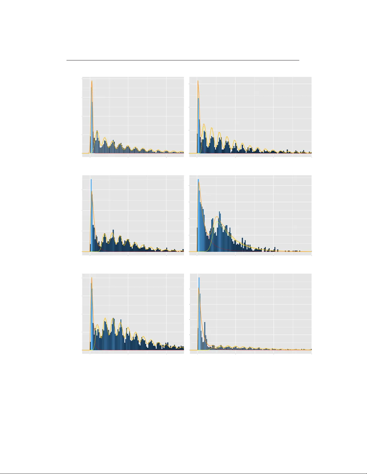
Mo delling Hospital length of sta y using convolutive mixtures distributions Adrien Ick o wicz, Ross Spa rks Abstract Length of hospital sta y (LOS) is an imp ortan t indicator of the hospital activit y and managemen t of health care. The sk ewness in the distribution of LOS p oses problems in statistical mo delling b ecause it fails to adequately follo w the usual traditional distribution suc h as the log-normal distribution. The aim of this work is to mo del the v ariable LOS using the con v olution of t w o distributions; a tec hnique w ell known in the signal pro cessing comm unit y . The sp ec ificit y of that mo del is that the v ariable of in terest is considered to b e the resulting sum of t w o random v ariables with different distributions. One of the v ariables will feature the patient- related factors in terms their need to recov er from their admission condition, while the other mo dels the hospital managemen t process suc h as the disc harging process. Tw o estimation procedures are prop osed. One is the classical maxim um lik eliho o d, while the other relates to the expectation maximisation algorithm. W e will present some results obtained by applying this mo del to a set of real data from a group of hospitals in Victoria (Australia). Keyw o rds: length of stay; negative binomial distribution; skewness; conv olution 1 Motivation of the study Length of stay (LOS) is an easily av ailable indicator of hospital activity . It is used for v arious purp oses, such as managemen t of hospital care, quality control, appro- priateness of hospital use and hospital planning. LOS is an indirect estimator of resources consumption and of the efficiency of one of the aspects of hospital patien t care: b ed managemen t. As such a quan tity of in terest, man y w orks hav e flourished with the aim of accurately estimate the LOS. Amongst these works, most start with the diagnosis-related group (DR G), that determines the amoun t of paymen t allo cated to the hospital. The DR Gs provide a classification system of episo des 1 1 Motivation of the study 2 of hospitalization with clinically recognized definitions, where it is exp ected that patien ts in the same class consume similar quantities of resources, as a result of a pro cess of similar hospital care. The mean of the LOS is used as an indicator of the consumption of resources b ecause of its a v ailabilit y and go o d relation with raised costs. Hence, we ma y sa y that DR Gs hav e b een partially created in order to get homogeneous groups with resp ect to the consumption of services and costs, closely related to LOS. The empirical distribution of LOS is well established to b e p ositively skew ed, m ulti-mo dal, to contain outliers and to significantly v ary b etw een DRGs [ 1 , 2 ]. This heterogeneit y of LOS p oses a problem for statistical analysis, limiting the use of inference techniques based on normalit y assumptions. Since a large num b er of DRGs m ust b e analyzed routinely , automatic pro cedures are needed for con- v enien tly treating sk ewness. Different transformations (e.g. the logarithmic one) of LOS hav e b een attempted to attain normality , and subsequently to apply the corresp onding tests [ 1 ], etc.). Ho w ev er, these approaches rely on the unrealistic homogeneit y assumption on the entire sample. Marazzi et al. [ 2 ] assessed the ad- equacy of three conv entional parametric mo dels, Lognormal (long-tailed), W eibull and Gamma (short-tailed), for describing the LOS distribution. But, as Lee et al. [ 3 ] p oin t out, none of them seemed to fit satisfactorily in a wide v ariet y of samples. The main issue is that the assumption of heterogeneous sub-p opulations would b e more appropriate than single DRG p opulations. Mixture distribution analysis can clarify whether or not a sk ewed distribution is comp osed of heterogeneous comp onents [ 4 ]. Re cen tly , Atienza [ 5 ] tried to mo del the LOS within DR Gs using a mixture of Gamma, W eibull and Lognormal distri- butions. The prop osed mo del sho ws goo d fitting prop erties but requires a complex EM algorithm that will b e extremely sensitive to initial v alues. Carter and P otts [ 6 ] use a purely negative binomial regression to fit their data on knee replacement. They displa y a relativ e efficiency of 75% for a v ery sp ecific LoS of 4 − 6 da ys, the margin error b eing 2 days. The results for other LoS were how ev er more disap- p oin ting. All these mo dels suffers from v arious limitations. The idea of fitting a mixture mo del has sev eral dra wbacks. It is computationally complex, esp ecially when the n um b er of mixtures is unkno wn. It lacks of natural in terpretation, in particular is the mo des of the mixture do not correspond to a simple combination of explana- tory v ariables. Moreo ver, all these works failed to describ e the exact b ehaviou r of the LOS. [Figure 1 ab out here.] Indeed, Figure 1 presents t wo histograms of the same LOS data, but with different breakp oin ts. On the left, the breakp oints are tak en every days, while they were 2 Mo delling principles 3 tak en ev ery 6 hours on the right histogram. [Figure 2 ab out here.] The ob jectiv e of our work is to analyse LOS using a new approach, where the fitting and the medical interpretation of the results are the t wo aims. Our mo del is defined as a mixture of tw o distributions, one describing the short stays, and one the long stays. Moreo v er, the idea driving the ”long-sta y” component is to consider the observ ation as the results of the sum of tw o random v ariables, one describing the recov ery p erio d, and the other describing the disc harge lag (link ed to the hos- pital pro cess). The ”short-stay” comp onen t, on the other hand, will b e fitted has a log-normal distribution as we assume that the disc harge lag will b e negligible. The results obtained in this w ork are of t w o kinds. First w e prov e that the fitting of the data obtained through this mo del is equiv alent to the b est existing fitting in the literature. Then, through regression results, we help identifying the features of influence on the disc harge lag, hence p ointing what is un usual in the hospital pro cess. The pap er is organized as follows. Section 2 con tains a theoretical exp o- sition of the mo delling principles: the mo del description, and the imp ortance of differen tiating b etw een the t w o effects. In Section 3 we presen t differen t estima- tion tec hniques. While the maximum likelihoo d remains the fa v ourite tec hnique, it can suffer from slowness. The Exp ectation-Maximisation algorithm, on the other hand, has go o d chances of reaching a lo cal maximum if the initialization is not prop erly defined. W e prop ose different options to sort this out. In Section 4.2 , w e apply this metho d to real LOS data from a hospital in Victoria (Australia). Finally , w e hav e included a short discussion on the prop osed metho dology . 2 Mo delling p rinciples The outcome v ariable LOS is usually defined to b e the num b er of (whole) days from admission to discharge. This assumption of an in teger v alue for the outcome v ariable limits the p ossible distributions that can b e used to fit a mo del to the data. Moreo v er, w e find this assumption to o restrictive to understand what part of the LOS is due to the disease, and what part is due to the hospital pro cess. By allo wing the LOS v ariable to b e contin uous (with time unit still b eing the day), w e sta y closer to the hospital reality . Let Y b e the random v ariable represen ting the length of sta y . W e hav e N obser- v ations, denoted ( y i ) i ≤ N . Eac h length of sta y is linked to a hospital admission record, pro viding additional information that can help in understanding the ran- dom b eha viour of Y . Let denote these complementary observ ations X . 2 Mo delling principles 4 2.1 The sho rt sta y / long sta y dichotomy The first mo delling idea in this pap er is to consider that the length of stay is follo wing a mixture distribution, that is, Y = π Y L + (1 − π ) Y S (1) where π is a random Bernoulli v ariable of unknown parameter v alue. Y L (resp ec- tiv ely Y S ) is the v ariable ass o ciated with the long stays (resp. short sta ys). This mo del is quite straightforw ard as we can observ e from Figure 1 that there is a bump in the distribution of the small stays, and quite a hea vy tail for long length of sta ys. Ho w ev er, this mo del is not accurate enough as it fails to capture the v ariations in the long sta ys. T o o v ercome this, we prop ose a second lay er in our mo del b y describing more accurately what we b elieve is the reco very pro cess. 2.2 The ”long-sta y” convolution mo del In our model, w e assume that Y L is the outcome of a t w o level pro cess. The first comp onen t, the patien t-disease related length of stay , will describe the reco very p e- rio d part of the LOS. The second comp onen t, related to the hospital management, will affect the daily v ariations of LOS. As such, we can write Y L , Y L = K + E (2) where K is a random v ariable on in teger v alues (for example, a negativ e binomial distribution), and E is a contin uous random v ariable (for example a Gaussian distribution). The regression principle is easily extensible to this case, and w e ha v e, E [ Y L | X ] = E [ K | X ] + E [ E | X ] (3) If w e denote f the densit y function, we then ha ve, f Y L | X ( y ) = Z f E | X ( y − k ) f K | X ( k ) d k (4) By assuming the conditional indep endence of the observ ations, the likelihoo d is simply defined as the pro duct of the densities defined in Eq. 4 incorp orated in to the mixture probabilit y . A detailed expression of the likelihoo d is given in section 3.1 . 2 Mo delling principles 5 As an example, using K as a Negativ e Binomial and E as a Gaussian, and replacing the densities with their expressions, we hav e, f Y L | X ( y ) = + ∞ X k =0 1 σ ( x ) p (2 π ) exp  − 1 2 σ ( x ) 2 ( y − k − m ( x )) 2  Γ( r ( x ) + k ) Γ( r ( x )) k ! p ( x ) r ( x ) (1 − p ( x )) k (5) As stated in the previous equation, the cov ariates X can b e of influence in any of the for parameters of the conv oluted distribution. T able 1 summarizes the mo delling assumptions w e are making by building a such mo del. [T able 1 ab out here.] This form ulation allo ws complex functions to b e fitted, also we will focus in this pap er on linear functions, s ( x ) = h ( β s X s ) (6) where s = { p, r , m, σ } and h will serv e as a transform to ensure the linear combi- nation do es not pro duce outb ound parameters. The combination of p ossible distributions is described below. F or the reco very p erio d, we can use: • The normal or the log-normal distribution, describ ed by their parameters µ and σ 2 , and which densities are f 1 ( x ) = 1 σ √ 2 π exp h − ( x − µ ) 2 2 σ 2 i and f 2 ( x ) = 1 x σ √ 2 π exp h − (ln x − µ ) 2 2 σ 2 i (7) F or the discharge lag, we can use: • The Negativ e Binomial distribution, described b y its parameters r and p , and whic h density is p 1 ( k ) = Γ( r + k ) Γ( r )Γ( k ) p r (1 − p ) k (8) This distribution is helpful to mo del ov er-disp ersion of counts data. • The Poisson distribution, describ ed by its parameter λ , and which densit y is p 2 ( k ) = λ k k ! exp[ − λ ] (9) The P oisson distribution is the most used distribution to mo del counts. 2 Mo delling principles 6 • The Conw ay Maxw ell Poisson distribution, described by its parameters λ and ν , and which density is p 3 ( k ) = λ k ( k !) ν 1 Z ( λ, ν ) (10) where Z () is a normalizing constan t. This distribution, well less forekno wn than the t w o previous ones, is useful to mo del under-disp ersion in coun ts data. Then, w e can also use distribution with b ounded supp ort, making the approach more lik e a classical mixture problem, • The Binomial distribution, describ ed b y its parameters n and p , and which densit y is p 4 ( k ) = C k n p k (1 − p ) n − k (11) • The Multinomial distribution, described b y its parameters p 1 to p K , where K + 1 is the maximum num b er of groups. Its densit y is p 5 ( k ) = p k (12) 2.3 Link with image p ro cessing This con volution-based approac h is nothing new in the signal pro cessing literature, in particular for the image pro cessing scientists. In their context, the conv olution mo del aims at describing the degradation of an image due to noise. One partic- ular model aims at describing the degradation in t w o components. The P oisson comp onen t, which relates to the quan tum nature of ligh ts, mo dels the impulsive noise, and the Gaussian comp onen t, whic h relates to the noise presen t in the elec- tronic part of the imaging system [see 7 – 9 ]. The aim of these approaches is to reco v er the image and estimate the noise parameters altogether. Different algo- rithms hav e b een dev elop ed to solve this inv erse problem, whic h is often describ ed b y the following equation, min x ∈ R N  f ( x ) = Φ( x ) + ρ ( x )  (13) where Φ stands for the data fidelity term, and ρ is a regularization function incor- p orating a priori information. In the Bay esian framework, this allows to compute the MAP estimate of the original signal x . In this context, the data fidelity term is defined as the negative logarithm of the lik eliho od and the regularization term corresp onds to the p otential of the chosen prior probabilit y densit y function. 3 Estimation procedure 7 In the context of this article, the original signal can be view ed as the disease- related length of stay b efore its degradation b y the hospital pro cess. Therefore, an estimation of the disease-related length of sta y would not only give an idea of the hospital stress (b y differentiating with the actual LoS) but could also b e used as a first-hand classification to ol for the disease. Not to mention the hospital managemen t ev olutions that can b e derived from such an information. 3 Estimation p ro cedure The study has a principal aim. W e w an t to forecast the LOS of a patient arriving in a hospital according to the information a v ailable up on arriv al. In order to refine the prediction, w e need to correctly identify the co v ariates of importance, and infer their influence. This will be done through the parameter estimation (maximum lik eliho o d estimation, in section 3.1 and exp ectation-maximisation algorithm, sec- tion 3.2 ), which will the allow for prediction. The mo del dev elop ed in this pap er mak es it also p ossible to iden tify the p ossible hospital stress. This is made possible b y the separation of the disease-patient related LOS from the delays due to the hospital pro cess. Therefore, b y carefully analysing the estimated parameters of the hospital-link ed features, we may b e able to identify the stress factors in the LOS, if existing. 3.1 Lik eliho o d based estimation With the notations from the previous section, and assuming that the LOS ob- serv ations are conditionally indep enden t from eac h other, we can write the log- lik eliho o d, log L ( y i =1 ...N | θ ) = X i log f θ ( y i ) = X i log h pf Y S | X ( y i ) + (1 − p ) f Y L | X ( y i ) i = X i log h pf Y S | X ( y i ) + (1 − p ) X k f E | X ( y − k ) f K | X ( k ) i (14) Maximizing Eq. 14 is a v ery hard task, that has to b e handled numerically [ 10 , 11 ]. But even numerically , the con vergence of the existing algorithms can be quite slo w, in particular when the dimension of X increases. W ager [ 12 ] proposes a geometrical approach for estimating the parameters, using the empirical distri- bution, whic h roughly matches the accuracy of fully general maxim um likelihoo d estimators at a fraction of the computational cost. 3 Estimation procedure 8 3.2 Exp ectation-maximisation (EM) algo rithm The baseline mo del we use b eing a mixture, a natural estimation pro cedure w ould b e the exp ectation-maximization (EM) algorithm. The EM algorithm[ 13 ] is the most p opular approach for calculating the maximum lik eliho o d estimator of latent v ariable mo dels. F or a thorough review on the estimation of mixture mo dels, see [ 14 – 16 ]. Ho w ev er, due to the nonconcavit y of the likelihoo d function of laten t v ariable models, the EM algorithm generally only con verges to a lo cal maxim um rather than the global one [ 17 ]. On the other hand, existing statistical guarantees for laten t v ariable mo dels are only established for global optima [ 18 ]. Let briefly review the classical EM algorithm. Giv en the observ ations ( y i ) i ≤ N , and an unobserved laten t v ariable Z ∈ Z , the algorithm aims at maximizing the augmen ted log-lik eliho o d ` N ( θ ) = X i log h θ ( y i ) where h θ ( y ) = Z Z f θ ( y , z ) d z (15) Because Z is unobserv ed, it is difficult to ev aluate ` N ( θ ). Instead, the EM maxi- mize Q N ( θ ; θ 0 ) = 1 N X i Z Z f θ ( z | y i ) log f θ ( y i , z ) d z (16) whic h is the difference betw een the optimal likelihoo d and a given lik eliho o d. In order to achiev e the maximisation, the EM pro ceeds in tw o steps during each iteration,      (E) Compute f θ ( z | y i ) (M) Set θ ( c +1) = argmax θ Q N ( θ , θ ( c ) ) (17) In the context of this article, Z will describ e the short or long sta ys, meaning Z = { 0 , 1 } . With the previous notations, we would also ha ve, f θ ( z = 0 | y i ) ∝ p ( z = 0) × f Y S | X ( y i ) and f θ ( z = 1 | y i ) ∝ p ( z = 1) × X k f E | X ( y − k ) f K | X ( k ) (18) whic h will b e normalised to keep the right prop erties, and f θ ( y i , z ) = Z Z f θ ( y i | z ) p ( z ) d z (19) 3.3 Tw o-dimensional Exp ectation-maximisation (2d-EM) algo rithm A differen t in terpretation of the mo del can also lead to the idea of a double EM algorithm. Indeed, the mo del stated in eq. 1 decrib es the mixture of tw o distribu- tions, one of them b eing also a mixture (while infinite, it is a mixture, sometimes 3 Estimation procedure 9 also called conv olution). In this double mixture mo del framework, we increase the dimension of the laten t v ariable, so that Z = ( C , S ) ∈ C × S . If C and S were indep enden t, the problem would w e the same as a normal latent v ariable problem. Ho w ev er, tw o differences exist here. First, C and S are not indep endent. Also, C = N , making one of the mixture infinite. The main driver b ehind that in terpre- tation of the mo del is the conv olution distribution in the following equation, X k f E | X ( y − k ) f K | X ( k ) (20) This probability density function can b e long to calculate, in particular when k ∈ N . T o a v oid this additional computational complexity , w e will use this double EM to use only analytical density functions. The literature on infinite mixtures finds solution in the Ba y esian comm unit y w ork- ing on Gaussian processes [ 19 , 20 ]. While a maximum lik eliho o d estimation is quite common in finite mixture problems [ 21 ], its generalization to infinite mixture is not straightforw ard. Using Gaussian and Dirichlet pro cesses, Sun [ 22 ] prop oses differen t inference techniques to fit the mo del. In the end, all the prop osed meth- o ds refers to the EM algorithm as a wa y to deal with the incomplete nature of the data. Moulines [ 23 ] briefly mentions the link b et ween deconv olution and mixture, prop osing an EM algorithm to estimate b oth the noise and the signal parameters. The link with the mixtures is quite ten uous because of the infinite nature of the sum in the likelihoo d equation. Moreo v er, the usual mixture definition implies an empirical estimation of the mixture probabilities, which mak e the infinite as- sumption imp ossible to estimate. How ever, with a parametric assumption on the mixture w eigh ts, it b ecomes theoretically and practically possible. F ollo wing the change in the latent v ariable dimension, we can rewrite Q , Q N ( θ ; θ 0 ) = 1 N X i Z C Z S f θ ( c , s | y i ) log f θ ( y i , c , s ) d c d s (21) In this expression, w e still need to calculate the t w o terms. First, w e recall that w e can re-write f θ ( y i , c , s ) = f θ ( y i | c , s ) × f θ ( c | s ) × f θ ( s ) (22) f θ ( s ) is the mixing parameter (defining the absolute probabilit y of s ) that will b e non-parametrically estimated using the standard EM pro cedure for the mixing co efficien ts. Then we calculate f θ ( c | s ) suc h that, ∀ c ∈ C ,  f θ ( c | s = 0) = δ 1 ( c ) f θ ( c | s = 1) = f K | X ( c ) (23) 4 Results 10 Iden tically , w e define f θ ( y i | c , s ), ∀ c ∈ C ,  f θ ( y i | c , s = 0) = f Y S | X ( y i ) f θ ( y i | c , s = 1) = f E | X ( y i − c ) (24) Finally , w e ha v e to calculate f θ ( c , s | y i ). Because s and c are not indep enden t, w e use once again the conditioning (and the Ba yes paradigm), yielding, f θ ( c , s | y i ) ∝ f θ ( y i | c , s ) × f θ ( c | s ) × f θ ( s ) (25) Thanks to Eqs. 23 and 24 , w e can achiev e our algorithm. W e can no w define the follo wing three steps of the algorithm,        (E-1) Compute f θ ( s | y i ) (E-2) Compute f θ ( c | y i , c ) (M) Set θ ( c +1) = argmax θ Q N ( θ , θ ( c ) ) (26) 4 Results 4.1 Fitting: Comparison with p revious studies In [ 5 ] the authors fit a (finite) mixture of differen t distributions (Gamma, W eibull, Lognormal) to the data from different DRGs. In order to compare our mo del to theirs, w e will use our data issued from the same DRGs: • DRG 14: Sp ecific cerebrov ascular disorders except transien t ischemic attac k (DR Gs B 70 in our data); • DRG 88: Chronic obstructive pulmonary disease (DR G E 65 B in our data); • DRG 122: Circulatory disorders with acute my o cardial infarction without cardio v ascular complications, disc harged alive (DRG F 60 B in our data); • DRG 127: Heart failure and shock (DRGs F 62 A and F 62 B in our data); • DRG 541: Respiratory diseases except infection, bronc hitis and asthma (DR Gs E 02, E 40, E 41 Z , E 64, E 67, E 71, E 75, E 76 Z in our data), and compute a discrepancy measure. As a discrepancy measure betw een the em- pirical F θ e ( . ) and the estimated distribution function F ˆ θ ( . ), the uniform measure [ 24 ], also called Kolmogorov measure, is prop osed: d ( θ e , ˆ θ ) = sup x ∈ R | F θ e ( x ) − F ˆ θ ( x ) | (27) The results are presen ted in T able 2 , for different distributions and the prop osed DR Gs. 4 Results 11 [T able 2 ab out here.] Amongst the fitted distributions, w e choose the most p opular choices, namely the Log-normal, the Gamma and the W eibull distribution. Moreov er, w e compare our p erformance with the b est existing in the literature, the mo del prop osed in [ 5 ]. The prop osed model is the chosen to b e the b est fit amongst the com bination of P oisson-Negativ e Binomial-CoMPoisson and Gaussian-Log Normal. It can also b e c hosen amongst the combination of Binomial and Multinomial distributions. The main diffe rence b etw een these models is the nature of the discrete distribution (and hence the mixture), which has an infinite supp ort in the first case and a finite supp ort in the later. The choice of the mo del has a significan t influence and has to be made with a purpose in mind. F or a better fitting and understand, the Multinomial approac h can pro ve very useful. How ever, if the aim is the forecast, the infinite mixture may prov e more robust, in particular in situations where few data are av ailable. As we can see from the table, the results of our model are outp erforming the results of the model prop osed in [ 5 ], except the distribution in DR G 127 where the results can b e considered equiv alent. W e also displa y in Figure 3 the densit y histograms for the 5 DRGs (subplots (a) for all DR Gs, (b)-(f ) for eac h individual DRG), with curves representing the estimated distributions. [Figure 3 ab out here.] 4.2 Understanding: Explaining LOS variations List of features The interpretation of our statistical mo delling is to consider that a particular dis- ease on a particular patien t will need to b e treated in a num b er of day that will b e distributed as the recov ery p erio d. Then, additional noise is considered, due to the hospital processes, that will b e distributed according to a distribution whose supp ort will b e finite or infinite. T o fit that mo del, we hav e the features presented in T able 3 . [T able 3 ab out here.] W e also ha v e made a n um b er of assumption that will limit the num b er of parameters to b e estimated. This is safer, as the estimation pro cedure can tak e a long time and some features hav e some really prohibitiv e dimensions. This list is: - The probability that a sta y is a short or long sta y cannot b e explained by the av ailable feature. This assumption is probably the w eakest assumption 4 Results 12 (in terms of mo delling) as it seems ob vious that DR G, or Admission Unit will b e imp ortant. This is clearly an assumption that will b e remo v ed in further w ork. - The short stay parameters (mean and v ariance) will not dep end on an y of the av ailable features. This modelling assumption is based on the fact that the v ery small v ariance of that distribution makes it useless to fit features. - F or the same reasons, the v ariance of the recov ery p erio d of the long stays comp onen t will not dep end on any of the av ailable features either. F or many reasons, the DR G cannot b e used as is into the mo del. T o ov ercome that problem, the data can b e analysed by DR G, as w e did in the previous section, or, more safely , b y considering an in termediate kind of information. F or example, the use of the first tw o letters of the DRG co de can prov e useful and not to o v ast. Results and discussion The results of the mo del for the 5 DRGs altogether are presented in T able 5 . W e observ e in particular the sp ecifics for the 5 selected DRGs in T able 4 [T able 4 ab out here.] 4 Results 13 [T able 5 ab out here.] 5 Discussion 14 5 Discussion W e presented in this article a new mo del of hospital length of stay data. This new mo del pro vides a b etter fitting of the data, and also giv es a realistic description of the pro cess pro ducing the length of stay . W e strongly b elieve that this mo del will pro v e useful for clinicians and hospital managers in their attempt to improv e the patien ts and the medical staff exp erience. This mo del is complex to estimate, due to the mixture and the conv olution. The maxim um lik eliho o d approac h is prop osed, and is able to estimate the parameters correctly . How ever, it cannot tell us if the patient’s stay belong to the short or the long category . This kind of information w ould typically b e useful to iden tify outliers, or to p erform additional statistical analysis on one or the other category . F or this reason, w e used the classical EM algorithm [ 13 ]. W e faced another c hal- lenge with this estimation pro cedure, b ecause the con v olution distribution optimal solution can only b e calculated numerically , which leads to extended delays in the optimisation pro cedure. T o o v ercome this, we considered the con v olution as an infinite mixture, where the mixture co efficient are parametrically defined. T o p er- form the estimation, we proposed an augmen ted EM algorithm called 2d-EM. In this algorithm, w e consider that the dimension of the latent space is equal to 2. This allows more flexibility in the mo del, while the computational complexity re- mains manageable. Finally , w e applied it to real data from Melbourne (Australia). W e iden tify imp ortant v ariables for the purp ose of length of stay mo delling. Another aspect that m ust be discussed is that the prop osed mo del is a complicated one. As researc h scien tists w orking with real w orld problems, we hav e to mak e a decision betw een the complexit y of the model / computation procedure and the fit- ting of the data / me aningfulness of the mo del. F or this mo del, the computational effort and the complexity should not b e considered as excessiv e. F urthermore, this metho dology seems more adequate for the DRGs w e hav e w orked on. The model based on a unique family of distributions is less complex but has tw o dra wbac ks. First, the necessit y of previously selecting the family among the most usual asym- metric distributions. Second, the results pro vided are less optimal. Therefore, the study of a simpler mo del do es not imply either a significan t reduction of the computational effort or b etter results. A few more words on the understanding of the prop osed mo del are needed. First, regarding the optimalit y of the solution obtained b y maximising the likelihoo d. A t b est, w e hav e four parameters that need to b e fitted. In some particular situation, that ma y lead to an ov erfitting of the data. W e recommend the user to pa y atten- tion to the results, and any prior kno wledge about the data should b e considered with care. F or example, the v ariance of the second distribution of the long stay mo del (usually a Gaussian distribution) can b e sp ecified, so that the estimation 5 Discussion 15 pro cedure ends quic ker with an appropriate fit. Or at least, specify bounds in whic h that parameter should b elong. The same careful consideration m ust lead the choice of the features and whic h v ariable ( K or E ) they should b e fitted in. Not only the estimation results will b e impacted, but also their in terpretations. In conclusion, we b eliev e that this work contributes to the developmen t of the statistical analysis of LOS distributions and other consumption v ariables in health services. Also this approach can be applied to other asymmetric data (for instance, the length of wait for surgical pro cedures or for medical attention). Ackno wledgement The authors would lik e to ackno wledge the financial supp ort of Common w ealth Health Department for the pro ject and in-kind op erational supp ort from Austin Health and the Roy al Melb ourne Hospital. References 1. Shach tman RH, Snapinn SM, Quade D, F reund Da, Kronhaus aK. A method for constructing case-mix indexes, with application to hospital length of sta y . He alth servic es r ese ar ch F eb 1986; 20 (6 Pt 1):737–62. URL http://www.pubmedcentral.nih.gov/articlerender. fcgi?artid=1068925&tool=pmcentrez&rendertype=abstract . 2. Marazzi a, Paccaud F, Ruffieux C, Beguin C. Fitting the distributions of length of stay by parametric mo dels. Me dic al c ar e Jun 1998; 36 (6):915–27. URL http://www.ncbi.nlm.nih.gov/pubmed/9630132 . 3. Lee A, Ng A, Y au K. Determinan ts of maternit y length of sta y: a gamma mixture risk-adjusted mo del. He alth c ar e management scienc e Dec 2001; 4 (4):249–55. URL http://www.ncbi.nlm.nih.gov/pubmed/11718457http: //link.springer.com/article/10.1023/A:1011810326113 . 4. Quantin C, Sauleau E, Bolard P . Mo deling of high-cost patien t distri- bution within renal failure diagnosis related group. Journal of clinic al Epidemiolo gy Mar 1999; 52 (3):251–8. URL http://www.ncbi.nlm.nih.gov/ pubmed/10210243http://www.sciencedirect.com/science/article/pii/ S0895435698001644 . 5. Atienza N. An application of mixture distributions in mo delization of length of hospital sta y. Statistics in me dicine Apr 2008; 27 (9):1403–20, doi:10.1002/ 5 Discussion 16 sim.3029. URL http://www.ncbi.nlm.nih.gov/pubmed/17680551http:// onlinelibrary.wiley.com/doi/10.1002/sim.3029/abstract . 6. Carter EM, Potts HWW. Predicting length of stay from an electronic patien t record system: a primary total knee replacement example. BMC me dic al infor- matics and de cision making Jan 2014; 14 (1):26, doi:10.1186/1472- 6947- 14- 26. URL http://www.pubmedcentral.nih.gov/articlerender.fcgi?artid= 3992140&tool=pmcentrez&rendertype=abstract . 7. Jeziersk a A, Chouzenoux E, P esquet J, T alb ot H. A conv ex approac h for image restoration with exact P oisson-Gaussian likelihoo d 2013; :1–12URL http:// hal.archives- ouvertes.fr/hal- 00922151/ . 8. Xiao Y, Zeng T, Y u J, Ng M. Restoration of images corrupted by mixed Gaussian-impulse noise via l 1 l 0 minimization. Pattern R e c o gnition Aug 2011; 44 (8):1708–1720, doi:10.1016/j.patcog.2011.02.002. URL http: //linkinghub.elsevier.com/retrieve/pii/S0031320311000495http: //www.sciencedirect.com/science/article/pii/S0031320311000495 . 9. Y an M. Restoration of images corrupted b y impulse noise and mixed Gaus- sian impulse noise using blind inpainting. SIAM Journal on Imaging Sci- enc es Apr 2013; :18doi:10.1137/12087178X. URL 1304.1408http://epubs.siam.org/doi/abs/10.1137/12087178X . 10. Simar L. Maximum likelihoo d estimation of a comp ound Poisson pro cess. The Annals of Statistics 1976; 4 (6):1200–1209. URL http://www.jstor.org/ stable/2958588 . 11. Sprott D. Estimating the parameters of a conv olution b y maximum lik eli- ho o d. Journal of the Americ an Statistic al Asso ciation 1983; 78 (382):457– 460. URL http://amstat.tandfonline.com/doi/abs/10.1080/01621459. 1983.10477994 . 12. W ager S. A geometric approach to density estimation with additiv e noise. Statistic a Sinic a 2013; :1–21URL http://www3.stat.sinica.edu.tw/ss_ newpaper/SS- 12- 355_na.pdf . 13. Dempster AP , Laird NM, Rubin DB, Url S, So ciety RS, So ciety RS. Maxi- m um lik eliho o d from incomplete data via the EM algorithm. Journal of the R oyal Statistic al So ciety. Series B (Metho dolo gic al) 1977; 39 (1):1–38, doi: 10.1.1.133.4884. URL http://citeseerx.ist.psu.edu/viewdoc/summary? doi=10.1.1.133.4884 . 5 Discussion 17 14. Redner R, W alker H. Mixture densities, maximum likelihoo d and the EM algorithm. SIAM r eview 1984; 26 (2):195–239. URL http://epubs.siam.org/ doi/abs/10.1137/1026034 . 15. Bilmes J. A gentle tutorial of the EM algorithm and its application to pa- rameter estimation for Gaussian mixture and hidden Mark o v mo dels. In- ternational Computer Scienc e Institute 1998; URL http://lasa.epfl.ch/ teaching/lectures/ML_Phd/Notes/GP- GMM.pdf . 16. Marin J, Mengersen K, Rob ert C. Bay esian mo delling and inference on mixtures of distributions. Handb o ok of statistics 2005; URL http://www. sciencedirect.com/science/article/pii/S0169716105250162 . 17. W u CFJ. On the Con vergence Prop erties of the EM Algorithm 1983. 18. Bartholomew DJ, Knott M, Moustaki I. Laten t v ariable models and factor analysis: a unified approach. T e chnometrics 2011; 43 :111–111. 19. Rasmussen C. The infinite Gaussian mixture mo del. NIPS , 1999; 554– 560. URL http://www.kyb.tue.mpg.de/fileadmin/user_upload/files/ publications/pdfs/pdf2299.pdf . 20. Rasmussen C, Ghahramani Z. Infinite mixtures of Gaussian pro- cess exp erts. A dvanc es in neur al information . . . 2002; URL http: //books.google.com/books?hl=en&lr=&id=GbC8cqxGR7YC&oi=fnd&pg= PA881&dq=Infinite+Mixtures+of+Gaussian+Process+Experts&ots= ZwJ- K6- EA6&sig=fKiRC1VrQK6- j_ti_aXCuEe0hN4 . 21. Zhang C. Generalized maximum lik eliho o d estimation of nor- mal mixture densities. Statistic a Sinic a 2009; 19 :1297–1318. URL http://epubs.siam.org/doi/pdf/10.1137/1111003http://www3.stat. sinica.edu.tw/statistica/password.asp?vol=19&num=3&art=23 . 22. Sun S, Xu X. V ariational inference for infinite mixtures of Gaussian pro cesses with applications to traffic flo w prediction. Intel ligent T r ansp ortation Systems, IEEE . . . Jun 2011; 12 (2):466–475, doi:10.1109/TITS.2010.2093575. URL http://ieeexplore.ieee.org/lpdocs/epic03/wrapper.htm?arnumber= 5664792http://ieeexplore.ieee.org/xpls/abs_all.jsp?arnumber= 5664792 . 23. Moulines E, Cardoso J, Gassiat E. Maximum likelihoo d for blind sepa- ration and deconv olution of noisy signals using mixture models. Interna- tional Conferne c e on A c c oustic, Sp e e ch, and Signal Pr o c essing , 1997. URL http://ieeexplore.ieee.org/xpls/abs_all.jsp?arnumber=604649 . 5 Discussion 18 24. Zolotarev V. Probability metrics. T e oriya V er oyatnostei i e e Primeneniya 1983; 28 (2):264–287. URL http://www.mathnet.ru/eng/tvp2295 . T ABLES 19 T ab. 1: Example of mo del description, with a Negative Binomial and a Nor- mal distribution. P arameter Parameter Interpreta- tion Ex. of v ariable V ariable In terpretation p ( x ) Probabilit y of success Admission da y On a w eekday , more n urses and do ctors can sign up on the dis- c harge. r ( x ) Number of failures b e- fore success Care t yp e Dep ending on the care type, m ul- tiple exams may hav e to b e made, hence an increased lag. m ( x ) Av erage reco very perio d DR G A patien t with a particular dis- ease type is exp ected to recov er in m days. σ ( x ) V ariation of reco v ery p erio d P atien t age Older patien ts may ha ve more v ariation in their recov ery p e- rio d. T ABLES 20 T ab. 2: Measure of distance b etw een the estimated distribution and the empirical distribution. Mo del All 5 DRGs DRG 14 DRG 88 DRG 122 DR G 127 DRG 541 Lognormal 0.096 0.045 0.112 0.111 0.086 0.087 Gamma 0.064 0.107 0.076 0.123 0.114 0.139 W eibull 0.063 0.077 0.063 0.092 0.077 0.091 Mixture [ 5 ] 0.023 0.018 0.049 0.108 0.017 0.054 Prop osed mo del 0.019 0.011 0.016 0.023 0.019 0.022 T ABLES 21 T ab. 3: T able of p ossible explanatory v ariable for LoS. (a) P atien t related features F eature name feature t yp e dimension Age n umerical . Gender categorical 3 Marital Status categorical 4 Ethnicit y categorical 5 Coun try categorical 50 Disease T yp e categorical 9 DR G categorical 634 (b) Hospital related features F eature name feature t yp e dimension Hour of arriv al n umerical . Da y of arriv al categorical 7 Mon th of arriv al numerical . Admission T yp e categorical 4 Admission Unit categorical 46 Disc harge Unit categorical 46 Care T yp e categorical 4 T ABLES 22 T ab. 4: Numerical results of the mo del, with the repartition b etw een short and long stay ers, and the prop erties of these stays. Short sta y ers Long sta y ers % mean sd % mean sd DR G 14 20.4 6 hours 3 hours 79.6 4 days, 10 hours 3 da ys, 10 hours DR G 88 24.8 7 hours 3 hours 75.2 4 days, 11 hours 2 da ys, 20 hours DR G 122 45.6 17 hours 11 hours 54.4 4 days, 4 hours 2 da ys DR G 127 14.9 7 hours 3.5 hours 85.1 4 days, 23 hours 3 da ys, 6 hours DR G 541 63.0 13 hours 11 hours 37.0 6 da ys, 14 hours 3 da ys, 14 hours T ABLES 23 T ab. 5: Results of the regression mo del for the 5 selected DR Gs. The four results presented provide the influence of the predictors on (a) the probabilit y of ha ving a short sta y , (b) the short sta y duration, (c) the reco v ery p erio d duration (long sta y comp onent) (d) the disc harge lag (long sta y comp onen t). (a) Logistic regression results Name Mean 95% CI bs(Age)2 − 8 − 6 − 4 − 2 0 2 4 6 − 2 . 46 ( − 3 . 01 to − 1 . 91) bs(Age)3 − 0 . 58 ( − 1 . 14 to − 0 . 02) DoWThursday 0 . 19 ( +0 . 02 to +0 . 36) DoWT uesday 0 . 17 ( +0 . 01 to +0 . 33) DiseaseTypesCorr2 − 0 . 98 ( − 1 . 08 to − 0 . 87) DiseaseTypesCorr3 − 2 . 13 ( − 2 . 28 to − 1 . 97) DiseaseTypesCorr4 − 2 . 94 ( − 3 . 19 to − 2 . 69) DiseaseTypesCorr5 − 3 . 66 ( − 4 . 10 to − 3 . 22) DiseaseTypesCorr6 − 3 . 53 ( − 4 . 14 to − 2 . 92) DiseaseTypesCorr7 − 5 . 23 ( − 7 . 24 to − 3 . 23) CountryNameEritrea 3 . 18 ( +0 . 05 to +6 . 32) CountryNameNorthernIreland 3 . 28 ( +0 . 48 to +6 . 07) (b) Log-normal regression results Name Mean 95% CI bs(Age)2 − 1 0 1 2 3 1 . 04 ( +0 . 54 to +1 . 54) bs(Age)3 0 . 79 ( +0 . 24 to +1 . 34) MoA03 − 0 . 44 ( − 0 . 67 to − 0 . 21) MoA10 − 0 . 23 ( − 0 . 42 to − 0 . 05) MoA12 − 0 . 29 ( − 0 . 49 to − 0 . 08) DoWSaturday − 0 . 20 ( − 0 . 36 to − 0 . 05) DoWSunday − 0 . 19 ( − 0 . 35 to − 0 . 03) DiseaseTypesCorr2 0 . 67 ( +0 . 55 to +0 . 80) DiseaseTypesCorr3 1 . 60 ( +1 . 08 to +2 . 13) AdmissionUnitCorr.initCardioThoracicSurgery 1 . 40 ( +0 . 42 to +2 . 38) AdmissionUnitCorr.initEmergency 1 . 22 ( +0 . 63 to +1 . 81) AdmissionUnitCorr.initInfectiousDiseases 2 . 69 ( +1 . 99 to +3 . 38) AdmissionUnitCorr.initNeurology 1 . 28 ( +0 . 34 to +2 . 22) AdmissionUnitCorr.initRespiratoryMedicine 1 . 01 ( +0 . 36 to +1 . 67) AdmissionUnitCorr.initStrokeUnit 0 . 97 ( +0 . 06 to +1 . 87) (c) Reco v ery p erio d regression Name Mean 95% CI DiseaseTypesCorr3 − 1 0 1 2 3 4 5 0 . 65 ( +0 . 48 to +0 . 83) DiseaseTypesCorr4 0 . 81 ( +0 . 63 to +0 . 99) DiseaseTypesCorr5 1 . 56 ( +1 . 36 to +1 . 76) DiseaseTypesCorr6 1 . 49 ( +1 . 23 to +1 . 75) DiseaseTypesCorr7 2 . 54 ( +2 . 29 to +2 . 79) DiseaseTypesCorr8 4 . 02 ( +3 . 51 to +4 . 53) DiseaseTypesCorr9 4 . 75 ( +4 . 23 to +5 . 26) CountryNameCorrAustria − 0 . 41 ( − 0 . 81 to − 0 . 02) CountryNameCorrLithuania 0 . 92 ( +0 . 51 to +1 . 34) CountryNameCorrUkraine − 0 . 37 ( − 0 . 67 to − 0 . 07) MaritalStatusNameCorrSingle − 0 . 19 ( − 0 . 32 to − 0 . 07) Intercept.sigma2 − 0 . 90 ( − 0 . 96 to − 0 . 84) (d) Disc harge lag regression Name Mean 95% CI Intercept.mu1 − 2 0 2 2 . 26 ( +1 . 27 to +3 . 26) DoWSunday − 0 . 12 ( − 0 . 22 to − 0 . 03) AdmissionUnitCorr.initCardiology − 0 . 83 ( − 1 . 37 to − 0 . 29) AdmissionUnitCorr.initCardioThoracicSurgery − 0 . 72 ( − 1 . 20 to − 0 . 24) AdmissionUnitCorr.initDialysis − 0 . 86 ( − 1 . 64 to − 0 . 08) AdmissionUnitCorr.initEmergency − 0 . 51 ( − 0 . 90 to − 0 . 12) AdmissionUnitCorr.initOtolaryngologyHeadNeck − 1 . 88 ( − 3 . 33 to − 0 . 43) Intercept.sigma1 0 . 14 ( +0 . 09 to +0 . 19) T ABLES 24 0.00 0.25 0.50 0.75 0.0 2.5 5.0 7.5 10.0 Length of stay density 0.0 0.5 1.0 1.5 2.0 2.5 0.0 2.5 5.0 7.5 10.0 Length of stay density Fig. 1: Comparison b et w een t w o histograms of the same data. On the left, break p oints are every da y . On the righ t, break p oin ts are every 6 hours. T ABLES 25 0 10000 20000 30000 40000 50000 00 01 02 03 04 05 06 07 08 09 10 11 12 13 14 15 16 17 18 19 20 21 22 23 Hour of arrival count 0 10000 20000 30000 40000 50000 00 01 02 03 04 05 06 07 08 09 10 11 12 13 14 15 16 17 18 19 20 21 22 23 Hour of departure count 00 01 02 03 04 05 06 07 08 09 10 11 12 13 14 15 16 17 18 19 20 21 22 23 00 01 02 03 04 05 06 07 08 09 10 11 12 13 14 15 16 17 18 19 20 21 22 23 HoA HoD 2.5 5.0 7.5 log(Freq) Fig. 2: Comparison b etw een time of arriv al, time of disc harge, and relation- ship betw een the t wo. T ABLES 26 0.0 0.2 0.4 0.6 0.8 0 5 10 15 Length of stay density (a) F ull data fitting 0.0 0.2 0.4 0.6 0 5 10 15 Length of stay density (b) DR G 14 0.0 0.2 0.4 0.6 0 5 10 15 Length of stay density (c) DR G 88 0.0 0.1 0.2 0.3 0.4 0 5 10 15 Length of stay density (d) DR G 122 0.0 0.1 0.2 0.3 0.4 0 5 10 15 Length of stay density (e) DR G 127 0.00 0.25 0.50 0.75 1.00 0 5 10 15 Length of stay density (f ) DRG 541 Fig. 3: Graphics on the mo delization of LOS v ariable for sev eral DR Gs. (b)- (f ): fitting of the estimated distribution and histogram of observ ations for eac h individual DR G. (a) Fitting for all the data. The y ello w lines represen t the long sta y distributions, and the red lines the short stay distributions.