CrossCat: A Fully Bayesian Nonparametric Method for Analyzing Heterogeneous, High Dimensional Data

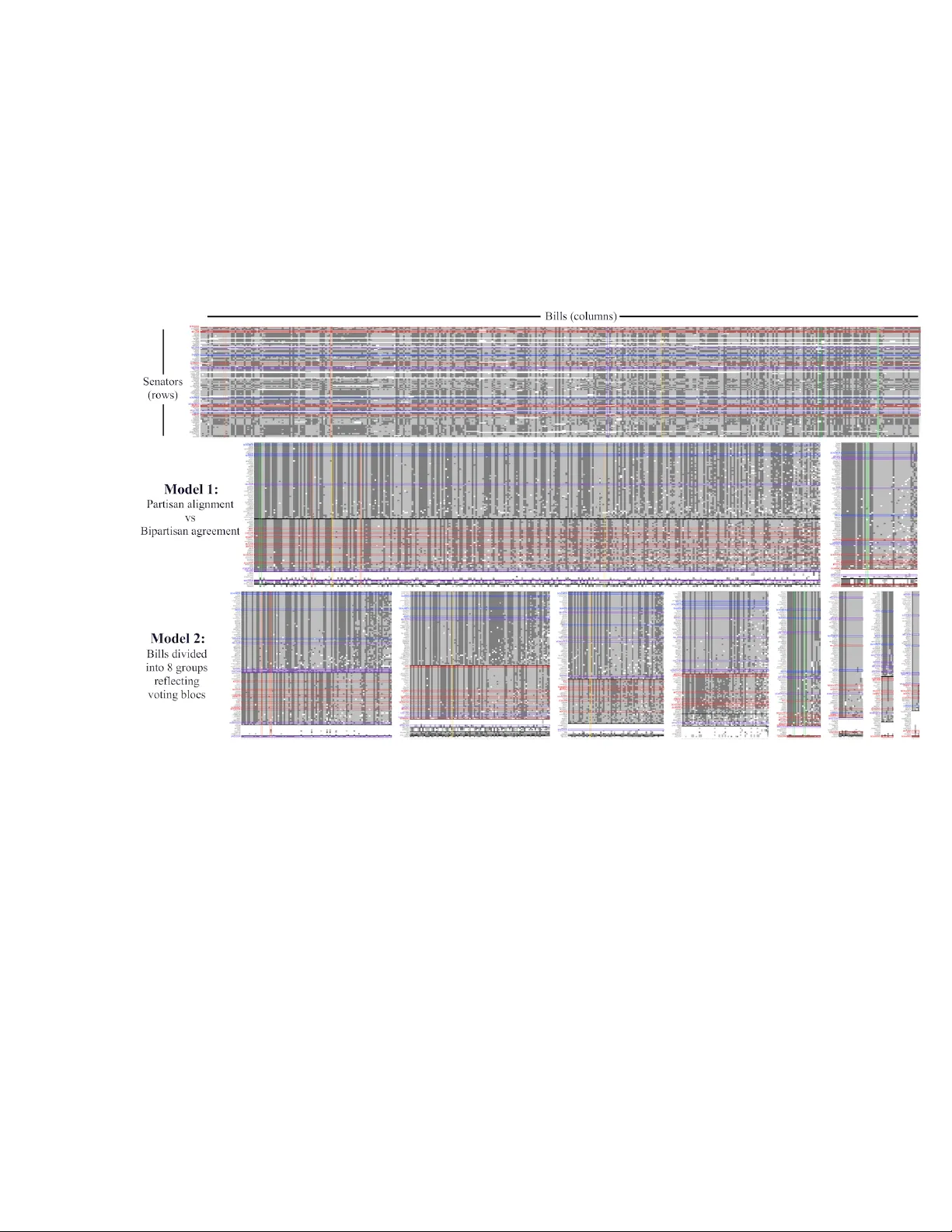
Cr ossCat: A Fully Bayesian Nonparametric Method f or Analyzing Heter ogeneous, High Dimensional Data V ikash Mansinghka V K M @ M I T . E D U Patrick Shafto P . S H A FT O @ L O U I S V I L L E . E D U Eric Jonas J O NA S @ P R I O R K N O W L E D G E . N E T Cap Petschulat C A P @ P R I O R K N OW L E D G E . N E T Max Gasner M A X @ P R I O R K N OW L E D G E . N E T Joshua B. T enenbaum J B T @ M I T . E D U Editor: David Blei Abstract There is a widespread need for statistical methods that can analyze high-dimensional datasets with- out imposing restrictiv e or opaque modeling assumptions. This paper describes a domain-general data analysis method called CrossCat. CrossCat infers multiple non-overlapping vie ws of the data, each consisting of a subset of the variables, and uses a separate nonparametric mixture to model each view . CrossCat is based on approximately Bayesian inference in a hierarchical, nonparamet- ric model for data tables. This model consists of a Dirichlet process mixture over the columns of a data table in which each mixture component is itself an independent Dirichlet process mixture ov er the ro ws; the inner mixture components are simple parametric models whose form depends on the types of data in the table. CrossCat combines strengths of mixture modeling and Bayesian net- work structure learning. Like mixture modeling, CrossCat can model a broad class of distrib utions by positing latent variables, and produces representations that can be efﬁciently conditioned and sampled from for prediction. Like Bayesian networks, CrossCat represents the dependencies and independencies between variables, and thus remains accurate when there are multiple statistical signals. Inference is done via a scalable Gibbs sampling scheme; this paper shows that it works well in practice. This paper also includes empirical results on heterogeneous tabular data of up to 10 million cells, such as hospital cost and quality measures, voting records, unemployment rates, gene expression measurements, and images of handwritten digits. CrossCat infers structure that is consistent with accepted ﬁndings and common-sense kno wledge in multiple domains and yields predictiv e accurac y competiti ve with generati ve, discriminativ e, and model-free alternati ves. Keyw ords: Bayesian nonparametrics, Dirichlet processes, Markov chain Monte Carlo, multiv ari- ate analysis, structure learning, unsupervised learning, semi-supervised learning Acknowledgments: The authors thank Ke vin Murphy , Ryan Rifkin, Cameron Freer, Daniel Roy , Bill Lazarus, Da vid Jensen, Beau Cronin, Rax Dillon, and the anonymous re vie wers and editor for v aluable suggestions. This work was supported in part by gifts from Google, NTT Commu- nication Sciences Laboratory , and Eli Lilly & Co; by the Army Research Ofﬁce under agreement number W911NF-13-1-0212; and by D ARP A via the XD A T A and PP AML programs. Any opin- ions, ﬁndings, and conclusions or recommendations expressed in this work are those of the authors and do not necessarily reﬂect the vie ws of any of the abo ve sponsors. 1 1. Introduction High-dimensional datasets containing data of multiple types hav e become commonplace. These datasets are often represented as tables, where ro ws correspond to data v ectors, columns correspond to observable v ariables or features, and the whole table is treated as a random subsample from a statistical population (Hastie, Tibshirani, Friedman, and Franklin, 2005). This setting brings new opportunities as well as new statistical challenges (NRC Committee on the Analysis of Massiv e Data, 2013; W asserman, 2011). In principle, the dimensionality and co verage of some of these datasets is sufﬁcient to rigorously answer to ﬁne-grained questions about small sub-populations. This size and richness also enables the detection of subtle predictiv e relationships, including those that depend on aggregating individually weak signals from large numbers of v ariables. Challenges include inte grating data of heterogeneous types (NRC Committee on the Analysis of Massiv e Data, 2013), suppressing spurious patterns (Benjamini and Hochberg, 1995; Attia, Ioannidis, et al., 2009), selecting features (W asserman, 2011; W eston, Mukherjee, et al., 2001), and the prev alence of non- ignorable missing data. This paper describes CrossCat, a general-purpose Bayesian method for analyzing high-dimensional mixed-type datasets that aims to mitigate these challenges. CrossCat is based on approximate in- ference in a hierarchical, nonparametric Bayesian model. This model is comprised of an “outer” Dirichlet process mixture over the columns of a table, with components that are themselves inde- pendent “inner” Dirichlet process mixture models over the rows. CrossCat is parameterized on a per-table basis by data type speciﬁc component models — for example, Beta-Bernoulli models for binary values and Normal-Gamma models for numerical values. Each “inner” mixture is solely re- sponsible for modeling a subset of the variables. Each hypothesis assumes a speciﬁc set of marginal dependencies and independencies. This formulation supports scalable algorithms for learning and prediction, speciﬁcally a collapsed MCMC scheme that marginalizes out all but the latent discrete state and hyper parameters. The name “CrossCat” is derived from the combinatorial skeleton of this probabilistic model. Each approximate posterior sample represents a cr oss-cate gorization of the input data table. In a cross-categorization, the variables are partitioned into a set of vie ws , with a separate partition of the entities into cate gories with respect to the v ariables in each view . Each ( ca t e gor y , var iabl e ) pair contains the sufﬁcient statistics or latent state needed by its associated component model. See Fig- ure 1 for an illustration of this structure. From the standpoint of structure learning, CrossCat ﬁnds multiple, cross-cutting categorizations or clusterings of the data table. Each non-ov erlapping system of categories is context-sensitiv e in that it explains a dif ferent subset of the variables. Conditional densities are straightforward to calculate and to sample from. Doing so ﬁrst requires dividing the conditioning and target v ariables into views, then sampling a category for each vie w . The distribu- tion on cate gories must reﬂect the values of the conditioning v ariables. After choosing a cate gory it is straightforward to sample predictions or ev aluate predictiv e densities for each target variable by using the appropriate component model. Standard approaches for inferring representations for joint distrib utions from data, such as Bayesian networks, mixture models, and sparse multiv ariate Gaussians, each exhibit complemen- tary strengths and limitations. Each method exhibits distinct strengths and weaknesses: 1. Bayesian networks and structure lear ning. 2 3 P re s e nt A bs e nt Ca t e gory bounda ry A B C Figure 1: An illustration of the latent structur e posited by cross-categorization on a dataset of common- sense judgments about animals. The ﬁgure shows the raw input data and one posterior sample from a dataset containing animals and their properties. CrossCat ﬁnds three independent signals, or views . A taxonomic clustering (left, A) comprises groups of mammals, amphibians and reptiles, birds, and inv ertebrates, and explains primarily anatomical and physiological v ariables. An ecological clustering (right, C) cross-cuts the taxonomic groups and speciﬁes groups of carniv orous land predators, sea animals, ﬂying animals, and other land animals, and explains primarily habitat and behavior variables. Finally all animals (except frogs) are lumped together into a cluster of miscellaneous features (center , B) that accounts for a set of idiosyncratic or sparse “noise” variables. The main adv antage offered by Bayesian networks in this setting is that they can use a sepa- rate netw ork to model each group of v ariables. From a statistical perspecti ve, Bayes nets may be ef fecti ve for sufﬁciently large, purely discrete datasets where all variables are observed and no hidden variables are needed to accurately model the true data generator . The core modeling difﬁculty is that man y relev ant joint distributions are either impossible to represent using a Bayesian network or require prohibiti vely complex parameterizations. For example, without hidden variables, Bayes nets must emulate the effect of any hidden variables by im- plicitly marginalizing them out, yielding a dense set of connections. These artiﬁcial edges can reduce statistical efﬁcienc y: each ne w parent for a giv en node can multiplicati vely increase the number of parameters to estimate (Elidan, Lotner , Friedman, and Koller, 2001; Elidan and Friedman, 2005). There are also computational dif ﬁculties. First, there are no kno wn scalable techniques for fully Bayesian learning of Bayesian networks, so posterior uncertainty about the dependence structure is lost. Second, e ven when the training data is fully observed, i.e. all variables are observed, search through the space of networks is computationally demand- ing. Third, if the data is incomplete (or hidden variables are posited), a complex inference subproblem needs to be solved in the inner loop of structure search. 2. Parametric and semi-parametric mixture modeling . Mixtures of simple parametric models hav e se v eral appealing properties in this setting. First, they can accurately emulate the joint distrib ution within each group of variables by introduc- ing a suf ﬁciently large number of mixture components. Second, heterogeneous data types are naturally handled using independent parametric models for each v ariable chosen based on the type of data it contains. Third, learning and prediction can both be done via MCMC techniques that are linear time per iteration, with constant factors and iteration counts that are often acceptable in practice. Unfortunately , mixture models assume that all variables are (marginally) coupled through the latent mixture component assignments. As a result, pos- terior samples will often contain good categorizations for one group of v ariables, but these same cate gories treat all other groups of mutually dependent variables as noise. This can lead to dramatic under-ﬁtting in high dimensions or when missing v alues are frequent; this paper includes experiments illustrating this failure mode. Thus if the total number of variables is small enough, and the natural cluster structure of all groups of variables is suf ﬁciently similar , and there is enough data, mixture models may perform well. 3. Multivariate Gaussians with sparse in verse covariances. High-dimensional continuous distributions are often modeled as multiv ariate Gaussians with sparse conditional dependencies (Meinshausen and B ¨ uhlmann, 2006). Sev eral parameter es- timation techniques are av ailable; see e.g. (Friedman, Hastie, and T ibshirani, 2008). The pairwise dependencies produced by these methods form an undirected graph. The underlying assumptions are most appropriate when the number of variables and observations are sufﬁ- ciently large, the data is naturally continuous and fully observed, and the joint distrib ution is approximately unimodal. A key advantage of these methods is the av ailability of fast algo- rithms for parameter estimation (though extensions for handling missing v alues require solv- ing challenging non-con vex optimization problems (St ¨ adler and B ¨ uhlmann, 2012)). These 4 methods also have two main limitations. First, the assumption of joint Gaussianity is unreal- istic in man y situations (W asserman, 2011). Second, discrete v alues must be transformed into numerical values; this inv alidates estimates of predictive uncertainty , and can generate other surprising behaviors. CrossCat combines key computational and statistical strengths of each of these methods. As with nonparametric mixture modeling, CrossCat admits a scalable MCMC algorithm for posterior sampling, handles incomplete data, and does not impose restrictions on data types. CrossCat also preserves the asymptotic consistency of density estimation via Dirichlet process mixture modeling (Dunson and Xing, 2009), and can emulate a broad class of generati ve processes and joint distri- butions gi ven enough data. Howe ver , unlike mixture modeling but like Bayesian network structure learning, CrossCat can also detect independencies between v ariables. The “outer” Dirichlet process mixture partitions v ariables into groups that are independent of one another . As with estimation of sparse multiv ariate Gaussians (but unlike Bayesian network modeling), CrossCat can handle com- plex continuous distrib utions and report pairwise measures of association between variables. Ho w- e ver , in CrossCat, the couplings between v ariables can be nonlinear and heteroscedastic, and induce complex, multi-modal distributions. These statistical properties are illustrated using synthetic tests designed to strain the CrossCat modeling assumptions and inference algorithm. This paper illustrates the ﬂexibility of CrossCat by applying it to sev eral exploratory analysis and predictiv e modeling tasks. Results on se veral real-world datasets of up to 10 million cells are described. Examples include measures of hospital cost and quality , voting records, US state-lev el unemployment time series, and handwritten digit images. These experiments show that CrossCat can extract latent structures that are consistent with accepted ﬁndings and common-sense knowledge in multiple domains. They also show that CrossCat can yield fav orable predictiv e accuracy as compared to generati ve, discriminati ve, and model-free baselines. The remainder of this paper is organized as follows. This section concludes with a discussion of related work. Section 2 focuses on generati ve model and approximate inference scheme behind CrossCat. Section 3 describes empirical results, and section 4 contains a broad discussion and summary of contributions. 1.1 Related W ork The observ ation that multiple alternati ve clusterings can often e xplain data better than a single clus- tering is not ne w to this paper . Methods for ﬁnding multiple clusterings have been developed in se veral ﬁelds, including by the authors of this paper (see e.g. Niu, Dy , and Jordan, 2010; Cui, Fern, and Dy, 2007; Guan, Dy , Niu, and Ghahramani, 2010; Li and Shafto, 2011; Rodriguez and Ghosh, 2009; Shafto, Kemp, Mansinghka, Gordon, and T enenbaum, 2006; Shafto, Kemp, Mansinghka, and T enenbaum, 2011; Ross and Zemel, 2006). For example, Ross and Zemel (2006) used an EM approach to ﬁt a parametric mixture of mixtures and applied it to image modeling. As nonpara- metric mixtures and model selection ov er ﬁnite mixtures can behave similarly , it might seem that a nonparametric formulation is a small modiﬁcation. In fact, nonparametric formulation presented here is based on a super-e xponentially lar ger space of model complexities that includes all possible numbers and sizes of views, and for each view , all possible numbers and sizes of categories. This expressi veness is necessary for the broad applicability of CrossCat. Cross-validation o ver this set is intractable, moti v ating the nonparametric formulation and sampling scheme used in this paper . 5 It is instructiv e to compare and contrast CrossCat with related hierarchical Bayesian models that link multiple Dirichlet process mixture models, such as the nested Dirichlet process (Rodriguez, Dunson, and Gelfand, 2008) and the hierarchical Dirichlet process (T eh, Jordan, Beal, and Blei, 2006). See Jordan (2010) for a thorough revie w . This section contains a brief discussion of the most important similarities and differences. The hierarchical Dirichlet process applies independent Dirichlet processes to each dataset, whose atoms are themselv es dra ws from a single shared Dirich- let process. It thus enables a single pool of clusters to be shared and sparsely expressed in otherwise independent clusterings of sev eral datasets. The differences are substantial. For example, with the hierarchical Dirichlet process, the number of Dirichlet processes is ﬁxed in advance. In CrossCat, each atom on one Dirichlet process is associated with its own Dirichlet process, and inference is used to determine the number that will be expressed in a gi ven ﬁnite dataset. The nested Dirichlet process shares this combinatorial structure with CrossCat, but has been used to build very different statistical models. (Rodriguez et al., 2008) introduces it as a model for multiple related datasets. The model consists of a Dirichlet process mixture ov er datasets where each component is another Dirichlet process mixture models over the items in that dataset. From a statistical perspecti ve, it can be helpful to think of this construction as follows. First, a top-lev el Dirichlet process is used to cluster datasets. Second, all datasets in the same cluster are pooled and their contents are modeled via a single clustering, pro vided by the lo wer-le vel Dirichlet process mixture model associated with that dataset cluster . The differences between CrossCat and the nested Dirichlet process are clearest in terms of the nested Chinese restaurant process representation of the nested DP (Blei, Grifﬁths, Jordan, and T enenbaum, 2004; Blei, Grifﬁths, and Jordan, 2010). In a 2-layer nested Chinese restaurant process, there is one customer per data vector . Each customer starts at the top lev el, sits a table at their current le vel according to a CRP , and descends to the CRP at the lev el belo w that the chosen table contains. In CrossCat, the top le vel CRP partitions the v ariables into views, and the lo wer level CRPs partition the data vectors into categories for each vie w . If there are K tables in top CRP , i.e. the dataset is di vided into K views, then adding one datapoint leads to the seating of K ne w customers at le vel 2. Each of these customers is deterministically assigned to a distinct table. Also, whene ver a new customer is created at the top restaurant, in addition to creating a ne w CRP at the level below , R customers are immediately seated belo w it (one per ro w in the dataset). Close relativ es of CrossCat have been introduced by the authors of this paper in the cogniti ve science literature, and also by other authors in machine learning and statistics. This paper goes beyond this pre vious work in several ways. Guan et al. (2010) uses a variational algorithm for inference, while Rodriguez and Ghosh (2009) uses a sampler for the stick breaking representation for a Pitman-Y or (as opposed to Dirichlet Process) v ariant of the model. CrossCat is instead based on samplers that (i) operate over the combinatorial (i.e. Chinese restaurant) representation of the model, not the stick-breaking representation, and (ii) perform fully Bayesian inference ov er all hyper -parameters. This formulation leads to CrossCat’ s scalability and robustness. This paper includes results on tables with millions of cells, without any parameter tuning, in contrast to the 148x500 gene expression subsample analyzed in Rodriguez and Ghosh (2009). These other papers include empirical results comparable in size to the authors’ experiments from Shafto et al. (2006) and Mansinghka, Jonas, Petschulat, Cronin, Shafto, and T enenbaum (2009); these are 10-100x smaller than some of the examples from this paper . Additionally , all the pre vious work on variants of the CrossCat model focused on clustering, and did not articulate its use as a general model for 6 high-dimensional data generators. F or example, Guan et al. (2010) does not include predictions, although Rodriguez and Ghosh (2009) does discuss an example of imputation on a 51x26 table. T o the best of our knowledge, this paper is the ﬁrst to introduce a fully Bayesian, domain- general, semi-parametric method for estimating the joint distributions of high-dimensional data. This method appears to be the only joint density estimation technique that simultaneously supports heterogeneous data types, detects independencies, and produces representations that support efﬁ- cient prediction. This paper is also the ﬁrst to empirically demonstrate the ef fecti veness of the underlying probabilistic model and inference algorithm on multiple real-world datasets with mixed types, and the ﬁrst to compare predictions and latent structures from this kind of model against multiple generati ve, discriminati ve and model-free baselines. 2. The CrossCat Model and Infer ence Algorithm CrossCat is based on inference in a column-wise Dirichlet process mixture of Dirichlet process mixture models (Escobar and W est, 1995; Rasmussen, 2000) over the rows. The “outer” or “column- wise” Dirichlet process mixtur e determines which dimensions/v ariables should be modeled together at all, and which should be modeled independently . The “inner” or “ro w-wise” mixtures are used to summarize the joint distrib ution of each group of dimensions/v ariables that are stochastically assigned to the same modeling subproblem. This paper presents the Dirichlet processes in CrossCat via the con venient Chinese restaurant process representation (Pitman, 1996). Recall that the Dirichlet process is a stochastic process that maps an arbitrary underlying base measure into a measure o ver discrete atoms, where each atom is associated with a single draw from the base measure. In a set of repeated draws from this discrete measure, some atoms are likely to occur multiple times. In nonparametric Bayesian mixture modeling, each atom corresponds to a set of parameters for some mixture component; “popular” atoms correspond to mixture components with high weight. The Chinese restaurant process is a stochastic process that corresponds to the discrete residue of the Dirichlet process. It is sequential, easy to describe, easy to simulate, and exchangeable. It is often used to represent nonparametric mixture models as follows. Each data item is vie wed as a customer at a restaurant with an inﬁnite number of tables. Each table corresponds to a mixture component; the customers at each table thus comprise the groups of data that are modeled by the same mixture component. The choice probabilities follow a simple “rich-gets-richer” scheme. Let m j be the number of customers (data items) seated at a given table j , and z i be the table assignment of customer i (with the ﬁrst table z 0 = 0), then the conditional probability distribution gov erning the Chinese restaurant process with concentration parameter α is: Pr ( z i = j ) ∝  α if j = max ( ~ z ) + 1 m j o . w . This sequence of conditional probabilities induces a distribution over the partitions of the data that is equi v alent to the mar ginal distrib ution on equi valence classes of atom assignments under the Dirichlet process. The Chinese restaurant process provides a simple but ﬂexible modeling tool: the number of components in a mixture can be determined by the data, with support ov er all logically possible clusterings. In CrossCat, the number of Chinese restaurant processes (over the ro ws) is determined by the number of tables in a Chinese restaurant process o ver the columns. The data 7 itself is modeled by datatype-speciﬁc component models for each dimension (column) of the tar get table. 2.1 The Generative Pr ocess The generati ve process behind CrossCat unfolds in three steps: 1. Generating hyper -parameters and latent structure. First, the hyper-parameters ~ λ d for the component models for each dimension are chosen from a vague hyper -prior V d that is appropriate 1 for the type of data in d . Second, the concentration parameter α for the outer Chinese restaurant process is sampled from a vague gamma hyper -prior . Third, a partition of the variables into vie ws, ~ z , is sampled from this outer Chinese restaurant process. Fourth, for each vie w , v ∈ ~ z , a concentration parameter α v is sampled from a v ague hyper-prior . Fifth, for each vie w v , a partition of the ro ws ~ y v is dra wn using the appropriate inner Chinese restaurant process with concentration α v . 2. Generating category parameters f or uncollapsed variables. This paper uses u d as an indi- cator of whether a given v ariable/dimension d is uncollapsed ( u d = 1) or collapsed ( u d = 0). For each uncollapsed variable, parameters ~ θ d c must be generated for each category c from a datatype-compatible prior model M d . 3. Generating the observed data given hyper -parameters, latent structure, and parame- ters. The dataset X = { x ( r , d ) } is generated separately for each v ariable d and for each cat- egory c ∈ ~ y v in the view v = z d for that variable. For uncollapsed dimensions, this is done by repeatedly simulating from a likelihood model L d . For collapsed dimensions, we use an exchangeably coupled model M L d to generate all the data in each category at once. The details of the CrossCat generati ve process are as follo ws: 1. Generate α D , the concentration hyper-parameter for the Chinese Restaurant Process ov er di- mensions, from a generic Gamma hyper -prior: α D ∼ Gamma ( k = 1 , θ = 1 ) . 2. For each dimension d ∈ D : (a) Generate hyper-parameters ~ λ d from a data type appropriate hyper-prior with density p ( ~ λ d ) = V d ( ~ λ d ) , as described above. Binary data is handled by an asymmetric Beta- Bernoulli model with pseudocounts ~ λ d = [ α d , β d ] . Discrete data is handled by a sym- metric Dirichlet-Discrete model with concentration parameter λ d . Continuous data is handled by a Normal-Gamma model with ~ λ d = ( µ d , κ d , υ d , τ d ) , where µ d is the mean, 1. The hyper-prior must only assign positiv e density to valid hyper-parameter values and be sufﬁciently broad for the marginal distribution for a single data cell has comparable spread to the actual data being analyzed. W e have ex- plored multiple hyper-priors that satisfy these constraints on analyses similar to those from this paper; there w as little apparent v ariation. Examples for strictly positive, real-valued hyper-parameters include vague Gamma ( k = 1 , θ = 1 ) hyper-prior , uniform priors over a broad range, and both linear and logarithmic discretizations. Our reference imple- mentation uses a set of simple data-dependent heuristics to determine sufﬁciently broad ranges. Chinese restaurant process concentration parameters are given 100-bin log-scale grid discrete priors; concentration parameters for the ﬁnite-dimensional Dirichlet distributions used to generate component parameters for discrete data hav e the same form. For Normal-Gamma models, min ( ~ x ( · , d ) ) ≤ µ d ≤ max ( ~ x ( · , d ) ) . 8 κ d is the effecti ve number of observations, υ d is the degrees of freedom, and τ d is the sum of squares. (b) Assign dimension d to a view z d from a Chinese Restaurant Process with concentration hyper -parameter α D , conditional on all pre vious draws: z d ∼ CRP ( { z 0 , · · · , z d − 1 } ; α D ) 3. For each vie w v in the dimension partition ~ z : (a) Generate α v , the concentration hyper -parameter for the Chinese Restaurant Process ov er categories in vie w v , from a generic hyper-prior: α v ∼ Gamma ( k = 1 , θ = 1 ) . (b) For each observed data point (i.e. row of the table) r ∈ R , generate a category assignment y v r from a Chinese Restaurant Process with concentration parameter α v , conditional on all pre vious draws: y v r ∼ CRP ( { y v 0 , · · · , y v r − 1 } ; α v ) (c) For each category c in the ro w partition for this view ~ y v : i. For each dimension d such that u d = 1 (i.e. its component models are uncollapsed), generate component model parameters ~ θ d c from the appropriate prior with density M d ( · ; ~ λ d ) using hyper-parameters ~ λ d , as follo ws: A. For binary data, we hav e a scalar θ d c equal to the probability that dimension d is equal to 1 for ro ws from category c , drawn from a Beta distribution: θ d c ∼ Beta ( α d , β d ) , where v alues from the hyper -parameter vector ~ λ d = [ α d , β d ] . B. For cate gorical data, we ha ve a vector -valued ~ θ d c of probabilities, drawn from a symmetric Dirichlet distribution with concentration parameter λ d : ~ θ d c ∼ Dirichlet ( λ d ) . C. For continuous data, we hav e ~ θ d c = ( µ d c , σ d c ) , the mean and variance of the data in the component, drawn from a Normal-Gamma distribution ( µ d c , σ d c ) ∼ NormalGamma ( ~ λ d ) . ii. Let ~ x c ( · , d ) contain all x ( r , d ) in this component, i.e. for r such that y z d r = c . Generate the data in this component, as follo ws: A. If u d = 1, i.e. d is uncollapsed, then generate each x ( r , d ) from the appropriate likelihood model L d ( · ; ~ θ d c ) . For binary data, we have x ( r , d ) ∼ Bernoulli ( θ d c ) ; for cate gorical data, we ha v e x ( r , d ) ∼ Multinomial ( ~ θ d c ) ; for continuous data, we hav e x ( r , d ) ∼ Normal ( µ d c , σ d c ) . B. If u d = 0, so d is collapsed, generate the entire contents of ~ x c ( · , d ) by directly sim- ulating from the marginalized component model that with density M L d ( ~ x ( · , d ) ; ~ λ d ) . One approach is to sample from the sequence of predictiv e distributions P ( x ( r i , d ) | ~ x − r i ( · , d ) . ~ λ d ) , induced by M d and L d , indexing o ver ro ws r i in c. The ke y steps in this process can be concisely described: 9 α D ∼ Gamma ( k = 1 , θ = 1 ) ~ λ d ∼ V d ( · ) foreach d ∈ { 1 , · · · , D } z d ∼ CRP ( { z i | i 6 = d } ; α D ) foreach d ∈ { 1 , · · · , D } α v ∼ Gamma ( k = 1 , θ = 1 ) foreach v ∈ ~ z y v r ∼ CRP ( { y v i | i 6 = r } ; α v ) foreach v ∈ ~ z and r ∈ { 1 , · · · , R } ~ θ d c ∼ M d ( · ; ~ λ d ) foreach v ∈ ~ z , c ∈ ~ y v , and d such that z d = v and u d = 1 ~ x c ( · , d ) = { x ( r , d ) | y z d r = c } ∼ ( ∏ r L d ( ~ θ d c ) if u d = 1 M L d ( ~ λ d ) if u d = 0 foreach v ∈ ~ z and each c ∈ ~ y v 2.2 The joint probability density Recall that the follo wing dataset-speciﬁc information is needed to fully the specify the CrossCat model: 1. V d ( · ) , a generic hyper -prior of the appropriate type for v ariable/dimension d . 2. { u d } , the indicators for which v ariables are uncollapsed. 3. M d ( · ) and L D ( · ) ∀ d s . t . u d = 1, a datatype-appropriate parameter prior (e.g. a Beta prior for binary data, Normal-Gamma for continuous data, or Dirichlet for discrete data) and likelihood model (e.g. Bernoulli, Normal or Multinomial). 4. M L d ( · ) ∀ d s . t . u d = 0, a datatype-appropriate marginal likelihood model, e.g. the collapsed version of the conjugate pair formed by some M d and L d . 5. T d ( { x } ) , the suf ﬁcient statistics for the component model for some collapsed dimension d from a subset of the data { x } . Arbitrary non-conjugate component models can be numerically collapsed by choosing T d ( { x } ) = { x } . This paper will use CC to denote the information necessary to capture the dependence of Cross- Cat on the data X . This includes the view concentration parameter α D , the v ariable-speciﬁc hyper- parameters { ~ λ d } , the vie w partition ~ z , the view-speciﬁc concentration parameters { α v } and ro w partition { ~ y v } , and the cate gory-speciﬁc parameters { θ d c } or suf ﬁcient statistics T d ( ~ x ( ··· , d ) ) . This pa- per will also ov erload M L d , M d , V d , L d , and C RP to each represent both probability density functions and stochastic simulators; the distinction should be clear based on context. Giv en this notation, we hav e: P ( CC , X ) = P ( X , { ~ θ d c } , { ~ y v , α v } , { ~ λ d } , ~ z , α D ) = e − α D  ∏ d ∈ D V d ( ~ λ d )  CRP ( ~ z ; α D )  ∏ v ∈ ~ z e − α v CRP ( ~ y v ; α v )  × ∏ v ∈ ~ z ∏ c ∈ ~ y v ∏ d ∈{ i s . t . z i = v }  ( M L d ( T d ( ~ x c ( · , d ) ) ; ~ λ d ) if u d = 1 M d ( ~ θ d c ; ~ λ d ) ∏ r ∈ c L d ( x ( r , d ) ; ~ θ d c ) if u d = 0  10 2.3 Hypothesis space and modeling capacity r 1 r 2 r 3 r 4 r 1 r 2 r 3 r 4 r 1 r 2 r 3 r 4 r 1 r 2 r 3 r 4 r 1 r 2 r 3 r 4 r 1 r 2 r 3 r 4 r 1 r 2 r 3 r 4 One view , One category (D parameters) One view , T wo categories (2*D parameters) T wo views, T wo (different) categories each (2*D parameters) D views, R categories each (R*D parameters) d 1 d 2 d 3 d 1 d 2 d 3 d 1 d 2 d 3 d 1 d 2 d 3 Figure 2: Model structures drawn from the space of all logically possible cross-categorizations of a 4 ro w , 3 column dataset. In each structure, all data values (cells) that are gov erned by the same parametric model are shown in the same color . If two cells have dif ferent colors, they are modeled as conditionally independent given the model structure and hyper-parameters. In general, the space of all cross-categorizations contains a broad class of simple and complex data generators. See the main text for details. The modeling assumptions encoded in CrossCat are designed to enable it to emulate a broad class of data generators. One way to assess this class is to study the full hypothesis space of Cross- Cat, that is, all logically possible cross-cate gorizations. Figure 2 illustrates the version of this space that is induced by a 4 row , 3 column dataset. Each cross-categorization corresponds to a model structure — a set of dependence and independence assumptions — that is appropriate for some set of statistical situations. F or example, conditioned on the hyper-parameters, the dependencies be- tween v ariables and data v alues can be either dense or sparse. A group of dependencies will exhibit a unimodal joint distrib ution if they are modeled using only a single cluster . Strongly bimodal or multi-modal distributions as well as nearly unimodal distrib utions with some outliers are reco vered by varying the number of clusters and their size. The prior fav ors stochastic relationships between groups of v ariables, but also supports (nearly) deterministic models; these correspond to structures with a large number of clusters that share lo w-entropy component models. The CrossCat generativ e process fa v ors h ypotheses with multiple vie ws and multiple categories per view . A useful rule of thumb is to expect O ( l og ( D )) views with O ( l og ( R )) categories each a priori. Asserting that a dataset has several views and se veral categories per view corresponds to asserting that the underlying data generator exhibits se veral important statistical properties. The ﬁrst is that the dataset contains variables that arise from several distinct causal processes, not just a single one. The second is that these processes cannot be summarized by a single parametric model, and thus induce non-Gaussian or multi-modal dependencies between the v ariables. 2.4 Posterior Infer ence Algorithm Posterior inference is carried out by simulating an ergodic Markov chain that con v erges to the pos- terior (Gilks, 1999; Neal, 1998). The state of the Marko v chain is a data structure storing the cross- categorization, sufﬁcient statistics, and all uncollapsed parameters and hyper-parameters. Figure 11 Figure 3: Snapshots of the Markov chain f or cross-categorization on a dataset of human object-feature judgments. Each of the three states shows a particular cross-categorization that arose during a single Markov chain run, automatically rendered using the latent structure from cross-categorization to inform the layout. Black horizontal lines separate categories within a view . The red horizontal line follo ws one row of the dataset. T aken from left to right, the three states span a typical run of roughly 100 iterations; the ﬁrst is while the chain appears to be con ver ging to a high probability region, while the last two illustrate v ariability within that region. 3 sho ws se veral sampled states from a typical run of the inference scheme on the dataset from Figure 1. The CrossCat inference Mark ov chain initializes a candidate state by sampling it from the prior 2 The transition operator that it iterates consists of an outer cycle of sev eral kernels, each performing cycle sweeps that apply other transition operators to each segment of the latent state. The ﬁrst is a cycle kernel for inference over the outer CRP concentration parameter α and a cycle of kernels ov er the inner CRP concentration parameters { α v } for each vie w . The second is a cycle of kernels for inference ov er the hyper -parameters ~ λ d for each dimension. The third is a kernel for inference over any uncollapsed parameters ~ θ d c . The fourth is a cycle over dimensions of an inter-vie w auxiliary v ariable Gibbs kernel that shufﬂes dimensions between views. The ﬁfth is itself a cycle over vie ws of cycles that sweep a single-site Gibbs sampler o v er all the ro ws in the gi ven vie w . This chain cor - responds to the default auxiliary variable Gibbs sampler that the V enture probabilistic programming platform (Mansinghka, Selsam, and Pero v, 2014) produces when gi ven the CrossCat model written as a probabilistic program. More formally , the Markov chain used for inference is a cycle o v er the follo wing kernels: 1. Concentration hyper -parameter infer ence: updating α D and each element of { α v } . Sam- ple α D and all the α v s for each view via a discretized Gibbs approximation to the posterior , α D ∼ P ( α D | ~ z ) and α v ∼ P ( α v | ~ y v ) . F or each α , this in volves scoring the CRP marginal like- lihood at a ﬁxed number of grid points — typically ∼ 100 — and then re-normalizing and sampling from the resulting discrete approximation. 2. Anecdotally , this initialization appears to yield the best inference performance o verall. One e xplanation can be found by considering a representative subproblem of inference in CrossCat: performing inference in one of the inner CRP mixture models. A maximally dispersed initialization, with each of the N rows in its own category , requires O ( N 2 ) time for its ﬁrst Gibbs sweep. An initialization that places all ro ws in a single cate gory requires O ( 1 ) time for its ﬁrst sweep but can spend many iterations stuck in or near the “lo w resolution” model encoded by this initial conﬁguration. 12 2. Component model h yper -parameter inference: updating the elements of { ~ λ d } . For each dimension, for each hyper-parameter , discretize the support of the hyper-prior and nu- merically sample from an approximate hyper-posterior distribution. That is, implement an appropriately-binned discrete approximation to a Gibbs sampler for ~ λ d ∼ P ( ~ λ d | ~ x d , ~ y z d ) (i.e. we condition on the vertical slice of the input table described by the hyper-parameters, and the associated latent variables). For conjugate component models, the probabilities depend only on the suf ﬁcient statistics needed to e v aluate this posterior . Each hyper-parameter ad- justment requires an operation linear in the number of categories, since the scores for each category (i.e. the marginal probabilities) must be recalculated, after each category’ s statistics are updated. Thus each application of this kernel takes time proportional to the number of dimensions times the maximum number of categories in an y vie w . 3. Category inference: updating the elements of { ~ y v } via Gibbs with auxiliary variables. For each entity in each vie w , this transition operator samples a new category assignment from its conditional posterior . A v ariant of Algorithm 8 from (Neal, 1998) (with m =1) is used to handle uncollapsed dimensions. The category inference transition operator will sample y v r , the categorization for ro w r in vie w v , according to its conditioned distribution giv en the other category assignments ~ y v − r , param- eters { ~ θ d c } and auxiliary parameters. If u d = 0 ∀ d s . t . z d = v , i.e. there are no uncollapsed dimensions in this view , then this reduces to the usual collapsed Gibbs sampler applied to the subset of data within the view . Otherwise, let { ~ φ d } denote auxiliary parameters for each uncollapsed dimension d (where u d = 1) of the same form as ~ θ d c . Before each transition, these parameters are chosen as follo ws: ~ φ d ∼    δ ~ θ d y v r if y v r = y v j ⇐ ⇒ r = j M d ( ~ λ d ) o . w . ( y v r ∈ ~ y v − r ) In this section, c + will denote the cate gory associated with the auxiliary variable. If y v r ∈ ~ y v − r , then c + = max ( ~ y − r v ) + 1, i.e. a wholly new category will be created, and by sampling ~ φ d this category will ha ve ne wly sampled parameters. Otherwise, c + = y v r , i.e. ro w r was a singleton, so its pre vious category assignment and parameters will be reused. Gi ven the auxiliary v ariables, we can deri ve the target density of the transition operator by expanding the joint probability density: y v r ∼ P ( y v r | ~ y v − r , { ~ λ d , { x ( · , d ) } | d s . t . z d = v } , {{ ~ θ d c | c ∈ ~ y v − r } | d s . t . z d = v and u d = 1 } , { ~ φ d } ) ∝ CRP ( y v r ; ~ y v − r , α v ) ∏ d ∈{ i s . t . z i = v }       M L d ( T d ( ~ x c ( · , d ) ) , ~ λ d ) if u d = 0 M d ( ~ θ d c ; ~ λ d ) ∏ r ∈ c L d ( x ( r , d ) ; ~ θ d c ) if u d = 1 and y v r ∈ ~ y v − r M d ( ~ φ d c ; ~ λ d ) ∏ r ∈ c L d ( x ( r , d ) ; ~ φ d c ) if u d = 1 and y v r = c + / ∈ ~ y v − r  The probabilities this transition operator needs can be obtained by iterating o v er possible val- ues for y v r , calculating their joint densities, and re-normalizing numerically . These operations can be implemented efﬁciently by maintaining and incrementally modifying a representation of CC , updating suf ﬁcient statistics and a joint probability accumulator after each change 13 (Mansinghka, 2007). The complexity of resampling y v r for all rows r and views v is O ( V R C D ) , where V is the number of vie ws, R the number of ro ws, C the maximum number of categories in any vie w , and D is the number of dimensions. 4. Inter-view infer ence: updating the elements of ~ z via Gibbs with auxiliary variables. For each dimension d , this transition operator samples a new vie w assignment z d from its con- ditional posterior . As with the category inference kernel, this can be vie wed as a v ariant of Algorithm 8 from (Neal, 1998) (with m = 1), applied to the “outer” Dirichlet process mixture model in CrossCat. This mixture has uncollapsed, non-conjugate component models that are themselves Dirichlet process mixtures. Let v + be the index of the ne w view . The auxiliary v ariables are α v + , ~ y v + and { θ d c | c ∈ ~ y v + } (if u d = 1). If z d ∈ ~ z − d , then v + = max ( ~ z ) + 1, and the auxiliary v ariables are sampled from their priors. Otherwise, v + = z d , and the auxiliary variables are deterministically set to the v alues associated with z d . Given v alues for these variables, the conditional distrib ution for z d can be deri ved as follo ws: z d ∼ P ( z d | α D , ~ λ d , ~ z − d , α v + , { ~ y v } , {{ θ d c | c ∈ ~ y z j } | j ∈ D } , X ) ∝ CRP ( z d ; ~ z − d , α D ) ∏ c ∈ ~ y z d  ( M L d ( T d ( ~ x c ( · , d ) ) , ~ λ d ) if u d = 1 M d ( ~ θ d c ; ~ λ d ) ∏ r ∈ c L d ( x ( r , d ) ; ~ θ d c ) if u d = 0  This transition operator shuf ﬂes individual columns between views, weighing their compat- ibility with each view by multiplying likelihoods for each category . A full sweep thus has time complexity O ( D V C R ) . Note that if a giv en variable is a poor ﬁt for its current view , its hyper -parameters and parameters will be driven to reduce the dependence of the likelihood for that v ariable on its clustering. This makes it more likely for ro w cate gorizations proposed from the prior to be accepted. Inference over the elements of ~ z can also be done via a mixture of a Metropolis-Hastings birth- death kernel to create ne w vie ws with a standard Gibbs kernel to reassign dimensions among pre-existing vie ws. In our experience, both transition operators yield comparable results on real-world data; the Gibbs auxiliary v ariable kernel is presented here for simplicity . 5. Component model parameter inference: updating { ~ θ d c | u d = 1 } . Each dimension or vari- able whose component models are uncollapsed must be equipped with a suitable ergodic transition operator T that con verges to the local parameter posterior P ( ~ θ d c | ~ x c ( · , d ) , ~ λ d ) . Exact Gibbs sampling is often possible when L d and M d are conjugate. CrossCat’ s scalability can be assessed by multiplying an estimate of how long each transition takes with an estimate of how many transitions are needed to get good results. The experiments in this paper use ∼ 10-100 independent samples. Each sample was based on runs of the inference Marko v chain with ∼ 100-1,000 transitions. T aking these numbers as rough constants, scalability is gov erned by the asymptotic orders of growth. Let R be the number of rows, D the number of dimen- sions, V the maximum number of views and C the maximum number of categories. The memory needed to store the latent state is the sum of the memory needed to store the D hyper-parameters 14 and view assignments, the V C parameters/sufﬁcient statistics, and the V R cate gory assignments, or O ( D + V C + V R ) . Assuming a fully dense data matrix, the loops in the transition operator de- scribed above scale as O ( D C + RD V C + RD V C + D C ) = O ( RD V C ) , with the RD terms scaling do wn follo wing the data density . This paper shows results from both open-source and commercial implementations on datasets of up to ∼ 10 million cells 3 . Because this algorithm is asymptotically linear in runtime with lo w memory requirements, a number of performance engineering and distributed techniques can be applied to reach larger scales at low latencies. Performance engineering details are beyond the scope of this paper . 2.5 Exploration and Prediction Using P osterior Samples Each approximate posterior sample provides an estimate of the full joint distribution of the data. It also contains a candidate latent structure that characterizes the dependencies between variables and provides an independent clustering of the rows with respect to each group of dependent variables. This section giv es examples of exploratory and predicti ve analysis problems that can be solved by using these samples. Prediction is based on calculating or sampling from the conditional densities implied by each sample and then either av eraging or resampling from the results. Exploratory queries typically in volv e Monte Carlo estimation of posterior probabilities that assess structural properties of the latent variables posited by CrossCat and the dependencies they imply . Examples include obtaining a global map of the pairwise dependencies between v ariables, selecting those v ariables that are probably predictiv e of some target, and identifying rows that are similar in light of some v ariables of interest. 2 . 5 . 1 P R E D I C T I O N Recall that CC represents a model for the joint distribution over the variables along with suf ﬁcient statistics, parameters, a partition of variables into vie ws, and categorizations of the ro ws in the data X . V ariables representing the latent structure associated with a particular posterior sample ˆ C C s will all be index ed by s , e.g. z s d . Also let Y + v represent the category assignment of a new row in view v , and let { t i } and { g j } be the sets of target v ariables and gi ven v ariables in a giv en predicti ve query . T o generate predictions by sampling from the conditional density on targets giv en the data, we must simulate { ˆ x t i } ∼ p ( { X t i }|{ X g i = x g i } , X ) Gi ven a set of models, this can be done in two steps. First, from each model, sample a categorization from each view conditioned on the v alues of the gi ven v ariables. Second, sample values for each target v ariable by simulating from the target v ariable’ s component model for the sampled category: 3. A variation on CrossCat was the basis of V eritable, a general-purpose machine learning system built by Navia Sys- tems/Prior Knowledge Inc. This implementation became a part of Salesforce.com’ s predictive analytics infrastruc- ture. At Navia, CrossCat was applied to proprietary datasets from domains such as operations management for retail, clinical virology , and quantitativ e ﬁnance. 15 ˆ C C s ∼ p ( CC | X ) c s v ∼ p ( Y + v |{ X g j = x g j | z s g j = v } ) ˆ x s t i ∼ p ( X t i | c s z t i ) = Z L ( x t i ; ~ θ t i c s v ) M ( ~ θ t i c s v ; ~ λ t i ) d ~ θ The category kernel from the MCMC inference algorithm can be re-used to sample from c s v . Also, sampling from ˆ x s t i can be done directly given the sufﬁcient statistics for data types whose likelihood models and parameter priors are conjugate. In other cases, either ~ θ will be represented as part of ˆ C C s or sampled on demand. The same latent variables are also useful for ev aluating the conditional density for a desired set of predictions: p ( { X t i = x t i }|{ X g j = x g j } , X ) ≈ 1 N ∑ s p ( { X t i = x t i }|{ X g j = x g j } , CC = ˆ C C s ) = 1 N ∑ s ∏ v ∈ ~ z s ∑ c p ( { X t i = x t i | z s g j = v }| Y + v = c ) p ( Y + v = c |{ X g j = x g j | z s g j = v } ) Many problems of prediction can be reduced to sampling from and/or calculating conditional densities. Examples include classiﬁcation, re gression and imputation. Each can be implemented by forming estimates { X ∗ t i } of the target variables. By default, the implementation from this paper implementation uses the mean of the predictiv e to impute continuous values. This is equiv alent to choosing the v alue that minimizes the expected square loss under the empirical distribution induced by a set of predicti ve samples. For discrete v alues, the implementation uses the most probable v alue, equi v alent to minimizing 0-1 loss, and calculates it by directly ev aluating the conditional density of each possible value. This approach to prediction can also handle nonlinear and/or stochastic relationships within the set of target variables { X t i } and between the giv en v ariables { X g i } and the targets. It is easy to implement in terms of the same sampling and probability calculation kernels that are necessary for inference. This formulation of prediction scales linearly in the number of v ariables, categories, and vie w . It is also sub-linear in the number of v ariables when dependencies are sparse, and parallelizable ov er the views, the posterior samples, and the generated samples from the conditional density . Future work will explore the space of tradeoffs between accuracy , latency and throughput that can be achie ved using this basic design. 2 . 5 . 2 D E T E C T I N G D E P E N D E N C I E S B E T W E E N V A R I A B L E S T o detect dependencies between groups of variables, it is natural to use a Monte Carlo estimate of the marginal posterior probability that a set of variables { q i } share the same posterior view . Using s as a superscript to select v alues from a speciﬁc sample, we hav e: Pr [ z q 0 = z q 1 = · · · = z q k | X ] ≈ 1 N ∑ s Pr [ z s q 0 = z s q 1 = · · · = z s q k | ˆ C C s ] = # ( { s | z s q 0 = z s q 1 = · · · = z s q k } ) N 16 These probabilities also characterize the marginal dependencies and independencies that are ex- plicitly represented by CrossCat. For example, pairwise co-assignment in ~ z determines 4 pairwise marginal independence under the generati ve model: X q i  X q j ⇐ ⇒ z q i 6 = z q k The results in this paper often include the “z-matrix” of marginal dependence probabilities Z = [ Z ( i , j ) ] , where Z ( i , j ) = 1 − Pr [ X i  X j | X ] . This measure is used primarily for simplicity; other mea- sures of the presence or strength of predicti ve relationships are possible. 2 . 5 . 3 E S T I M AT I N G S I M I L A R I T Y B E T W E E N RO W S Exploratory analyses often make use of “similarity” functions deﬁned over pairs of rows. One use- ful measure of similarity is gi ven by the probability that two pieces of data were generated from the same statistical model (T enenbaum and Grifﬁths, 2001; Ghahramani and Heller, 2006). CrossCat naturally induces a context-sensiti ve similarity measure between rows that has this form: the prob- ability that two items come from the same category in some context. Here, contexts are deﬁned by target variables, and comprise the set of vie ws in which that variable participates (weighted by their probability). This probability is straightforward to estimate giv en a collection of samples: 1 − Pr [ x ( r , c )  x ( r 0 , c ) | X , ~ λ c ] ≈ # ( { s | y z s c ( s , r ) = y z s c ( s , r 0 ) } ) N This measure relies on CrossCat’ s detection of mar ginal dependencies to determine which v ariables are rele vant in an y giv en context. The component models lar gely determine ho w dif ferences in each v ariable in that vie w will be weighted when calculating similarity . 2.6 Assessing Inference Quality A central concern is that the single-site Gibbs sampler used for inference might not produce high- quality models or stable posterior estimates within practical running times. For example, the Cross- Cat inference algorithm might rapidly con ver ge to a local minimum in which all proposals to create ne w views are rejected. In this case, even though the Gibbs sampler will appear to have con ver ged, the models it produces could yield poor inference quality . This section reports four experiments that illustrate ke y algorithmic and statistical properties of CrossCat. The ﬁrst experiment giv es a rough sense of inference efﬁcienc y by comparing the energies of ground truth states to the energies of states sampled from CrossCat on data generated by the model. The second experiment assesses the con vergence rate and the reliability of estimates of posterior expectations on a real-world dataset. The third experiment explores CrossCat’ s resistance to under-ﬁtting and ov er -ﬁtting by running inference on datasets of Gaussian noise. The fourth experiment assesses CrossCat’ s predictiv e accuracy in a setting with a large number of distractors and a small number of signal variables. It shows that CrossCat yields fa vorable accuracy compared to se veral baseline methods. 4. This paper deﬁnes independence in terms of the generative process and latent variables. T wo variables in different views are explicitly independent, but two v ariables in the same view are coupled through the latent cluster assignment. This is clear if there are multiple clusters. Even if there is jus t one cluster , if α v remains nonzero as N goes to inﬁnity , then ev entually there will be more than one cluster . A predictive deﬁnition of independence in terms of nonzero mutual information will differ in some cases; a comparison between these candidate measures is beyond the scope of this paper .. 17 One posterior sample Ground truth Inferred logscore Ground truth logscore 20000 0 20000 40000 60000 80000 100000 120000 140000 -15000 -10000 -5000 0 5000 Figure 4: The joint density of the latent cr oss-categorization and training data f or ∼ 1,000 samples fr om CrossCat’ s inference algorithm, compared to ground truth. Each point corresponds to a sample drawn from an approximation of the CrossCat posterior distribution after 200 iterations on data from a randomly chosen CrossCat model. T able sizes range from 10x10 to 512x512. Points on the blue line correspond to samples with the same joint density as the ground truth state. Points lying abov e the line correspond to models that most likely underestimate the entropy of the underlying generator , i.e. they have over -ﬁt the data. CrossCat rarely produces such samples. Some points lie signiﬁcantly belo w the line, overestimating the entropy of the generator . These do not necessarily correspond to “under-ﬁt” models, as the true posterior will be broad (and may also induce broad predictions) when data is scarce. The next experiment assesses the stability and ef ﬁcienc y of CrossCat inference on real-world data. Figure 5a shows the e volution of Monte Carlo dependence probability estimates as a function of the number of Marko v chain iterations. Figure 5b shows traces of the number of views for each chain in the same set of runs. ∼ 100 iterations appears sufﬁcient for initializations to be forgotten, regardless of the number of views sampled from the CrossCat prior . At this point, Monte Carlo esti- mates appear to stabilize, and the majority of states ( ∼ 40 of 50 total) appear to ha ve 4, 5 or 6 views. This stability is not simply due to a local minimum: after 700 iterations, transitions that create or destroy vie ws are still being accepted. Ho we v er , the frequency of these transitions does decrease. It thus seems likely that the standard MCMC approach of averaging over a single long chain run might require signiﬁcantly more computation than parallel chains. This behavior is typical for ap- plications to real-world data. W e typically use 10-100 chains, each run for 100-1,000 iterations, and hav e consistently obtained stable estimates. The con v ergence measures from (Ge weke, 1992) are also included for comparison, speciﬁcally the numerical standard error (NSE) and relativ e numerical efﬁcienc y (RNE) for the view CRP pa- rameter α to assess autocorrelations (LeSage, 1999). NSE values near 0 and RNE values near 1 indicate approximately independent draws. These values were computed using a 0%, 4%, 8%, and 15% autocorrelation taper . NSE v alues were near zero and did not dif fer markedly: . 023, . 021, . 018, and . 018. Similarly , RSE values were near 1 and did not differ markedly: 1, 1 . 23, 1 . 66, and 18 1 . 54. These results suggest that there is acceptably lo w autocorrelation in the sampled v alues of the hyper -parameters. The reliability of CrossCat reﬂects simple but important differences between the w ay single-site Gibbs sampling is used here and standard MCMC practice in machine learning. First, CrossCat uses independent samples from parallel chains, each initialized with an independent sample from the CrossCat prior . In contrast, typical MCMC schemes from nonparametric Bayesian statistics use dependent samples obtained by thinning a single long chain that was deterministically initialized. For example, Gibbs samplers for Dirichlet process mixtures are often initialized to a state with a sin- gle cluster; this corresponds to a single-view single-category state for CrossCat. Second, CrossCat performs inference o ver hyper -parameters that control the expected predictability of each dimen- sion, as well as the concentration parameters of all Dirichlet processes. Man y machine learning applications of nonparametric Bayes do not include inference o ver these hyper -parameters; instead, they are set via cross-v alidation or other heuristics. There are mechanisms by which these dif ferences could potentially explain the surprising re- liability and speed of CrossCat inference as compared to typical Gibbs samplers. Recall that the regeneration time of a Markov chain started at its equilibrium distrib ution is the (random) amount of time it needs to “forget” its current state and arrive at an independent sample. For CrossCat, this regeneration time appears to be substantially longer than con ver gence time from the prior . States from the prior are unlikely to have high energy or be near high energy regions, unlike states drawn from the posterior . Second, hyper-parameter inference — especially those controlling the expected noise in the component models, not just the Dirichlet process concentrations — provides a simple mechanism that helps the sampler e xit local minima. Consider a dimension that is poorly e xplained by the categorization in its current view . Conditioned on such a categorization, the posterior on the hyper -parameter will f a vor increasing the e xpected noisiness of the clusters, to better accommodate the data. Once the hyper-parameter enters this regime, the model becomes less sensiti ve to the speciﬁc clustering used to explain this dimension. This therefore also increases the probability that the dimension will be reassigned to any other pre-existing vie w . It also increases the acceptance probability for proposals that create a new view with a random categorization. Once a satisfactory categorization is found, howe ver , the Bayesian Occam’ s Razor fa vors reducing the expected entropy of the clusters. Similar dynamics were described in (Mansinghka, Kulkarni, Perov , and T enenbaum, 2013); a detailed study is beyond the scope of this paper . The third simulation, sho wn in Figure 7, illustrates CrossCat’ s behavior on datasets with low- dimensional signals amidst high-dimensional random noise. In each case, CrossCat rapidly and conﬁdently detects the independence between the “distractor” dimensions, i.e. it does not over -ﬁt. Also, when the signal is strong or there are few distractors, CrossCat conﬁdently detects the true predicti ve relationships. As the signals become weaker , CrossCat’ s conﬁdence decreases, and varia- tion increases. These examples qualitati vely support the use of CrossCat’ s estimates of dependence probabilities as indicators of the presence or absence of predicti ve relationships. A quantitativ e char- acterization of CrossCat’ s sensitivity and speciﬁcity , as a function of both sample size and strength of dependence, is beyond the scope of this paper . Many data analysis problems require sifting through a large pool of candidate variables in set- tings where only a small fraction are relev ant for any giv en prediction. The fourth experiment, sho wn in Figure 7, illustrates CrossCat’ s behavior in this setting. The test datasets contain 10 “sig- nal” dimensions generated from a 5-component mixture model, plus 10-1,000 “distractor” dimen- sions generated by an independent 3-component mixture that clusters the data dif ferently . As the 19 (a) 0 250 500 750 1000 0 0.2 0.4 0.6 0.8 1 Iterations Estimated Dependence Probability Pr (Dep enden t(ami score, pneum score)) Pr (Dep endent(mcdr spnd home, pneum score)) Pr (Dep endent(snf bed s, pneum score)) (b) 0 250 500 750 1000 0 5 10 15 Number of views Iteration Figure 5: A quantitative assessment of the con ver gence rate of CrossCat inference and the stability of posterior estimates on a real-w orld health economics dataset. (a) shows the ev olution of simple Monte Carlo estimates of the probability of dependence of three pairs of variables, made from independent chains initialized from the prior , as a function of the number of iterations of inference. Thick error bars show the standard deviation of estimates across 50 repetitions, each with 20 samples; thin lines show the standard deviation of estimates from 40 samples. Estimates stabilize after ∼ 100 iterations. (b) shows the number of views for 50 of the same Markov chain runs. After ∼ 100 iterations, states with 4, 5 or 6 vie ws dominate the sample, and chains still can switch into and out of this region after 700 iterations. number of distractors increases, the likelihood becomes dominated by the distractors. The experi- ment compares imputation accuracy for sev eral methods — CrossCat; mixture modeling; column- wise averaging; imputation by randomly chosen values; and a popular model-free imputation tech- nique (Hastie, T ibshirani, Sherlock, Eisen, Bro wn, and Botstein, 1999) — on problems with varying numbers of distractors. CrossCat remains accurate when the number of distractors is 100x larger than the number of signal variables. As expected, mixtures are effecti v e in low dimensions, but in- accurate in high dimensions. When the number of distractors equals the number of signal variables, the mixture posterior grows bimodal, including one mode that treats the signal v ariables as noise. This mode dominates when the number of distractors increases further . 20 21 1.0 - Pr[ X i  X k | X ] for strong signal, many distractors ( ρ = 0 . 7, D = 20) Moderate signal, fe w distractors ( ρ = 0 . 5, D = 8) Moderate signal, many distractors ( ρ = 0 . 5, D = 20) W eak signal, fe w distractors ( ρ = 0 . 25, D = 8) Figure 6: Detected dependencies given two correlated signal variables and multiple independent dis- tractors. This experiment illustrates CrossCat’ s sensitivity and speciﬁcity to pairwise relationships on mul- tiv ariate Gaussian datasets with 100 rows. In each dataset, two pairs of variables have nonzero correlation ρ . The remaining D − 4 dimensions are uncorrelated distractors. Each row shows the inferred dependencies between 20 randomly sampled pairs of distractors (blue) and the two pairs of signal variables (red). See main text for further discussion. 22 200 400 600 800 1000 0.00 0.05 0.10 0.15 0.20 0.25 Imputation perf ormance on synthetic data Number of distr actor dimensions Mean absolute error on signal dimensions Column a v er ages k − Nearest neighbors Random obser v ation Cross − categor ization, 5x200 Dir ichlet process mixture model, 5x200 Cross − categor ization, 10x1000 0 10 20 30 40 50 0.00 0.05 0.10 0.15 0.20 0.25 Imputation perf ormance on synthetic data Number of distr actor dimensions Mean absolute error on signal dimensions Column a v er ages k − Nearest neighbors Random obser v ation Cross − categor ization, 5x200 Dir ichlet process mixture model, 5x200 Number of distractor dimensions Number of distractor dimensions 0 10 20 30 40 50 200 400 600 800 1000 0.25 0.20 0.15 0.10 0.05 0.00 Mean absolute error (on signal dimensions) Random observation Column averages DP mixture model, 5 samples x 200 iterations k-nearest neighbors Cross-categorization, 5 samples x 200 iterations Random observation Column averages DP mixture model, 5 samples x 200 iterations k-nearest neighbors Cross-categorization, 5 samples x 200 iterations Cross-categorization, 10 samples x 1000 iterations Figure 7: Predictive accuracy for low-dimensional signals embedded in high-dimensional noise. The data generator contains 10 “signal” dimensions described by a 5-cluster model to which distractor dimensions described by an independent 3-cluster model hav e been appended. The left plot sho ws imputation accuracies for up to 50 distractor dimensions; the right sho ws accuracies for 50-1,000 distractors. CrossCat is compared to mixture models as well as multiple non-probabilistic baselines (column-wise av eraging, imputing via a random value, and a state-of-the-art extension to k-nearest-neighbors). The accuracy of mixture modeling drops when the number of distractors D becomes comparable to the number of signal variables S, i.e. when D ≈ S. When D > S, the distractors get modeled instead of the signal. In contrast, CrossCat remains accurate when the number of distractors is 100 times larger than the number of signal variables. See main text for additional discussion. 3. Empirical Results on Real-W orld Datasets This section describes the results from CrossCat-based analyses of sev eral datasets. Examples are drawn from multiple ﬁelds, including health economics, pattern recognition, political science, and econometrics. These examples in volve both exploratory analysis and predictive modeling. The primary aim is to illustrate CrossCat and assess its efﬁcac y on real-world problems. A secondary aim is to verify that CrossCat produces useful results on data generating processes with di verse statistical characteristics. A third aim is to compare CrossCat with standard generative, discriminati ve, and model-free methods. 3.1 Dartmouth Atlas of Health Care The Dartmouth Atlas of Health Care (Fisher , Goodman, W ennberg, and Bronner , 2011) is one output from a long-running effort to understand the efﬁcienc y and effecti veness of the US health care system. The ov erall dataset cov ers ∼ 4300 hospitals that can be aggregated into ∼ 300 hospi- tal reporting regions. The extract analyzed here contains 74 variables that collectively describe a hospital’ s capacity , quality of care, and cost structure. These variables contain information about multiple functional units of a hospital, such as the intensiv e care unit (ICU), its surgery department, and any hospice services it of fers. F or sev eral of these units, the amount each hospital bills to a federal program called Medicare is also av ailable. The continuous variables in this dataset range ov er multiple orders of magnitude. Speciﬁc examples include counts of patients, counts of beds, dollar amounts, percentages that are ratios of counts in the dataset, and numerical aggregates from surve y instruments that assess quality of care. Due to its broad cov erage of hospitals and their key characteristics, this dataset illustrates some of the opportunities and challenges described by the NRC Committee on the Analysis of Massiv e Data (2013). For e xample, giv en the range of cost v ariables and quality surv eys it contains, this data could be used to study the relationship between cost and quality of care. The credibility of any re- sulting inferences would rest partly on the comprehensiv eness of the dataset in both rows (hospitals) and columns (variables). Ho we v er , it can be dif ﬁcult to establish the absence of meaningful pre- dicti ve relationships in high-dimensional data on purely empirical grounds. Man y possible sets of predictors and forms of relationships need to be considered and rejected, without sacriﬁcing either sensiti vity or speciﬁcity . If the dataset had fe wer variables, a neg ati ve ﬁnding would be easier to es- tablish, both statistically and computationally , as there are fewer possibilities to consider . Howe ver , such a negati ve ﬁnding would be less con vincing. The dependencies detected by CrossCat reﬂect accepted ﬁndings about health care that may be surprising. The inferred pairwise dependence probabilities, shown in Figure 8, depict strong e vidence for a dissociation between cost and quality . Speciﬁcally , the variables in block A are ag- gregated quality scores, for congesti ve heart failure ( CHF SCORE ), pneumonia ( PNEUM SCORE ), acute myocardial infarction ( AMI SCORE ), and an overall quality metric ( QUAL SCORE ). The probability that they depend on any other v ariable in the dataset is low . This ﬁnding has been reported con- sistently across multiple studies and distinct patient populations (Fisher , Goodman, Skinner , and Bronner , 2009). P artly due to its coverage in the popular press (Gawande, 2009), it also informed the design of performance-based funding provisions in the 2009 Af fordable Care Act. CrossCat identiﬁes se veral other clear, coherent blocks of variables whose dependencies are broadly consistent with common sense. F or example, Section B of Figure 8 shows that CrossCat has inferred probable dependencies between three variables that all measure hospice usage. The 23 24 Figure 8: Dependencies between variables the Dartmouth Atlas data aggregated by hospital referral region. This ﬁgure sho ws the z-matrix Z = [ Z ( i , j )] of pairwise dependence probabilities, where darker green represents higher probability . Ro ws and columns are sorted by hierarchical clustering and se veral portions of the matrix hav e been labeled. The isolation of [A] indicates that the quality score variables are almost certainly mutually dependent but independent of the variables describing capacity and cost structure. [B] contains three distinct but dependent measures of hospice cost and capacity: the percent of deaths in hospice, the number of hospice days per decedent, and the total Medicare spending on hospice usage. [C] contains spending on home health aides, equipment, and ambulance care. [D] shows dependencies between hospital stays, surgeries and in-hospital deaths. [E] contains variables characterizing intensive care, including some that probably interact with surgery , and others that interact with general spending metrics [F], such as usage of doctors’ time and total full time equiv alency (FTE) head count. Figure 9: The pairwise similarity measure inferred by CrossCat in the context of ICU utilization. Each cell contains an estimate of the mar ginal probability that the hospital reporting regions corresponding to the row and column come from the same category in the view . The block structure in this matrix reﬂects regional variation in ICU utilization and in other v ariables that are probably predictiv e of it; examples include measures of hospital and intensiv e care capacity and usage. dependencies within Section C reﬂect the proposition that the presence of home health aides — often consisting of expensi v e equipment — and overall equipment spending are probably dependent. The dark green bar for MDCR SPND AMBLNC with the v ariables in section C is also intuiti ve: home health care easily leads to amb ulance transport during emer gencies. Section D shows probable dependencies between the length of hospital stays, hospital bed usage, and surgery . This section and section E, which contains measures of ICU usage, are probably predictive of the general spending metrics in section F , such as total Medicare reimbursement, use of doctors’ time, and total full time equi v alent (FTE) head count. Long hospital stays, surgery , and time in the intensi ve care unit (ICU) are ke y dri vers of costs, b ut not quality of care. It has been proposed that regional dif ferences explain v ariation in cost and capacity , but not quality of care (Gawande, 2009). This proposal can be explored using CrossCat by e xamining indi- vidual samples as well as the context-sensiti ve pairwise co-categorization probabilities (similarities) for hospitals. Figure 9 sho ws these probabilities in the context of time spent in the ICU. These prob- 25 Figure 10: Subset of a single posterior sample for the Dartmouth Health Atlas. These entities have been color-coded according to geography . V ariables related to quality are independent of geography (left), b ut variables related to usage of services are related to geography (right). This is in accord with a key ﬁnding from Gawande (2009). abilities yield hospital groups that often contain adjacent regions, consistent with the idea that local v ariation in training or technique dif fusion may contribute signiﬁcantly to costs. Figure 10 shows results for regions from four states, coloring regions from the same state with the same color , with white space separating categories in a giv en view . V ariables probably dependent on usage lead to geographically consistent partitions, while v ariables that are probably dependent on quality do not. The models inferred by CrossCat can also be used to compare each v alue in the dataset with the v alues that are probable giv en the rest of the data. Figure 11 shows the predicti ve distribution on the number of physician visits for ICU patients for 10 hospital reporting regions. The true values are relativ ely probable for most of these regions. Howe v er , for McAllen, T exas, the observed v alue is highly improbable. McAllen is known for ha ving e xceptionally high costs and an unusually lar ge dependence on expensiv e, equipment-based treatment rather than physician care. In fact, Gawande (2009) used McAllen to illustrate ho w signiﬁcant the v ariation can be. The imputation accuracy of CrossCat on this dataset is also fav orable relativ e to multiple base- lines. Figure 12 shows the results on versions of the Dartmouth Atlas of Health care where 5%-20% of the cells are censored at random. CrossCat performs fa v orably across this range, outperforming both simple model-free schemes and nonparametric Bayesian mixture modeling. 26 27 Predicted MD_VISIT_P_DCD Relative Probability 0 5 10 15 20 40 60 80 100 120 Columbia MO Evansville IN 40 60 80 100 120 Harrisburg PA Joliet IL Little Rock AR McAllen TX Monroe LA 0 5 10 15 20 S an Mateo County C A 0 5 10 15 20 Springfield MO 40 60 80 100 120 Topeka KS San Mateo CA Figure 11: A comparison between the observed utilization of physicians their inferred predictive dis- tributions, for 10 hospital reporting regions. McAllen, TX appears to under-utilize physicians relative to CrossCat’ s predictions based on the overall dataset. This is consistent with analyses of McAllen’ s equipment and procedure-intensiv e approach to care. Note that some predictive distributions are multi-modal, e.g. Joilet, IL. 28 Mean absolute error 5 10 15 20 0.0 0.2 0.4 0.6 0.8 1.0 Imputation perf ormance on Dar tmouth Atlas of Health P ercent of v alues missing Mean absolute error Column a v er ages k − Nearest neighbors Random obser v ation Cross − categor ization, 10x1000 Dir ichlet process mixture model, 10x1000 5 10 15 20 0.0 0.2 0.4 0.6 0.8 1.0 Imputation perf ormance on Dar tmouth Atlas of Health P ercent of v alues missing Mean absolute error Column a v er ages k − Nearest neighbors Random obser v ation Cross − categor ization, 10x1000 Dir ichlet process mixture model, 10x1000 Column averages k-nearest neighbors Random observation Cross-categorization, 10 samples x1000 iterations DP mixture model, 10 samples x1000 iterations 0.0 0.2 0.4 0.6 0.8 1.0 P e rc e nt of va l ue s m i s s i ng 5 10 15 20 Figure 12: A comparison of imputation accuracy under random censoring. The error (y axis) as a function of the fraction of missing values (x axis) is measured on a scale that has been normalized by column- wise v ariance, so that high-variance variables do not dominate the comparison. CrossCat is more accurate than baselines such as column-wise averaging, imputation using a randomly chosen observ ation, a state-of- the-art v ariant of k-nearest-neighbors, and Dirichlet process mixtures of Gaussians. Also note the collapse of mixture modeling to column-wise av eraging when the fraction of missing v alues gro ws suf ﬁciently large. 3.2 Classifying Images of Handwritten Digits (a) (b) X130 X130 X146 X146 X114 X114 X98 X98 X82 X82 X66 X66 X36 X36 X51 X51 X53 X53 X52 X52 X85 X85 X84 X84 X68 X68 X69 X69 X99 X99 X83 X83 X67 X67 X222 X222 X206 X206 X204 X204 X205 X205 X221 X221 X220 X220 X238 X238 X236 X236 X237 X237 X189 X189 X190 X190 X188 X188 X187 X187 X219 X219 X203 X203 X86 X86 X70 X70 X100 X100 X101 X101 X163 X163 X124 X124 X125 X125 X131 X131 X147 X147 X149 X149 X148 X148 X133 X133 X132 X132 X117 X117 X116 X116 X115 X115 X158 X158 X126 X126 X142 X142 X157 X157 X141 X141 X140 X140 X156 X156 X174 X174 X173 X173 X172 X172 X111 X111 X107 X107 X110 X110 X108 X108 X109 X109 X95 X95 X79 X79 X94 X94 X78 X78 X77 X77 X76 X76 X93 X93 X92 X92 X62 X62 X60 X60 X61 X61 X179 X179 X211 X211 X195 X195 X212 X212 X213 X213 X197 X197 X196 X196 X210 X210 X194 X194 X178 X178 X162 X162 X250 X250 X234 X234 X251 X251 X183 X183 X230 X230 X231 X231 X215 X215 X199 X199 X232 X232 X233 X233 X216 X216 X217 X217 X201 X201 X200 X200 X184 X184 X185 X185 X235 X235 X186 X186 X218 X218 X202 X202 X23 X23 X227 X227 X229 X229 X228 X228 X245 X245 X244 X244 X106 X106 X166 X166 digit digit X122 X122 X123 X123 X120 X120 X121 X121 X119 X119 X167 X167 X138 X138 X154 X154 X134 X134 X150 X150 X136 X136 X135 X135 X151 X151 X137 X137 X153 X153 X152 X152 X171 X171 X168 X168 X170 X170 X169 X169 X118 X118 X139 X139 X155 X155 X164 X164 X165 X165 X180 X180 X181 X181 X59 X59 X91 X91 X75 X75 X248 X248 X249 X249 X214 X214 X198 X198 X182 X182 X247 X247 X246 X246 X55 X55 X58 X58 X57 X57 X56 X56 X39 X39 X38 X38 X42 X42 X43 X43 X87 X87 X71 X71 X104 X104 X105 X105 X54 X54 X102 X102 X103 X103 X37 X37 X40 X40 X41 X41 X72 X72 X73 X73 X88 X88 X89 X89 X90 X90 X74 X74 X44 X44 X45 X45 X22 X22 X226 X226 X81 X81 X97 X97 X240 X240 X14 X14 X129 X129 X225 X225 X128 X128 X3 X3 X12 X12 X255 X255 X8 X8 X6 X6 X28 X28 X29 X29 X223 X223 X19 X19 X241 X241 X242 X242 X11 X11 X177 X177 X176 X176 X0 X0 X34 X34 X4 X4 X224 X224 X161 X161 X35 X35 X7 X7 X47 X47 X16 X16 X1 X1 X10 X10 X144 X144 X160 X160 X33 X33 X18 X18 X30 X30 X113 X113 X32 X32 X31 X31 X48 X48 X20 X20 X21 X21 X17 X17 X2 X2 X193 X193 X208 X208 X15 X15 X9 X9 X13 X13 X239 X239 X5 X5 X27 X27 X49 X49 X145 X145 X112 X112 X192 X192 X209 X209 X65 X65 X80 X80 X64 X64 X50 X50 X96 X96 X26 X26 X24 X24 X25 X25 X127 X127 X175 X175 X143 X143 X159 X159 X254 X254 X207 X207 X46 X46 X243 X243 X63 X63 X191 X191 X252 X252 X253 X253 (c) Figure 13: MNIST handwritten digits, feature z-matrix, and color-coded image pixel locations. (a) Fifteen visually rendered examples of handwritten digits for each number in the MNIST data set. Each image was conv erted to a binary feature vector for predictiv e modeling. CrossCat additionally treated the digit label as an additional feature; this value was observed for training examples and treated as missing for testing. (b) The dependence probabilities between pixel values distinguish two blocks of pixels, one containing the digit label. (c) Coloring the pixels from each block rev eals the spatial structure in pixel dependencies. Blue pixels — pixels from the block with a blue border from ﬁgure (b) — pick out the foreground, i.e. pix els whose values depend on what digit the image contains. Magenta pix els pick out the common background, i.e. pixels whose values are independent of what digit is dra wn. The MNIST collection of handwritten digit images (LeCun and Cortes, 2011) can be used to explore CrossCat’ s applicability to high-dimensional prediction problems from pattern recognition. Figure 13a sho ws e xample digits. For all e xperiments, each image was do wnsampled to 16x16 pix- els and represented as a 256-dimensional binary vector . The digit label was treated as an additional categorical variable, observed for training examples and treated as missing for testing. Figure 13b sho ws the inferred dependence probabilities among pixels and between the digit label and the pix- els. The pixels that are identiﬁed as independent of the digit class label lie on the boundary of the image, as sho wn in Figure 13c. A set of approximate posterior samples from CrossCat can be used to complete partially ob- served images by sampling predictions for arbitrary subsets of pixels. Figure 14 illustrates this: each panel shows the data, marginal predictive images, and predicted image completions, for 10 images from the dataset, one per digit. W ith no data, all 10 predictiv e distributions are equiv alent, but as additional pix els are observ ed, the predictions for most images concentrate on representations of the correct digit. Some digits remain ambiguous when ∼ 30% of the pixels have been observed. The predicti ve distrib utions begin as highly multi-modal distrib utions when there is little to no data, but concentrate on roughly unimodal distrib utions given suf ﬁciently many features. The predictiv e distrib ution can also be used to infer the most probable digit, i.e. solve the standard MNIST multi-class classiﬁcation problem. Figure 15 shows R OC curves for CrossCat on this problem. Each panel shows the tradeoff between true and false positiv es for each digit, aggregated from the ov erall performance on the underlying multi-class problem. The ﬁgure also includes ROC curves for Support V ector Machines with linear and Gaussian kernels. For these methods, the standard one-vs-all approach was used to reduce the multi-class problem into a set of binary classiﬁcation problems. The regularization and kernel bandwidth parameters for the SVMs were set via cross-v alidation using 10% of the training data. 10 posterior samples from CrossCat 29 30 30% observed All pixels missing Observed pixels {x i,j } obs (missing pixels in turquoise) Marginal predictive distribution P( {x i,j } = 1 | {x i,j } obs } T en samples from the predictive distribution T rue Digit 0 1 2 3 4 5 6 7 8 9 10% observed 18% observed {x i,j } ~ P( {x i,j } | {x i,j } obs } Figure 14: Predicted images of handwritten digits given sparse observations. CrossCat can be used to ﬁll in missing pixels by sampling from their conditional density given the observed pixels. Each panel shows completion results for one image per digit; across panels, the fraction of observed pixels grows from 0 to 30%. The leftmost column shows the observed pixels in black and white, with missing pixels in turquoise. The second column from the left shows the mar ginal probabilities for each pixel. The 10 remaining columns show independent sampled predictions. In the leftmost panel, with no data, all 10 predictive distrib utions are equiv alent. The predicti ve distribution collapses onto single digit classes (except for 8 and 6) after 18% of the digits hav e been observed. The marginal images for 1, 7, and 9 become resolv able to a single prototypical example after 10% of the 256 pix els hav e been observ ed. Others, such as 8, remain ambiguous. were used, each obtained after 1,000 iterations of inference from a random initialization. CrossCat was more accurate than the linear discriminativ e technique; this is expected, as CrossCat induces a nonlinear decision boundary even if classifying based on a single posterior sample. Ov erall, the 10-sample model used here made less accurate predictions than the Gaussian SVM baseline. Also, in anecdotal runs that were scored by overall 0-1 loss rather than per-digit accuracy , performance was similarly mixed, and less fa vorable for CrossCat. Ho we ver , the size of the kernel matrix for the Gaussian SVM scales quadratically , while CrossCat scales linearly . As a classiﬁer , CrossCat thus of fers different tradeoffs between accuracy , amount of training data, test-time parallelism (via the number of independent samples), and latency than standard techniques. 31 32 Figure 15: Classiﬁcation accuracy on handwritten digits from MNIST . Each panel shows the true posi- tiv e/false positi v e tradeoff curves for classifying each digit from 0 through 9. Digit images were represented as binary vectors, with one dimension per pixel. As with the image completion example from Figure 14, CrossCat was applied directly to this data, with the digit label appended as a categorical variable; no weight- ing or tuning for the supervised setting was done. Support vector machines (SVMs) with both linear and Gaussian kernels are provided as baselines. Re gularization and kernel bandwidth parameters were chosen via cross-v alidation on 10% of the training data, with multiple classes treaded via a one-versus-all reduction. See the main text for further discussion. 3.3 V oting records for the 111th Senate V oters are often members of multiple issue-dependent coalitions. For example, US senators some- times vote according to party lines, and at other times v ote according to regional interests. Because this common-sense structure is typical for the CrossCat prior, voting records are an important test case. This set of e xperiments describes the results of a CrossCat analysis of the 397 v otes held by the 111th Senate during the 2009-2010 session. In this dataset, each column is a vote or bill, and each ro w is a senator . Figure 16 sho ws the raw voting data, with several votes and senators highlighted. There are 106 senators; this is senators is lar ger than the size of the senate by 6, due to deaths, replacement appointments, party switches, and special elections. When a senator did not vote on a given issue, that datum is treated as missing. Figure 16 also includes two posterior samples, one that reﬂects partisan alignment and another that posits a higher-resolution model for the v otes. This kind of structure is also apparent in estimates that aggregate across samples. Dependence probabilities between v otes are shown in Figure 17. The visible independencies between blocks are compatible with a common-sense understanding of US politics. The two v otes in orange are partisan issues. The two votes in green hav e broad bipartisan support. The vote in yello w aimed at removing an energy subsidy for rural areas, an issue that cross-cuts party lines. The vote in purple stipulates that the Department of Homeland Security must spend its funding through competitiv e processes, with an exception for small businesses and women or minority-owned businesses. This issue subdivides the republican party , isolating many of the most ﬁscally conservati ve. Similarity matrices for the senators with respect to S. 160 (orange) and an amendment to H.R. 2997 (yello w) are shown in Figure 18, with the senators whose similarity values changed the most between these two bills highlighted in gre y . It is instructive to compare the latent structure and predictions inferred by CrossCat with struc- tures and predictions from other learning techniques. As an individual voting record can be de- scribed by 397 binary variables and the missing values are negligible, Bayesian network structure learning is a suitable benchmark. Figure 19a shows the best Bayesian network structure found by structure learning using the search-and-score method implemented in the Bayes Net T oolbox for MA TLAB (Murphy , 2001). This search is based on local mov es similar to the transition operators from Giudici and Green (1999). The highest scoring graphs after 500 iterations contained between 143 and 193 links. Figure 19b shows the marginal dependencies between votes induced by this Bayesian netw ork; these are sparser than those from CrossCat. Figure 19c shows the mean absolute errors for this Bayes net and for CrossCat on a predictiv e test where 25% of the votes were held out and predicted for senators in the test set. Bayes net CPTs were estimated using a symmetric Beta- Bernoulli model with hyper -parameter α = 1. CrossCat predictions were based on four samples, each obtained after 250 iterations of inference. Compared to Bayesian network structure learning, CrossCat makes more accurate predictions and also ﬁnds more intuiti v e latent structures. 33 34 Figure 16: V oting r ecords for the 111th US Senate (2009). (top) This includes 397 votes (yea in light grey , nay in dark grey) for 106 senators, including separate records for senators who changed parties or assumed other ofﬁces mid-term. Some senators are highlighted in colors based on their generally accepted identiﬁcation as democrats (blue), moderates (purple), or republicans (red). See main text for an explanation of the colored bills. (middle) This row shows a simple or low resolution posterior sample that divides bills into those that e xhibit partisan alignment and those with bipartisan agreement. Clusters of senators, generated automatically , are separated by thick black horizontal lines. (bottom) This row shows a sample that includes additional views and clusters, positing a ﬁner-grained predictiv e model for v otes that are treated as random in the middle row . 35 Figure 17: Pairwise dependence probabilities between bills. Blocks of bills with high probability of de- pendence include predominantly partisan issues (orange), issues with broad bipartisan support (green), and bills that divide senators along ideological or re gional lines. 36 Figure 18: Context-sensitive similarity measures for senators with respect to partisan and special- interest issues. The left matrix shows senator similarity for S. 181, the Lilly Ledbetter Fair Pay Act of 2009, a bill whose senator clusters tend to respect party lines. The right matrix is for H.R. 2997, a bill de- signed to remove a subsidy for energy generation systems in rural areas. The grey senators are those whose similarities changed the most between these two bills. (a) (b) (c) CrossCat BNT 0 0.1 0.2 0.3 0.4 0.5 0.6 Mean Absolute Error CrossCat Bayes Net Mean Abs olute Error 0.6 0.5 0.4 0.3 0.2 0.1 0.0 Figure 19: Comparison of latent structures and predictive accuracy for CrossCat and Bay esian network structure learning. (a) The Bayesian netw ork structure found by structure learning; each node is a v ote, and edge indicates a conditional dependence. (b) The sparse marginal dependencies induced by this Bayes net. (c) A comparison of the predictive accuracy of CrossCat and Bayesian networks. See main text for details and discussion. Figure 20: CrossCat inference results on gene expression data. (left) Expression levels for the top 1,000 highest-variance genes from Raponi et al. (2009) in original form and in the order induced by a single Cross- Cat sample. CrossCat was applied to a subset with roughly 1 million cells ( ∼ 10,000 probes by ∼ 100 tissue samples). (right) Pairwise dependence probabilities between probe values and treatment response inferred from the GSE15258 dataset. The 100 probes most probably dependent on a 3-class treatment response vari- able, based on analysis of a subset with 1,000 probes, are shown outlined in red. The low inferred dependence probability suggests that the data does not support the e xistence of any prognostic biomarker . A standard dis- ease activity score is sho wn outlined in blue; this measure is naturally dependent on many of the probes. 3.4 High-dimensional Gene Expression Data High-throughput measurement techniques in modern biology generate datasets of unusually high dimension. The number of v ariables typically is far greater than the sample size. For example, microarrays can be used to assess the expression lev els of 10,000 to 100,000 probe sequences, but due to the cost of clinical data acquisition, typical datasets may hav e just tens or hundreds of tissue samples. Exploration and analysis of this data can be both statistically and computationally challenging. Indi vidual samples from CrossCat can aid exploration of this kind of data. Figure 20 shows one typical sample obtained from the data in Raponi et al. (2009). The dataset had ∼ 1 million cells, with 10,000 probes (columns) and 100 tissue samples (ro ws). This sample has multiple visually coherent vie ws with ∼ 50 genes, each reﬂecting a particular low-dimensional pattern. Some of these views di vide the ro ws into clusters with “lo w”, “medium” or “high” e xpression le vels; others reﬂect more complex patterns. The co-assignment of many probes to a single view could indicate the existence of a latent co-regulating mechanism. The structure in a single sample could thus potentially inform pathway searches and help generate testable hypotheses. Posterior estimates from CrossCat can also facilitate exploration. CrossCat was applied to estimate dependence probabilities for a subset of the arthritis dataset from (Bienk o wska, Dal- 37 gin, Batliwalla, Allaire, Roubenoff, Gregersen, and Carulli, 2009) (NCBI GEO accession num- ber GSE15258). This dataset contains expression lev els for ∼ 55,000 probes, each measured for 87 patients. It also contains standard measures of initial and ﬁnal disease le vels and a categorical “response” v ariable with 3 classes. CrossCat was applied to subsets with 1,000 and 5,000 columns. Figure 20 shows the 100 v ariables most probably predicti ve of a 3-class treatment response v ariable. The dependence probabilities with response (outlined in red) are all low , i.e. according to CrossCat, there is little evidence in fa v or of the existence of any prognostic biomarker . At ﬁrst glance this may seem to contradict (Bienko wska et al., 2009), which reports 8-gene and 24-gene biomarkers with prognostic accuracies of 83%-91%. Howe ver , the test set from (Bienkowska et al., 2009) has 11 out-of-sample patients, 9 of whom are responders. Predicting according to class marginal probabilities would yield compatible accurac y . The ﬁnal disease activ ation le vel, outlined in blue, does appear within the selected set of variables. CrossCat infers that it probably depends on many other gene expression levels; these genes could potentially reﬂect the progression of arthritis in physiologically or clinically useful ways. 3.5 Longitudinal Unemployment Data by State This experiment explores CrossCat’ s beha vior on data where v ariables are tracked ov er time. The data are monthly state-lev el unemployment rates from 1976 to 2011, without seasonal adjustment, obtained from the US Bureau of Labor Statistics. The data also includes annual unemployment rates for e very state. Figure 21 shows time series for 5 states, along with national unemployment rate and real Gross Domestic Product (GDP). T ypical analyses of raw macroeconomic time series are built on assumptions about temporal dependence and incorporate multiple model-based smoothing tech- niques; see e.g. (Bureau of Labor Statistics, 2014). Cyclical macroeconomic dynamics, such as the business cycle, are demarcated using additional formal and informal techniques for assessing agreement across multiple indicators (National Bureau of Economic Research, 2010). For this anal- ysis, the input data was or ganized as a table, where each row r represents a state, each column c represents a month, and each cell x r , c represents the unemployment rate for state r in month c . This representation remov es all temporal cues. CrossCat posits short-range, common-sense temporal structure in state-lev el employment rates. The top panel of Figure 21 sho ws the largest and smallest month in each of the vie ws in a single posterior sample as vertical dashes. Figure 22a sho ws the frequency of years in each view; each vie w contains one or two temporally contiguous blocks. Figure 22b shows the raw unemployment rates sorted according to the cross-categorization from this sample. Different groups of states are af fected by each phase of the business cycle in dif ferent ways, inducing different natural clusterings of unemployment rates. CrossCat also detects long-range temporal structure that is largely in agreement with the ofﬁ- cially designated phases of the business c ycle. Figure 23 sho ws the dependence probabilities for all months, in temporal order, with b usiness cycle peaks in black and troughs in red. The beginning of the 1980 recession aligns closely with a sharp drop in dependence probability; this indicates that during 1980 the states naturally cluster dif ferently than they do in 1979. Three major US recessions — 1980, 1990, and late 2001 — align with these breakpoints. The beginning of the 2008 recession and the end of the 1980s recession (in 1984) both fall near sub-block boundaries; these are best seen at high resolution. Correspondence is not perfect, but this is expected: CrossCat is not analyzing 38 1980q1 1990q3 2001q1 2007q4 1982q4 6000 7000 8000 9000 10000 1 1000 12000 13000 Bi l l i ons of 2005 U S D 3 4 5 6 7 8 9 10 1 1 U ne m pl oym e nt Ra t e (%) 5 10 15 20 25 C a l i f o r n i a & D C M a s s a c h u s e t t s & D e l a w a r e P u e r t o R i c o W a s h i n g t o n S a m p l e d V i e w B o u n d a r y R e a l U S G D P N a t i o n a l N B E R B u s i n e s s C y c l e P e a k N B E R B u s i n e s s C y c l e T r o u g h Figure 21: US state-level unemployment data aligned with ofﬁcial business cycle peaks and troughs. (top) Unemployment rates for ﬁv e states from 1976 to 2009, colored according to one posterior sample. (middle) The national unemployment rate and business cycle peaks and troughs during the same period. Business cycle peaks and troughs are identiﬁed using multiple macroeconomic signals; see main text for details. Unemployment grows during recessions (intervals bounded on the left by black and on the right by red) and shrinks during periods of gro wth (intervals bounded on the left by red and on the right by black). (bottom) Real US gross domestic product (GDP) similarly decreases or stays constant during recessions and increases during periods of growth. V iew boundaries from the CrossCat sample pick out the business cycle turning points around 1980, 1990 and 2001. the same data used to determine business cycle peaks and troughs, nor is it explicitly assuming any temporal dynamics. T ime series analysis techniques commonly assume temporal smoothness and sometimes also incorporate the possibility of abrupt changes (Ahn and Thompson, 1988; W ang and Ziv ot, 2000). CrossCat provides an alternati ve approach that makes weaker dynamical assumptions: temporal smoothness is not assumed at the outset but must be inferred from the data. This cross-sectional ap- proach to the analysis of nativ ely longitudinal data may open up new possibilities in econometrics. For example, it could be fruitful to apply CrossCat to a longitudinal dataset with multiple macroe- conomic variables for each state, or to use CrossCat to combine temporal information at dif ferent timescales. 39 40 (a) (b) Figure 22: The temporal structure in a single posterior sample. (a) The complete state-lev el monthly employment rate dataset, sorted according to one posterior sample. This sample divides the months into 5 time periods, each inducing a dif ferent clustering of the states. (b) The frequency of years and quarters for each view shows that each vie w reﬂects temporal contiguity: each view either corresponds to a single, temporally contiguous interval or to the union of two such interv als. This temporal structure is not giv en to CrossCat, but rather inferred from patterns of unemplo yment across clusters of states. 41 Figure 23: Dependence probabilities between monthly unemployment rates. Unemployment rates are sorted by date, be ginning with 1976 in the bottom left corner , with business cycle peaks and troughs identiﬁed by the NBER in black and red. The beginnings of three major recessions — in the early 1980s, 1990s, and late 2001 — are identiﬁed by breaks in dependence probability: unemployment rates are dependent with high probability within these periods, and independent of rates from the previous period. See main text for more discussion. 4. Discussion This paper contains two contributions. First, it describes CrossCat, a model and inference algo- rithm that together comprise a domain-general method for characterizing the full joint distrib ution of the v ariables in a high-dimensional dataset. CrossCat makes it possible to draw a broad class of Bayesian inferences and to solv e prediction problems without domain-speciﬁc modeling. Second, it describes applications to real-world datasets and analysis problems from multiple ﬁelds. CrossCat ﬁnds latent structures that are consistent with accepted ﬁndings as well as common-sense kno wl- edge and that can yield fa v orable predicti v e accuracy compared to generativ e and discriminati v e baselines. CrossCat is expressi ve enough to recover sev eral standard statistical methods by ﬁxing its hyper- parameters or adding other deterministic constraints: 1. Semi-supervised naive Bay es: α = 0 = ⇒ # ( unique ( ~ z )) = 1 and α 0 = ε with λ class = 0 Assume that the dimension in the dataset labeled cl ass contains categorical class labels, with a multinomial component model and symmetric Dirichlet prior , with concentration parameter λ class . Because the outer CRP concentration parameter is 0, all features as well as the class label will be assigned to a single vie w . Because λ class = 0, each category in this view will hav e a component model for the class label dimension that constrains the category to only contain data items whose class labels all agree: y i 0 = y j 0 ⇐ ⇒ x ( i , cl ass ) = x ( j , cl ass ) This yields a model that is appropriate for semi-supervised classiﬁcation, and related to previ- ously proposed techniques based on EM for mixture models (Nigam, McCallum, Thrun, and Mitchell, 1999). Data from each class will be modeled by a separate set of clusters, with fea- ture hyper-parameters (e.g. overall scales for continuous values, or lev els of noise for discrete v alues) shared across classes. Data items whose class labels are missing will be stochastically assigned to classes based on ho w compatible their features are with the features for other data items in the same class, marginalizing out parameter uncertainty . Forcing the concentration parameter α 0 for the sole inner CRP to ha ve a sufﬁciently small value ε ensures that there will only be a single cluster per class (with arbitrarily high probability depending on N an d ε ). These restrictions thus recover a version of the nai ve Bayesian classiﬁer (for discrete data) and linear discriminant analysis (for continuous data), adding hyper -parameter inference. 2. Nonparametric mixture modeling: α = 0 = ⇒ # ( unique ( ~ z )) = 1 If the constraints on categorizations are relaxed, but the outer CRP is still constrained to gener- ate a single view , then CrossCat recovers a standard nonparametric Bayesian mixture model. The current formulation of CrossCat additionally enforces independence between features. This assumption is standard for mixtures ov er high-dimensional discrete data. Mixtures of high-dimensional continuous distributions sometimes support dependence between variables within each component, rather than model all dependence using the latent component assign- ments. It w ould be easy and natural to relax CrossCat to support these component models and to re vise the calculations of marginal dependence accordingly . 42 3. Independent univariate mixtures: α = ∞ = ⇒ # ( unique ( ~ z )) = D The outer CRP can be forced to assign each v ariable to a separate view by setting its concen- tration parameter α to ∞ . With this setting, each customer (variable) will choose a ne w table (vie w) with probability 1. In this conﬁguration, CrossCat reduces to a set of independent Dirichlet process mixture models, one per variable. A complex dataset with absolutely no dependencies between variables can induce a CrossCat posterior that concentrates near this subspace. 4. Clustering with unsupervised feature selection: # ( unique ( ~ z )) = 2, with α 0 > 0 but α 1 = 0 A standard mixture must model noisy or independent variables using the same cluster assign- ments as the variables that support the clustering. It can therefore be useful to integrate mix- ture modeling with feature selection, by permitting inference to select variables that should be modeled independently . The “irrelev ant” features can be modeled in multiple ways; one natural approach is to use a single parametric model that can independently adjust the entropy of its model for each dimension. CrossCat contains this extension to mixtures as a subspace. The empirical results suggest that CrossCat’ s ﬂexibility in principle manifests in practice. The experiments show that can ef fecti vely emulate many qualitativ ely dif ferent data generating pro- cesses, including processes with v arying de grees of determinism and div erse dependence structures. Ho we ver , it will still be important to quantitativ ely characterize CrossCat’ s accuracy as a density estimator . Accuracy assessments will be dif ﬁcult for two main reasons. First, it is not clear how to deﬁne a space of data generators that spans a suf ﬁciently broad class of applied statistics problems. Cross- Cat itself could be used as a starting point, but key statistical properties such as the marginal and conditional entropies of groups of variables are only implicitly controllable. Second, it is not clear ho w to measure the quality of an emulator for the full joint distribution. Metrics from collaborative ﬁltering and imputation, such as the mean squared error on randomly censored cells, do not account for predictive uncertainty . Also, the accurac y of estimates of joint distrib utions and conditional distributions can div erge. Thus the natural metric choice of KL di ver gence between the emulated and true joint distrib utions may be misleading in applications where CrossCat is used to respond to a stream of queries of dif ferent structures. Because there are exponentially many possible query structures, random sampling will most likely be needed. Modeling the likely query sequences or weighting queries based on their importance seems ultimately necessary but dif ﬁcult. In addition to these questions, CrossCat has sev eral known limitations that could be addressed by additional research: 1. Real-world datasets may contain types and/or shapes of data that CrossCat can only handle by transf ormation. First, sev eral common data types are poorly modeled by the set of component models that CrossCat currently supports. Examples include timestamps, geographical locations, currenc y v alues, and categorical variables drawn from open sets. Additional parametric component models — or nonparametric models, e.g. for open sets of discrete values — could be inte- grated. Second, it is unclear ho w to best handle time series data or panel/longitudinal settings. In the analysis of state-le vel monthly unemployment data, each state was represented as a ro w , and 43 each time point was a separate and a priori independent column. The authors were surprised that CrossCat inferred the temporal structure rather than under -ﬁt by ignoring it. In retrospect, this is to be expected in circumstances where the temporal signal is suf ﬁciently strong, such that it can be recov ered by inference ov er the views. Howe ver , computational and statistical limitations seem likely to lead to under-ﬁtting on panel data with sufﬁciently many time points and v ariables per time point. One pragmatic approach to resolving this issue is to transform panel data into cross-sectional data by replacing the time series for each member of the population with the parameters of a time-series model. Separately ﬁtting the time-series model could be done as a pre-processing step, or alternated with CrossCat inference to yield a joint Gibbs sampler . Another approach would be to dev elop a sequential extension to CrossCat. For example, the inner Dirichlet process mixtures could be replaced with nonparametric state machines (Beal, Ghahramani, and Rasmussen, 2001). Each view would share a common state machine, with common states, transition models, and observation models. Each group of dependent v ariables would thus induce a di vision of the data into subpopulations, each with a distinct hidden state sequence. 2. Discriminative learning can be more accurate than CrossCat on standard classiﬁcation and regr ession pr oblems. Discriminati ve techniques can deli ver higher predicti ve accuracy than CrossCat when input features are fully observ ed during both training and testing and when there is enough la- beled training data. One possible remedy is to integrate CrossCat with discriminativ e tech- niques, e.g. by allowing “discriminativ e target” variables to be modeled by generic regres- sions (e.g. GLMs or Gaussian processes). These regressions would be conditioned on the non-discriminati ve v ariables that would still be modeled by CrossCat. An alternative approach is to distinguish prediction targets within the CrossCat model. At present, the CrossCat lik elihood penalizes prediction errors in all features equally . This could be ﬁxed by e.g. deterministically constraining the Dirichlet concentration hyper -parameters for class-label columns to be equal to 0. This forces CrossCat to assign 0 probability density to states that put items from dif ferent classes into the same category in the view containing the class label. These purity constraints can be met by using categories that either exactly correspond to the ﬁnest-grained classes in the dataset or subdivide these classes. Conditioned on the hyper-parameters, this modiﬁcation reduces joint density estimation to independent nonparametric Bayesian estimation of class-conditional densities (Mansinghka, Roy , Rifkin, and T enenbaum, 2007). 3. Natural v ariations are challenging to test due to the cost and difﬁculty of dev eloping fast implementations. The authors found it surprising that a reliable and scalable implementation was possible. Se veral authors were in v olved in the engineering of multiple high-performance commercial implementations. One of these can be applied to multiple real-world, million-row datasets with typical runtimes ranging from minutes to hours (Obermeyer , Glidden, and Jonas, 2014). No fundamental changes to the Gibbs sampling algorithm were necessary to make it possible do to inference on these scales. Instead, the gains were due to standard softw are performance engineering techniques. Examples include custom numerical libraries, careful data structure design, and adopting a streaming architecture and compact latent state representation that 44 reduce the time spent waiting for memory retriev al. The simplicity of the Gibbs sampling algorithm thus turned out to be an asset for achie ving high performance. Unfortunately , this implementation took man-years of software engineering, and is harder to extend and modify than slo wer , research-oriented implementations. Probabilistic programming technology could potentially simplify the process of prototyping v ariations on CrossCat and incrementally optimizing them. For example, V enture (Mans- inghka et al., 2014) can express the CrossCat model and inference algorithm from this paper in ∼ 40 lines of probabilistic code. At the time of writing, the primary open-source imple- mentation of CrossCat is ∼ 4,000 lines of C++. Ne w datatypes, model variations, and perhaps e ven more sophisticated inference strategies could potentially be tested this way . Howe ver , the performance engineering will still be dif ﬁcult. As an alternativ e to careful performance engineering, the authors e xperimented with more sophisticated algorithms and initializations. T ransition operators such as the split-merge algorithm from (Jain and Neal, 2000) and initial- ization schemes based on high-quality approximations to Dirichlet process posteriors (Li and Shafto, 2011) did not appear to help signiﬁcantly . These complex approaches are also more dif ﬁcult to debug and optimize than single-site Gibbs. This may be a general feature: reduc- tions in the total number of iterations can easily be offset by increases in the computation time required for each transition. There is a widespread need for statistical methods that are effecti ve in high dimensions but do not rely on restricti ve or opaque assumptions (NRC Committee on the Analysis of Massiv e Data, 2013; W asserman, 2011). CrossCat attempts to address these requirements via a divide-and-conquer strategy . Each high-dimensional modeling problem is decomposed into multiple independent sub- problems, each of lower dimension. Each of these subproblems is itself decomposed by splitting the data into discrete categories that are separately modeled using parametric Bayesian techniques. The hypothesis space induced by these stochastic decompositions contains proxies for a broad class of data generators, including some generators that are simple and others that are complex. The trans- parency of simple parametric models is largely preserved, without sacriﬁcing modeling ﬂexibility . It may be possible to design other statistical models around this algorithmic motif. CrossCat formulates a broad class of supervised, semi-supervised, and unsupervised learning problems in terms of a single set of models and a single pair of algorithms for learning and pre- diction. The set of models and queries that can be implemented may be lar ge enough to sustain a dedicated probabilistic programming language. Probabilistic programs in such a language could contain modeling constraints, translated into hyper-parameter settings, but leav e the remaining mod- eling details to be ﬁlled in via approximate Bayesian inference. Data exploration using CrossCat samples can be cumbersome, and w ould be simpliﬁed by a query language where each query could reference pre vious results. This ﬂexibility comes with costs, especially in applications where only a single repeated predic- tion problem is important. In these cases, it can be more effecti v e to use a statistical procedure that is optimized for this task, such as a discriminati ve learning algorithm. It seems unlikely that ev en a highly optimized CrossCat implementation will be able to match the performance of best-in-class supervised learning algorithms when data is plentiful and all features are fully observed. Ho we ver , just as with software, sophisticated optimizations also come with costs, and can be premature. For example, some researchers have suggested that there is an “illusion of progress” in classiﬁer technology (Hand, 2006) in which algorithmic and statistical improv ements documented 45 in classiﬁcation research papers frequently do not hold up in practice. Instead, classic methods seem to giv e the best and most rob ust performance. One interpretation is that this is the result of prematurely optimizing based on particular notions of expected statistical accuracy . The choice to formalize a problem as supervised classiﬁcation may similarly be premature. It is not uncommon for the desired prediction targets to change after deployment, or for the typical patterns of missing v alues to shift. In both these cases, a collection of CrossCat samples can be used unmodiﬁed, while supervised methods need to be retrained. It is unclear how far this direct Bayesian approach to data analysis can be taken, or how broad is the class of data generating processes that CrossCat can emulate in practice. Some statistical inference problems may be difﬁcult to pose in terms of approximately Bayesian reasoning ov er a space of proxy generators. Under-ﬁtting may be dif ﬁcult to av oid, especially for problems with complex couplings between v ariables that exceed the statistical capacity of fully factored models. Despite these challenges, our experiences with CrossCat ha ve been encouraging. It is fortunate that, paraphrasing Box (1979), the statistical models that CrossCat produces can be simplistic yet still ﬂexible and useful. W e thus hope that CrossCat prov es to be an effecti ve tool for the analysis of high-dimensional data. W e also hope that the results in this paper will encourage the design of other fully Bayesian, general-purpose statistical methods. References Chang Mo Ahn and How ard E. Thompson. Jump-Dif fusion Processes and the T erm Structure of Interest Rates. Journal of F inance , pages 155–174, 1988. John Attia, John P . A. Ioannidis, et al. How to Use an Article About Genetic Association B: Are the Results of the Study V alid? J AMA: The Journal of the American Medical Association , 301(2): 191, 2009. Matthe w J. Beal, Zoubin Ghahramani, and Carl E. Rasmussen. The Inﬁnite Hidden Marko v Model. In Advances in Neural Information Pr ocessing Systems , pages 577–584, 2001. Y oa v Benjamini and Y osef Hochberg. Controlling the False Discovery Rate: A Practical and Pow- erful Approach to Multiple T esting. Journal of the Royal Statistical Society . Series B (Method- ological) , pages 289–300, 1995. Jadwiga R. Bienko wska, Gul S. Dalgin, Franak Batliwalla, Normand Allaire, Ronenn Roubenof f, Peter K. Gregersen, and John P . Carulli. Con ver gent Random Forest Predictor: Methodology for Predicting Drug Response from Genome-Scale Data Applied to Anti-TNF Response. Genomics , 94(6):423–432, 2009. David M. Blei, Thomas L. Grif ﬁths, Michael I. Jordan, and Joshua B. T enenbaum. Hierarchical T opic Models and the Nested Chinese Restaurant Process. In Advances in Neural Information Pr ocessing Systems 16 , volume 16, page 17. The MIT Press, 2004. David M. Blei, Thomas L. Grif ﬁths, and Michael I. Jordan. The Nested Chinese Restaurant Process and Bayesian Nonparametric Inference of T opic Hierarchies. Journal of the ACM (J A CM) , 57(2): 7, 2010. 46 George E. P . Box. Robustness in the Strategy of Scientiﬁc Model Building. Robustness in Statistics , 1:201–236, 1979. Bureau of Labor Statistics. U.S. Bureau of Labor Statistics Unemployment Analysis Methodology , 2014. URL http://www.bls.gov/lau/lauseas.htm . Y ing Cui, Xiaoli Z. Fern, and Jennifer G. Dy . Non-Redundant Multi-V iew Clustering via Orthogo- nalization. In icdm , pages 133–142. IEEE Computer Society , 2007. David B. Dunson and Chuanhua Xing. Nonparametric Bayes Modeling of Multi v ariate Cate gorical Data. Journal of the American Statistical Association , 104(487):1042–1051, 2009. Gal Elidan and Nir Friedman. Learning Hidden V ariable Networks: The Information Bottleneck Approach. The Journal of Mac hine Learning Resear ch , 6:81–127, 2005. Gal Elidan, Noam Lotner , Nir Friedman, and Daphne K oller . Disco v ering Hidden V ariables: A Structure-Based Approach. Advances in Neural Information Pr ocessing Systems , pages 479– 485, 2001. Michael D. Escobar and Mike W est. Bayesian density estimation and inference using mixtures. J ournal of the American Statistical Association , 90:577–588, 1995. Elliott Fisher , David Goodman, Jonathan Skinner , and Kristen Bronner . Health Care Spending, Quality , and Outcomes: More Isn’t Always Better . 2009. URL http://www.dartmouthatlas.org/downloads/reports/Spending Brief 022709.pdf . Elliott S. Fisher , David C. Goodman, John E. W ennberg, and Kristen K. Bronner . The Dartmouth Atlas of Health Care, August 2011. URL http://www.dartmouthatlas.org/ . Jerome Friedman, T rev or Hastie, and Robert Tibshirani. Sparse In verse Cov ariance Estimation with the Graphical Lasso. Biostatistics , 9(3):432–441, 2008. Atul Gaw ande. The Cost Conundrum. The New Y orker , June 2009. John Geweke. Ev aluating the Accuracy of Sampling-Based Approaches to the Calculation of Pos- terior Moments. In J.O. Ber ger , J.M. Bernardo, A.P . Dawid, and A.F .M. Smith, editors, Pr oceed- ings of the F ourth V alencia International Meeting on Bayesian Statistics , pages 169–194. Oxford Uni versity Press, 1992. Zoubin Ghahramani and Katherine A. Heller . Bayesian Sets. In Advances in Neural Information Pr ocessing Systems , pages 435–442, 2006. W alter R. Gilks. Markov Chain Monte Carlo In Practice . Chapman and Hall/CRC, 1999. ISBN 0412055511. Paolo Giudici and Peter J. Green. Decomposable Graphical Gaussian Model Determination. Biometrika , 86:785–801, 1999. Y ue Guan, Jennifer G. Dy , Donglin Niu, and Zoubin Ghahramani. V ariational Inference for Non- parametric Multiple Clustering. In KDD10 W orkshop on Discovering , Summarizing, and Using Multiple Clusterings , 2010. 47 David J. Hand. Classiﬁer T echnology and the Illusion of Progress. Statistical science , 21(1):1–14, 2006. T . Hastie, R. Tibshirani, J. Friedman, and J. Franklin. The elements of statistical learning: data mining, inference and prediction. The Mathematical Intelligencer , 27(2):83–85, 2005. T re v or Hastie, Robert Tibshirani, Gavin Sherlock, Michael Eisen, Patrick Bro wn, and David Bot- stein. Imputing Missing Data for Gene Expression Arrays, 1999. Sonia Jain and Radford M. Neal. A Split-Merge Marko v Chain Monte Carlo procedure for the Dirichlet Process Mixture Model. Journal of Computational and Gr aphical Statistics , 2000. Michael I. Jordan. Hierarchical Models, Nested Models and Completely Random Measures. F r on- tiers of Statistical Decision Making and Bayesian Analysis: in Honor of J ames O. Berg er . New Y ork: Springer , 2010. Y ann LeCun and Corinna Cortes. The MNIST Database, August 2011. URL http://yann.lecun.com/exdb/mnist/ . James P . LeSage. Applied Econometrics Using MA TLAB. Unpublished manuscript, 1999. Dazhou Li and Patrick Shafto. Bayesian Hierarchical Cross-Clustering. In Pr oceedings of the F ourteenth International Confer ence on Artiﬁcial Intelligence and Statistics , 2011. V ikash Mansinghka, T ejas D. Kulkarni, Y ura N. Perov , and Josh T enenbaum. Approximate Bayesian image interpretation using generative probabilistic graphics programs. In Advances in Neural Information Pr ocessing Systems , pages 1520–1528, 2013. V ikash K. Mansinghka. Efﬁcient Monte Carlo Inference for Inﬁnite Relational Models, 2007. URL http://www.cs.ubc.ca/ ∼ murphyk/nips07NetworkWorkshop/talks/vikash.pdf . V ikash K. Mansinghka, Daniel M. Roy , Ryan Rifkin, and Joshua B. T enenbaum. A Class: An online algorithm for generati ve classiﬁcation. In Pr oceedings of the 11th International Conference on Artiﬁcial Intelligence and Statistics (AIST A TS) , 2007. V ikash K. Mansinghka, Eric Jonas, Cap Petschulat, Beau Cronin, Patrick Shafto, and Joshua B. T enenbaum. Cross-categorization: A Method for Discov ering Multiple Overlapping Clusterings. In Advances in Neural Information Pr ocessing Systems , volume 22, 2009. V ikash K. Mansinghka, Daniel Selsam, and Y ura Perov . V enture: a higher-order probabilistic pro- gramming platform with programmable inference. arXiv pr eprint arXiv:1404.0099 , 2014. Nicolai Meinshausen and Peter B ¨ uhlmann. High-Dimensional Graphs and V ariable Selection W ith the Lasso. The Annals of Statistics , pages 1436–1462, 2006. K e vin P . Murphy . The Bayes Net T oolbox for MA TLAB. Computing Science and Statistics , 33: 2001, 2001. National Bureau of Economic Research. National Bureau of Economic Research Business Cycle Methodology , 2010. URL http://www.nber.org/cycles/sept2010.html . 48 Radford M. Neal. Markov Chain Sampling Methods for Dirichlet Process Mixture Models, 1998. Kamal Nigam, Andrew McCallum, Sebastian Thrun, and T om Mitchell. T ext Classiﬁcation from Labeled and Unlabeled Documents using EM. Machine Learning , 390(2/3):103–134, 1999. URL http://www.kamalnigam.com/papers/emcat-mlj99.pdf . Donglin Niu, Jennifer G. Dy , and Michael I. Jordan. Multiple non-redundant spectral clustering vie ws. In Pr oc. ICML . Citeseer , 2010. NRC Committee on the Analysis of Massi ve Data. F r ontiers in Massive Data Analysis . National Academies Press, 2013. URL http://www.nap.edu/catalog.php?record id=18374 . Fritz Oberme yer , Jonathan Glidden, and Eric Jonas. Scaling Nonparametric Bayesian Inference via Subsample-Annealing. arXiv pr eprint arXiv:1402.5473 , 2014. Jim Pitman. Some De velopments of the Blackwell-MacQ ueen Urn Scheme. In T . S. Ferguson, L. S. Shapley , and J. B. MacQueen, editors, Statistics, pr obability and game theory: P apers in honor of David Blackwell , pages 245–267. Institute of Mathematical Statistics, 1996. Mitch Raponi, Lesley Dossey , T im Jatkoe, Xiaoying W ul, Goan Chen, Hongtao Fan, and David G. Beer . MicroRN A classiﬁers for predicting prognosis of squamous cell lung cancer . Cancer r esear ch , 69(14):5776, 2009. Carl E. Rasmussen. The Inﬁnite Gaussian Mixture Model. In Advances in Neural Pr ocessing Systems 12 , 2000. Abel Rodriguez and Kaushik Ghosh. Nested Partition Models. UCSC School of Engineering T ech- nical Report , 2009. Abel Rodriguez, David B. Dunson, and Alan E. Gelfand. The Nested Dirichlet Process. Journal of the American Statistical Association , 103(483):1131–1154, 2008. David A. Ross and Richard S. Zemel. Learning Parts-Based Representations of Data. Journal of Machine Learning Resear ch , 7:2369–2397, 2006. Patrick Shafto, Charles Kemp, V ikash K. Mansinghka, Matthew Gordon, and Joshua B. T enenbaum. Learning Cross-Cutting Systems of Categories. In Pr oceedings of the 28th Annual Confer ence of the Cognitive Science Society , 2006. Patrick Shafto, Charles Kemp, V ikash K. Mansinghka, and Joshua B. T enenbaum. A Probabilistic Model of Cross-Categorization. Cognition , 120:1–25, 2011. Nicolas St ¨ adler and Peter B ¨ uhlmann. Missing V alues: Sparse In verse Cov ariance Estimation and an Extension to Sparse Regression. Statistics and Computing , 22(1):219–235, 2012. Y ee Whye T eh, Michael I. Jordan, Matthew J. Beal, and David M. Blei. Hierarchical Dirichlet Processes. Journal of the American Statistical Association , 101(476):1566–1581, 2006. Joshua B. T enenbaum and Thomas L. Grif ﬁths. Generalization, Similarity , and Bayesian Inference. Behavioral and Br ain Sciences , 24:629–641, 2001. 49 Jiahui W ang and Eric Zi v ot. A Bayesian T ime Series Model of Multiple Structural Changes in Le vel, T rend, and V ariance. Journal of Business & Economic Statistics , pages 374–386, 2000. Larry W asserman. Lo w Assumptions, High Dimensions. Rationality , Markets and Morals Special T opic: Statistical Science and Philosophy of Science , 2011. URL http://www.rmm-journal.de/downloads/Article Wasserman.pdf . Jason W eston, Shayan Mukherjee, et al. Feature Selection for SVMs. Advances in neural informa- tion pr ocessing systems , pages 668–674, 2001. 50

CrossCat: A Fully Bayesian Nonparametric Method for Analyzing Heterogeneous, High Dimensional Data

Original Paper

Comments & Academic Discussion

Leave a Comment

Original Paper

Related Papers

Comments & Academic Discussion

Leave a Comment