Gaussian Process Planning with Lipschitz Continuous Reward Functions: Towards Unifying Bayesian Optimization, Active Learning, and Beyond

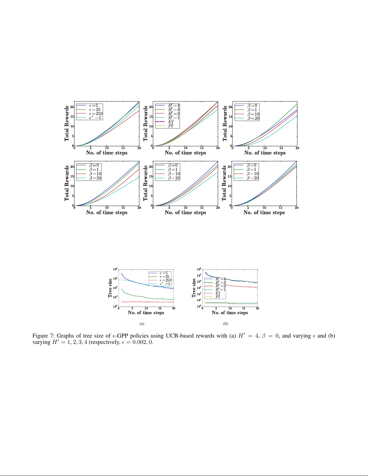
Gaussian Pr ocess Planning with Lipschitz Continuous Reward Functions: T owards Unifying Bay esian Optimization, Activ e Lear ning, and Bey ond Chun Kai Ling ∗ and Kian Hsiang Low ∗ and Patrick J aillet † Department of Computer Science, National Univ ersity of Singapore, Republic of Singapore ∗ Department of Electrical Engineering and Computer Science, Massachusetts Institute of T echnology , USA † { chunkai, lowkh } @comp.nus.edu.sg ∗ , jaillet@mit.edu † Abstract This paper presents a nov el nonmyopic adaptive Gaus- sian pr ocess planning (GPP) framew ork endowed with a general class of Lipschitz continuous rew ard func- tions that can unify some activ e learning/sensing and Bayesian optimization criteria and offer practition- ers some flexibility to specify their desired choices for defining ne w tasks/problems. In particular, it uti- lizes a principled Bayesian sequential decision prob- lem framew ork for jointly and naturally optimizing the exploration-e xploitation trade-off. In general, the re- sulting induced GPP policy cannot be deri ved exactly due to an uncountable set of candidate observations. A key contribution of our work here thus lies in ex- ploiting the Lipschitz continuity of the re ward func- tions to solve for a nonmyopic adaptive  -optimal GPP (  -GPP) policy . T o plan in real time, we further pro- pose an asymptotically optimal, branch-and-bound any- time variant of  -GPP with performance guarantee. W e empirically demonstrate the effecti veness of our  -GPP policy and its anytime variant in Bayesian optimization and an energy harv esting task. 1 Introduction The fundamental challenge of integrated planning and learn- ing is to design an autonomous agent that can plan its ac- tions to maximize its expected total re wards while interact- ing with an unknown task en vironment. Recent research ef- forts tackling this challenge have progressed from the use of simple Markov models assuming discrete-valued, inde- pendent observations (e.g., in Bayesian reinfor cement learn- ing (BRL) (Poupart et al. 2006)) to that of a rich class of Bayesian nonparametric Gaussian pr ocess (GP) models characterizing continuous-valued, correlated observations in order to represent the latent structure of more complex, pos- sibly noisy task en vironments with higher fidelity . Such a challenge is posed by the following important problems in machine learning, among others: Active learning/sensing (AL). In the context of en viron- mental sensing (e.g., adaptiv e sampling in oceanography (Leonard et al. 2007), traffic sensing (Chen et al. 2012; Chen, Lo w , and T an 2013; Chen et al. 2015)), its objec- tiv e is to select the most informati ve (possibly noisy) ob- servations for predicting a spatially varying en vironmental field (i.e., task en vironment) modeled by a GP subject to some sampling budget constraints (e.g., number of sensors, energy consumption). The re wards of an AL agent are de- fined based on some formal measure of predictiv e uncer- tainty such as the entrop y or mutual information criterion. T o resolve the issue of sub-optimality (i.e., local maxima) faced by greedy algorithms (Krause, Singh, and Guestrin 2008; Low et al. 2012; Ouyang et al. 2014; Zhang et al. 2016), re- cent dev elopments have made nonmyopic AL computation- ally tractable with provable performance guarantees (Cao, Low , and Dolan 2013; Hoang et al. 2014; Low , Dolan, and Khosla 2009; 2008; 2011), some of which ha v e fur - ther inv estigated the performance adv antage of adaptivity by proposing nonmyopic adaptive observ ation selection poli- cies that depend on past observations. Bayesian optimization (BO). Its objecti v e is to select and gather the most informativ e (possibly noisy) observations for finding the global maximum of an unknown, highly complex (e.g., non-con vex, no closed-form expression nor deriv ative) objectiv e function (i.e., task en vironment) mod- eled by a GP giv en a sampling budget (e.g., number of costly function ev aluations). The re wards of a BO agent are defined using an improv ement-based (Brochu, Cora, and de Freitas 2010) (e.g., pr obability of impr ovement (PI) or expected im- pr ovement (EI) over currently found maximum), entropy- based (Hennig and Schuler 2012; Hern ´ andez-Lobato, Hoff- man, and Ghahramani 2014), or upper confidence bound (UCB) acquisition function (Sriniv as et al. 2010). A limi- tation of most BO algorithms is that they are myopic. T o ov ercome this limitation, approximation algorithms for non- myopic adaptiv e BO (Marchant, Ramos, and Sanner 2014; Osborne, Garnett, and Roberts 2009) have been proposed, but their performances are not theoretically guaranteed. General tasks/problems. In practice, other types of re wards (e.g., logarithmic, unit step functions) need to be specified for an agent to plan and operate ef fecti vely in a given real- world task en vironment (e.g., natural phenomenon like wind or temperature) modeled by a GP , as detailed in Section 2. As shall be elucidated later , similarities in the structure of the above problems moti v ate us to consider whether it is possible to tackle the ov erall challenge by devising a nonmy- opic adaptiv e GP planning framework with a general class of reward functions unifying some AL and BO criteria and affording practitioners some flexibility to specify their de- sired choices for defining new tasks/problems. Such an in- tegrated planning and learning frame work has to address the exploration-exploitation trade-off common to the abov e problems: The agent faces a dilemma between gathering ob- servations to maximize its expected total re wards gi ven its current, possibly imprecise belief of the task environment (exploitation) vs. that to improv e its belief to learn more about the en vironment (e xploration). This paper presents a novel nonmyopic adapti ve Gaussian pr ocess planning (GPP) framework endowed with a gen- eral class of Lipschitz continuous reward functions that can unify some AL and BO criteria (e.g., UCB) discussed earlier and of fer practitioners some flexibility to specify their de- sired choices for defining ne w tasks/problems (Section 2). In particular , it utilizes a principled Bayesian sequential deci- sion problem frame work for jointly and naturally optimizing the exploration-e xploitation trade-of f, consequently allo w- ing planning and learning to be integrated seamlessly and performed simultaneously instead of separately (Deisenroth, Fox, and Rasmussen 2015). In general, the resulting induced GPP policy cannot be deri ved exactly due to an uncount- able set of candidate observ ations. A key contribution of our work here thus lies in e xploiting the Lipschitz continu- ity of the re w ard functions to solve for a nonmyopic adap- tiv e  -optimal GPP (  -GPP) policy given an arbitrarily user - specified loss bound  (Section 3). T o plan in real time, we further propose an asymptotically optimal, branch-and- bound anytime variant of  -GPP with performance guaran- tee. Finally , we empirically ev aluate the performances of our  -GPP policy and its anytime v ariant in BO and an energy harvesting task on simulated and real-world en vironmental fields (Section 4). T o ease exposition, the rest of this paper will be described by assuming the task environment to be an en vironmental field and the agent to be a mobile robot, which coincide with the setup of our experiments. 2 Gaussian Process Planning (GPP) Notations and Preliminaries. Let S be the domain of an en vironmental field corresponding to a set of sampling lo- cations. At time step t > 0 , a robot can deterministically mov e from its pre vious location s t − 1 to visit location s t ∈ A ( s t − 1 ) and observes it by taking a corresponding realized (random) field measurement z t ( Z t ) where A ( s t − 1 ) ⊆ S denotes a finite set of sampling locations reachable from its previous location s t − 1 in a single time step. The state of the robot at its initial starting location s 0 is represented by prior observations/data d 0 , h s 0 , z 0 i available before planning where s 0 and z 0 denote, respecti vely , v ectors comprising lo- cations visited/observed and corresponding field measure- ments taken by the robot prior to planning and s 0 is the last component of s 0 . Similarly , at time step t > 0 , the state of the robot at its current location s t is represented by obser - vations/data d t , h s t , z t i where s t , s 0 ⊕ ( s 1 , · · · s t ) and z t , z 0 ⊕ ( z 1 , · · · z t ) denote, respectively , vectors compris- ing locations visited/observed and corresponding field mea- surements taken by the robot up until time step t and ‘ ⊕ ’ denotes vector concatenation. At time step t > 0 , the robot also receiv es a re ward R ( z t , s t ) to be defined later . Modeling Envir onmental Fields with Gaussian Processes (GPs). The GP can be used to model a spatially varying en- vironmental field as follo ws: The field is assumed to be a re- alization of a GP . Each location s ∈ S is associated with a la- tent field measurement Y s . Let Y S , { Y s } s ∈S denote a GP , that is, ev ery finite subset of Y S has a multiv ariate Gaussian distribution (Rasmussen and W illiams 2006). Then, the GP is fully specified by its prior mean µ s , E [ Y s ] and co v ari- ance k ss 0 , cov [ Y s , Y s 0 ] for all s, s 0 ∈ S , the latter of which characterizes the spatial correlation structure of the en viron- ment field and can be defined using a cov ariance function. A common choice is the squared exponential cov ariance func- tion k ss 0 , σ 2 y exp {− 0 . 5( s − s 0 ) > M − 2 ( s − s 0 ) } where σ 2 y is the signal v ariance controlling the intensity of measurements and M is a diagonal matrix with length-scale components l 1 and l 2 gov erning the degree of spatial correlation or “sim- ilarity” between measurements in the respectiv e horizontal and vertical directions of the 2 D fields in our e xperiments. The field measurements taken by the robot are assumed to be corrupted by Gaussian white noise, i.e., Z t , Y s t + ε where ε ∼ N (0 , σ 2 n ) and σ 2 n is the noise v ariance. Suppos- ing the robot has gathered observations d t = h s t , z t i from time steps 0 to t , the GP model can perform probabilistic re- gression by using d t to predict the noisy measurement at any unobserved location s t +1 ∈ A ( s t ) as well as pro vide its pre- dictiv e uncertainty using a Gaussian predicti v e distribution p ( z t +1 | d t , s t +1 ) = N ( µ s t +1 | d t , σ 2 s t +1 | s t ) with the follo wing posterior mean and variance, respecti vely: µ s t +1 | d t , µ s t +1 + Σ s t +1 s t Γ − 1 s t s t ( z t − µ s t ) > σ 2 s t +1 | s t , k s t +1 s t +1 + σ 2 n − Σ s t +1 s t Γ − 1 s t s t Σ s t s t +1 where µ s t is a row vector with mean components µ s for ev- ery location s of s t , Σ s t +1 s t is a row vector with cov ariance components k s t +1 s for every location s of s t , Σ s t s t +1 is the transpose of Σ s t +1 s t , and Γ s t s t , Σ s t s t + σ 2 n I such that Σ s t s t is a cov ariance matrix with components k ss 0 for e very pair of locations s, s 0 of s t . An important property of the GP model is that, unlike µ s t +1 | d t , σ 2 s t +1 | s t is independent of z t . Problem Formulation. T o frame nonmyopic adapti ve Gaussian process planning (GPP) as a Bayesian sequential decision problem, let an adaptiv e policy π be defined to se- quentially decide the next location π ( d t ) ∈ A ( s t ) to be ob- served at each time step t using observations d t ov er a finite planning horizon of H time steps/stages (i.e., sampling bud- get of H locations). The v alue V π 0 ( d 0 ) under an adaptiv e policy π is defined to be the e xpected total rewards achieved by its selected observ ations when starting with some prior observations d 0 and following π thereafter and can be com- puted using the following H -stage Bellman equations: V π t ( d t ) , Q π t ( d t , π ( d t )) Q π t ( d t , s t +1 ) , E [ R ( Z t +1 , s t +1 ) + V π t +1 ( h s t +1 , z t ⊕ Z t +1 i ) | d t , s t +1 ] for stages t = 0 , . . . , H − 1 where V π H ( d H ) , 0 . T o solve the GPP problem, the notion of Bayes-optimality 1 is exploited for selecting observations to achie ve the lar gest 1 Bayes-optimality has been studied in discrete BRL (Poupart et al. 2006) whose assumptions (Section 1) do not hold in GPP . Con- tinuous BRLs (Dallaire et al. 2009; Ross, Chaib-draa, and Pineau 2008) assume a known parametric form of observation function, possible expected total rew ards with respect to all possi- ble induced sequences of future Gaussian posterior beliefs p ( z t +1 | d t , s t +1 ) for t = 0 , . . . , H − 1 to be discussed next. Formally , this in volv es choosing an adaptive polic y π to maximize V π 0 ( d 0 ) , which we call the GPP policy π ∗ . That is, V ∗ 0 ( d 0 ) , V π ∗ 0 ( d 0 ) = max π V π 0 ( d 0 ) . By plugging π ∗ into V π t ( d t ) and Q π t ( d t , s t +1 ) abov e, V ∗ t ( d t ) , max s t +1 ∈A ( s t ) Q ∗ t ( d t , s t +1 ) Q ∗ t ( d t , s t +1 ) , E [ R ( Z t +1 , s t +1 ) | d t , s t +1 ] + E [ V ∗ t +1 ( h s t +1 , z t ⊕ Z t +1 i ) | d t , s t +1 ] (1) for stages t = 0 , . . . , H − 1 where V ∗ H ( d H ) , 0 . T o see how the GPP policy π ∗ jointly and naturally opti- mizes the e xploration-exploitation trade-off, its selected lo- cation π ∗ ( d t ) = arg max s t +1 ∈A ( s t ) Q ∗ t ( d t , s t +1 ) at each time step t affects both the immediate expected reward E [ R ( Z t +1 , s t ⊕ π ∗ ( d t )) | d t , π ∗ ( d t )] giv en current belief p ( z t +1 | d t , π ∗ ( d t )) (i.e., exploitation) as well as the Gaussian posterior belief p ( z t +2 |h s t ⊕ π ∗ ( d t ) , z t ⊕ z t +1 i , π ∗ ( h s t ⊕ π ∗ ( d t ) , z t ⊕ z t +1 i )) at next time step t + 1 (i.e., e xplo- ration), the latter of which influences expected future re- wards E [ V ∗ t +1 ( h s t ⊕ π ∗ ( d t ) , z t ⊕ Z t +1 i ) | d t , π ∗ ( d t )] . In general, the GPP polic y π ∗ cannot be deri ved exactly because the expectation terms in (1) usually cannot be ev al- uated in closed form due to an uncountable set of candidate measurements (Section 1) except for degenerate cases like R ( z t +1 , s t +1 ) being independent of z t +1 and H ≤ 2 . T o ov ercome this dif ficulty , we will show in Section 3 later ho w the Lipschitz continuity of the rew ard functions can be ex- ploited for theoretically guaranteeing the performance of our proposed nonmyopic adapti v e  -optimal GPP polic y , that is, the expected total rewards achiev ed by its selected observ a- tions closely approximates that of π ∗ within an arbitrarily user-specified loss bound  > 0 . Lipschitz Continuous Reward Functions. R ( z t , s t ) , R 1 ( z t ) + R 2 ( z t ) + R 3 ( s t ) where R 1 , R 2 , and R 3 are user-de- fined reward functions that satisfy the conditions below: • R 1 ( z t ) is Lipschitz continuous in z t with Lipschitz con- stant  1 . So, h σ ( u ) , ( R 1 ∗ N (0 , σ 2 ))( u ) is Lipschitz continuous in u with  1 where ‘ ∗ ’ denotes con v olution; • R 2 ( z t ) : Define g σ ( u ) , ( R 2 ∗ N (0 , σ 2 ))( u ) such that (a) g σ ( u ) is well-defined for all u ∈ R , (b) g σ ( u ) can be ev aluated in closed form or computed up to an arbitrary precision in reasonable time for all u ∈ R , and (c) g σ ( u ) is Lipschitz continuous 2 in u with Lipschitz constant  2 ( σ ) ; • R 3 ( s t ) only depends on locations s t visited/observed by the robot up until time step t and is independent of real- ized measurement z t . It can be used to represent some sampling or motion costs or explicitly consider explo- ration by defining it as a function of σ 2 s t +1 | s t . Using the above definition of R ( z t , s t ) , the immediate ex- pected rew ard in (1) ev aluates to E [ R ( Z t +1 , s t +1 ) | d t , s t +1 ] the re ward function to be independent of measurements and past states, and/or , when exploiting GP , maximum lik elihood observa- tions during planning with no prov able performance guarantee. 2 Unlike R 1 , R 2 does not need to be Lipschitz continuous (or continuous); it must only be Lipschitz continuous after con volution with any Gaussian kernel. An e xample of R 2 is unit step function. = ( h σ s t +1 | s t + g σ s t +1 | s t )  µ s t +1 | d t  + R 3 ( s t +1 ) which is Lip- schitz continuous in the realized measurements z t : Lemma 1 Let α ( s t +1 ) , k Σ s t +1 s t Γ − 1 s t s t k and d 0 t , h s t , z 0 t i . Then, | E [ R ( Z t +1 , s t +1 ) | d t ,s t +1 ] − E [ R ( Z t +1 , s t +1 ) | d 0 t ,s t +1 ] | ≤ α ( s t +1 )   1 +  2 ( σ s t +1 | s t )  k z t − z 0 t k . Its proof is in Appendix A. Lemma 1 will be used to prove the Lipschitz continuity of V ∗ t in (1) later . Before doing this, let us consider ho w the Lipschitz continuous re ward functions defined above can unify some AL and BO cri- teria discussed in Section 1 and be used for defining ne w tasks/problems. Active learning/sensing (AL). Setting R ( z t +1 , s t +1 ) = R 3 ( s t +1 ) = 0 . 5 log(2 π eσ 2 s t +1 | s t ) yields the well-known nonmyopic AL al gorithm called maximum entropy sampling (MES) (Shewry and W ynn 1987) which plans/decides loca- tions with maximum entropy to be observed that minimize the posterior entropy remaining in the unobserved areas of the field. Since R ( z t +1 , s t +1 ) is independent of z t +1 , the expectations in (1) go away , thus making MES non-adapti ve and hence a straightforward search algorithm not plagued by the issue of uncountable set of candidate measurements. As such, we will not focus on such a degenerate case. This degenerac y vanishes when the en vironment field is instead a realization of log-Gaussian process. Then, MES becomes adaptiv e (Lo w , Dolan, and Khosla 2009) and its reward function can be represented by our Lipschitz continuous re- ward functions: By setting R 1 ( z t +1 ) = 0 , R 2 and g σ s t +1 | s t as identity functions with  2 ( σ s t +1 | s t ) = 1 , and R 3 ( s t +1 ) = 0 . 5 log(2 π eσ 2 s t +1 | s t ) , E [ R ( Z t +1 , s t +1 ) | d t , s t +1 ] = µ s t +1 | d t + 0 . 5 log(2 π eσ 2 s t +1 | s t ) . Bayesian optimization (BO). The greedy BO algorithm of Sriniv as et al. (2010) utilizes the UCB selection crite- rion µ s t +1 | d t + β σ s t +1 | s t ( β ≥ 0 ) to approximately opti- mize the global BO objective of total field measurements P H t =1 z t taken by the robot or , equiv alently , minimize its to- tal regret. UCB can be represented by our Lipschitz con- tinuous re ward functions: By setting R 1 ( z t +1 ) = 0 , R 2 and g σ s t +1 | s t as identity functions with  2 ( σ s t +1 | s t ) = 1 , and R 3 ( s t +1 ) = β σ s t +1 | s t , E [ R ( Z t +1 , s t +1 ) | d t , s t +1 ] = µ s t +1 | d t + β σ s t +1 | s t . In particular , when β = 0 , it can be deriv ed that our GPP policy π ∗ maximizes the expected to- tal field measurements taken by the robot, hence optimizing the exact global BO objecti ve of Sriniv as et al. (2010) in the expected sense. So, unlike greedy UCB, our nonmyopic GPP framework does not have to explicitly consider an ad- ditional weighted exploration term (i.e., β σ s t +1 | s t ) in its re- ward function because it can jointly and naturally optimize the exploration-e xploitation trade-off, as explained earlier . Nev ertheless, if a stronger exploration beha vior is desired (e.g., in online planning), then β has to be fine-tuned. Dif- ferent from nonmyopic BO algorithm of Marchant, Ramos, and Sanner (2014) using UCB-based rew ards, our proposed nonmyopic  -optimal GPP policy (Section 3) does not need to impose an extreme assumption of maximum likelihood observations during planning and, more importantly , pro- vides a performance guarantee, including for the extreme assumption made by nonmyopic UCB. Our GPP framew ork differs from nonmyopic BO algorithm of Osborne, Garnett, and Roberts (2009) in that e very selected observ ation con- tributes to the total field measurements taken by the robot instead of considering just the e xpected improvement for the last observation. So, it usually does not ha ve to expend all the giv en sampling b udget to find the global maximum. General tasks/problems. In practice, the necessary reward function can be more comple x than the ones specified above that are formed from an identity function of the field mea- surement. For example, consider the problem of placing wind turbines in optimal locations to maximize the total power production. Though the av erage wind speed in a re- gion can be modeled by a GP , the po wer output is not a linear function of the steady-state wind speed. In fact, power pro- duction requires a certain minimum speed kno wn as the cut- in speed. After this threshold is met, po wer output increases and e v entually plateaus. Assuming the cut-in speed is 1 , this effect can be modeled with a logarithmic re ward function 3 : R ( z t +1 , s t +1 ) = R 1 ( z t +1 ) gi v es a value of log( z t +1 ) if z t +1 > 1 , and 0 otherwise where  1 = 1 . T o the best of our knowledge, h σ s t +1 | s t ( u ) has no closed-form expression. In Appendix B, we present other interesting reward functions like unit step function 2 and Gaussian distribution that can be represented by R ( z t +1 , s t +1 ) and used in real-world tasks. Theorem 1 belo w re v eals that V ∗ t ( d t ) (1) with Lipschitz continuous re ward functions is Lipschitz continuous in z t with Lipschitz constant L t ( s t ) defined belo w: Definition 1 Let L H ( s H ) , 0 . F or t = 0 , . . . , H − 1 , de- fine L t ( s t ) , max s t +1 ∈A ( s t ) α ( s t +1 )   1 +  2 ( σ s t +1 | s t )  + L t +1 ( s t +1 ) p 1 + α ( s t +1 ) 2 . Theorem 1 (Lipschitz Continuity of V ∗ t ) F or t = 0 , . . . , H , | V ∗ t ( d t ) − V ∗ t ( d 0 t ) | ≤ L t ( s t ) k z t − z 0 t k . Its proof uses Lemma 1 and is in Appendix C. The result below is a direct consequence of Theorem 1 and will be used to theoretically guarantee the performance of our proposed nonmyopic adaptiv e  -optimal GPP polic y in Section 3: Corollary 1 F or t = 0 , . . . , H , | V ∗ t ( h s t , z t − 1 ⊕ z t i ) − V ∗ t ( h s t , z t − 1 ⊕ z 0 t i ) | ≤ L t ( s t ) | z t − z 0 t | . 3  -Optimal GPP (  -GPP) The k ey idea of constructing our proposed nonmyopic adap- tiv e  -GPP policy is to approximate the e xpectation terms in (1) at every stage using a form of deterministic sampling, as illustrated in the figure below . Specifically , the measure- ment space of p ( z t +1 | d t , s t +1 ) is first partitioned into n ≥ 2 intervals ζ 0 , . . . , ζ n − 1 such that interv als ζ 1 , . . . , ζ n − 2 are equally spaced within the bounded gray region [ µ s t +1 | d t − τ σ s t +1 | s t , µ s t +1 | d t + τ σ s t +1 | s t ] specified by a user-defined width parameter τ ≥ 0 while interv als ζ 0 and ζ n − 1 span the two infinitely long red tails. Note that τ > 0 requires n > 2 for the partition to be v alid. The n sample measurements z 0 . . . z n − 1 are then selected by setting z 0 as upper limit of red interv al ζ 0 , z n − 1 as lower limit of red interval ζ n − 1 , and z 1 , . . . , z n − 2 as centers of the respecti ve gray interv als 3 In reality , the speed-po wer relationship is not exactly log arith- mic, but this approximation suf fices for the purpose of modeling. p ( z t +1 | d t , s t +1 ) z 0 , µ s t +1 | d t − τ σ s t +1 | s t ; z n − 1 , µ s t +1 | d t + τ σ s t +1 | s t ; z i , z 0 + i − 0 . 5 n − 2 ( z n − 1 − z 0 ) for i = 1 , . . . , n − 2 . w i , Φ( 2 iτ n − 2 − τ ) − Φ( 2( i − 1) τ n − 2 − τ ) for i = 1 , . . . , n − 2; w 0 = w n − 1 , Φ( − τ ) . z 0 w 0 z 1 w 1 . . . . . . . . . . . . z i - 1 w i - 1 z i w i z i + 1 w i + 1 z n - 1 w n - 1 z n - 2 w n - 2 . . . . . . . . . . . . z t +1 ζ 1 ζ i - 1 ζ i ζ i + 1 ζ n - 2 ζ 0 ζ n - 1 ζ 1 , . . . , ζ n − 2 . Next, the weights w 0 . . . w n − 1 for the cor- responding sample measurements z 0 , . . . , z n − 1 are defined as the areas under their respective intervals ζ 0 , . . . , ζ n − 1 of the Gaussian predictiv e distribution p ( z t +1 | d t , s t +1 ) . So, P n − 1 i =0 w i = 1 . An example of such a partition is giv en in Appendix D. The selected sample measurements and their corresponding weights can be exploited for approximating V ∗ t with Lipschitz continuous reward functions (1) using the following H -stage Bellman equations: V  t ( d t ) , max s t +1 ∈A ( s t ) Q  t ( d t , s t +1 ) Q  t ( d t , s t +1 ) , g σ s t +1 | s t  µ s t +1 | d t  + R 3 ( s t +1 ) + n − 1 X i =0 w i  R 1 ( z i ) + V  t +1 ( h s t +1 , z t ⊕ z i i )  (2) for stages t = 0 , . . . , H − 1 where V  H ( d H ) , 0 . The result- ing induced  -GPP polic y π  jointly and naturally optimizes the exploration-e xploitation trade-off in a similar manner as that of the GPP policy π ∗ , as explained in Section 2. It is interesting to note that setting τ = 0 yields z 0 = . . . = z n − 1 = µ s t +1 | d t , which is equiv alent to selecting a single sample measurement of µ s t +1 | d t with corresponding weight of 1 . This is identical to the special case of maximum lik eli- hood observations during planning which is the extreme as- sumption used by nonmyopic UCB (Marchant, Ramos, and Sanner 2014) for sampling to gain time ef ficiency . Perf ormance Guarantee. The difficulty in theoretically guaranteeing the performance of our  -GPP policy π  (i.e., relativ e to that of GPP polic y π ∗ ) lies in analyzing how the values of the width parameter τ and deterministic sampling size n can be chosen to satisfy the user-specified loss bound  , as discussed below . The first step is to prove that V  t in (2) approximates V ∗ t in (1) closely for some chosen τ and n v alues, which relies on the Lipschitz continuity of V ∗ t in Corollary 1. Define Λ( n, τ ) to be equal to the value of p 2 /π if n ≥ 2 ∧ τ = 0 , and v alue of κ ( τ ) + η ( n, τ ) if n > 2 ∧ τ > 0 where κ ( τ ) , p 2 /π exp( − 0 . 5 τ 2 ) − 2 τ Φ( − τ ) , η ( n, τ ) , 2 τ (0 . 5 − Φ( − τ )) / ( n − 2) , and Φ is a standard normal CDF . Theorem 2 Suppose that λ > 0 is given. F or all d t and t = 0 , . . . , H , if λ ≥ Λ( n, τ ) σ s t +1 | s t (  1 + L t +1 ( s t +1 )) (3) for all s t +1 ∈ A ( s t ) , then | V  t ( d t ) − V ∗ t ( d t ) | ≤ λ ( H − t ) . Its proof uses Corollary 1 and is giv en in Appendix E. Remark 1 . From Theorem 2, a tighter bound on the error | V  t ( d t ) − V ∗ t ( d t ) | can be achiev ed by decreasing the sam- pling budget of H locations 4 and increasing the determinis- tic sampling size n ; increasing n reduces η ( n, τ ) and hence Λ( n, τ ) , which allo ws λ to be reduced as well. The width parameter τ has a mixed effect on this error bound: Note that κ ( τ ) ( η ( n, τ ) ) is proportional to some upper bound on the error incurred by the extreme sample measurements z 0 and z n − 1 ( z 1 , . . . , z n − 2 ), as shown in Appendix E. Increas- ing τ reduces κ ( τ ) but unfortunately raises η ( n, τ ) . So, in order to reduce Λ( n, τ ) further by increasing τ , it has to be complemented by raising n fast enough to keep η ( n, τ ) from increasing. This allows λ to be reduced further as well. Remark 2 . A feasible choice of τ and n satisfying (3) can be expressed analytically in terms of the given λ and hence computed prior to planning, as shown in Appendix F. Remark 3 . σ s t +1 | s t and L t +1 ( s t +1 ) for all s t +1 and t = 0 , . . . , H − 1 can be computed prior to planning as they de- pend on s 0 and all reachable locations from s 0 but not on their measurements. Using Theorem 2, the next step is to bound the perfor- mance loss of our  -GPP policy π  relativ e to that of GPP policy π ∗ , that is, policy π  is  -optimal: Theorem 3 Given the user-specified loss bound  > 0 , V ∗ 0 ( d 0 ) − V π  0 ( d 0 ) ≤  by substituting λ = / ( H ( H + 1)) into the choice of τ and n stated in Remark 2 above . Its proof is in Appendix G. It can be observed from Theo- rem 3 that a tighter bound  on the error V ∗ 0 ( d 0 ) − V π  0 ( d 0 ) can be achie ved by decreasing the sampling budget of H locations 4 and increasing the deterministic sampling size n . The effect of width parameter τ on this error bound  is the same as that on the error bound of | V  t ( d t ) − V ∗ t ( d t ) | , as explained in Remark 1 above. Anytime  -GPP . Unlike GPP policy π ∗ , our  -GPP policy π  can be deriv ed e xactly since its incurred time is indepen- dent of the size of the uncountable set of candidate measure- ments. Howe ver , e xpanding the entire search tree of  -GPP (2) incurs time containing a O ( n H ) term and is not always necessary to achiev e  -optimality in practice. T o mitigate this computational difficulty 5 , we propose an anytime v ari- ant of  -GPP that can produce a good policy fast and improv e its approximation quality over time, as briefly discussed here and detailed with the pseudocode in Appendix H. The key intuition is to expand the sub-trees rooted at “promising” nodes with the highest weighted uncertainty of their corresponding v alues V ∗ t ( d t ) so as to impro v e their es- timates. T o represent such uncertainty at each encountered node, upper & lower heuristic bounds (respectiv ely , V ∗ t ( d t ) and V ∗ t ( d t ) ) are maintained, like in (Smith and Simmons 2006). A partial construction of the entire tree is maintained and e xpanded incrementally in each iteration of anytime  - GPP that incurs linear time in n and comprises 3 steps: Node selection. T raverse down the partially constructed tree by repeatedly selecting nodes with largest difference be- tween their upper and lower bounds (i.e., uncertainty) dis- counted by weight w i ∗ of its preceding sample measurement 4 This changes  -GPP by reducing its planning horizon though. 5 The value of n is a bigger computational issue than that of H when  is small and in online planning. z i ∗ until an unexpanded node, denoted by d t , is reached. Expand tree. Construct a “minimal” sub-tree rooted at node d t by sampling all possible ne xt locations and only their me- dian sample measurements z ¯ i recursiv ely up to full height H . Backpropagation. Backpropagate bounds from the leav es of the newly constructed sub-tree to node d t , during which the refined bounds of expanded nodes are used to inform the bounds of unexpanded siblings by exploiting the Lip- schitz continuity of V ∗ t (Corollary 1), as explained in Ap- pendix H. Backpropagate bounds to the root of the partially constructed tree in a similar manner . By using the lower heuristic bound to produce our any- time  -GPP policy , its performance loss relati ve to that of GPP policy π ∗ can be bounded, as prov en in Appendix H. 4 Experiments and Discussion This section empirically ev aluates the online planning per- formance and time ef ficienc y of our  -GPP policy π  and its anytime v ariant under limited sampling budget in an energy harvesting task on a simulated wind speed field and in BO on simulated plankton density (chl-a) field and real-world log- potassium (lg-K) concentration (mg l − 1 ) field (Appendix I) of Broom’ s Barn farm (W ebster and Oli v er 2007). Each sim- ulated (real-world lg-K) field is spatially distributed ov er a 0 . 95 km by 0 . 95 km ( 520 m by 440 m) region discretized into a 20 × 20 ( 14 × 12 ) grid of sampling locations. These fields are assumed to be realizations of GPs. The wind speed (chl-a) field is simulated using hyperparameters µ s = 0 , 6 l 1 = l 2 = 0 . 2236 ( 0 . 2 ) km, σ 2 n = 10 − 5 , and σ 2 y = 1 . The hyperparameters µ s = 3 . 26 , l 1 = 42 . 8 m, l 2 = 103 . 6 m, σ 2 n = 0 . 0222 , and σ 2 y = 0 . 057 of lg-K field are learned using maximum likelihood estimation (Rasmussen and Williams 2006). The robot’ s initial starting location is near to the cen- ter of each simulated field and randomly selected for lg-K field. It can move to any of its 4 adjacent grid locations at each time step and is tasked to maximize its total rew ards ov er 20 time steps (i.e., sampling budget of 20 locations). In BO, the performances of our  -GPP polic y π  and its anytime v ariant are compared with that of state-of-the-art nonmyopic UCB (Marchant, Ramos, and Sanner 2014) and gr eedy PI, EI, UCB (Brochu, Cora, and de Freitas 2010; Sriniv as et al. 2010). Three performance metrics are used: (a) T otal rewards achieved ov er the evolv ed time steps (i.e., higher total rewards imply less total regret in BO (Sec- tion 2)), (b) maximum re w ard achie v ed during experiment, and (c) search tree size in terms of no. of nodes (i.e., lar ger tree size implies higher incurred time). All e xperiments are run on a Linux machine with Intel Core i 5 at 1 . 7 GHz. Energy Harvesting T ask on Simulated Wind Speed Field. A robotic rover equipped with a wind turbine is tasked to harvest energy/po wer from the wind while e xploring a polar region (Chen et al. 2014). It is driv en by the logarithmic re- ward function described under ‘General tasks/problems’ in Section 2. Fig. 1 shows results of performances of our  -GPP policy and its anytime variant av eraged over 30 indepen- dent realizations of the wind speed field. It can be observed 6 Its actual prior mean is not zero; we ha ve applied zero-mean GP to Y s − µ s for simplicity . Figure 1: Graphs of total re wards and tree size of  -GPP policies with (a-b) online planning horizon H 0 = 4 and varying  and (c-d) varying H 0 = 1 , 2 , 3 , 4 (respectiv ely ,  = 0 . 002 , 0 . 06 , 0 . 8 , 5 ) (a) (b) (c) (d) vs. no. of time steps for energy harvesting task. The plot of  ∗ = 5 uses our an ytime v ariant with a maximum tree size of 5 × 10 4 nodes while the plot of  = 250 ef fecti v ely assumes maximum likelihood observations during planning lik e that of nonmyopic UCB (Marchant, Ramos, and Sanner 2014). that the gradients of the achie v ed total rewards (i.e., power production) increase over time, which indicate a higher ob- tained reward with an increasing number of time steps as the robot can exploit the environment more effecti vely with the aid of exploration from pre vious time steps. The gradients ev entually stop increasing when the robot enters a perceiv ed high-rew ard region. Further exploration is deemed unnec- essary as it is unlikely to find another preferable location within H 0 time steps; so, the robot remains near-stationary for the remaining time steps. It can also be observed that the incurred time is much higher in the first few time steps. This is expected because the posterior v ariance σ s t +1 | s t decreases with increasing time step t , thus requiring a decreasing de- terministic sampling size n to satisfy (3). Initially , all  -GPP policies achieve similar total rew ards as the robots begin from the same starting location. After some time,  -GPP policies with lower user-specified loss bound  and longer online planning horizon H 0 achiev e con- siderably higher total rewards at the cost of more incurred time. In particular , it can be observed that a robot assum- ing maximum likelihood observations during planning (i.e.,  = 250 ) like that of nonmyopic UCB or using a greedy policy (i.e., H 0 = 1 ) performs poorly very quickly . In the former case (Fig. 1a), the gradient of its total rewards stops increasing quite early (i.e., from time step 9 onwards), which indicates that its perceived local maximum is reached pre- maturely . Interestingly , it can be observed from Fig. 1d that the  -GPP policy with H 0 = 2 and  = 0 . 06 incurs more time than that with H 0 = 3 and  = 0 . 8 despite the lat- ter achieving higher total rew ards. This suggests trading off tighter loss bound  for longer online planning horizon H 0 , especially when  is too small that in turn requires a very large n and consequently incurs significantly more time 5 . BO on Real-W orld Log-Potassium Concentration Field. An agricultural robot is tasked to find the peak lg-K mea- surement (i.e., possibly in an o ver -fertilized area) while e x- ploring the Broom’ s Barn farm (W ebster and Oli ver 2007). It is driv en by the UCB-based re w ard function described under ‘BO’ in Section 2. Fig. 2 shows results of performances of our  -GPP policy and its anytime variant, nonmyopic UCB (i.e.,  = 25 ), and greedy PI, EI, UCB (i.e., H 0 = 1 ) av er - (a) (b) (c) Figure 2: Graphs of total normalized 7 rew ards of  -GPP poli- cies using UCB-based re wards with (a) H 0 = 4 , β = 0 , and varying  , (b) v arying H 0 = 1 , 2 , 3 , 4 (respectively ,  = 0 . 002 , 0 . 003 , 0 . 4 , 2 ) and β = 0 , and (c) H 0 = 4 ,  = 1 , and varying β vs. no. of time steps for BO on real-world lg- K field. The plot of  ∗ = 1 uses our an ytime variant with a maximum tree size of 3 × 10 4 nodes while the plot of  = 25 effecti vely assumes maximum likelihood observations dur- ing planning like that of nonmyopic UCB. aged over 25 randomly selected robot’ s initial starting lo- cation. It can be observed from Figs. 2a and 2b that the gradients of the achiev ed total normalized 7 rew ards gener- ally increase ov er time. In particular , from Fig. 2a, nonmy- opic UCB assuming maximum likelihood observations dur- ing planning obtains much less total rewards than the other  - GPP policies and the an ytime v ariant after 20 time steps and finds a maximum lg-K measurement of 3 . 62 that is at least 0 . 4 σ y worse after 20 time steps. The performance of the any- time variant is comparable to that of our best-performing  - GPP policy with  = 3 . From Fig. 2b, the greedy policy (i.e., H 0 = 1 ) with β = 0 performs much more poorly than its nonmyopic  -GPP counterparts and finds a maximum lg-K measurement of 3 . 56 that is lo wer than that of greedy PI and EI due to its lack of exploration. By increasing H 0 to 2 - 4 , our  -GPP policies with β = 0 outperform greedy PI and EI as they can naturally and jointly optimize the exploration- exploitation trade-off. Interestingly , Fig. 2c shows that our  -GPP policy with β = 2 achie ves the highest total rew ards after 20 time steps, which indicates the need of a slightly stronger exploration behavior than that with β = 0 . This may be e xplained by a small length-scale (i.e., spatial corre- lation) of the lg-K field, thus requiring some exploration to find the peak measurement. By increasing H 0 beyond 4 or with larger spatial correlation (Appendix J), we expect a di- minishing role of the β σ s t +1 | s t term. It can also be observ ed that aggressiv e exploration (i.e., β ≥ 10 ) hurts the perfor- mance. Results of the tree size (i.e., incurred time) of our  -GPP policy and its an ytime v ariant are in Appendix I. Due to lack of space, we present additional e xperimental results for BO on simulated plankton density field in Ap- pendix J that yield similar observations to the abo v e. 5 Conclusion This paper describes a nov el nonmyopic adapti ve  -GPP framew ork endo wed with a general class of Lipschitz con- tinuous rew ard functions that can unify some AL and BO criteria and be used for defining new tasks/problems. In par - ticular , it can jointly and naturally optimize the exploration- exploitation trade-off. W e theoretically guarantee the perfor- mances of our  -GPP policy and its anytime variant and em- 7 T o ease interpretation of the results, each rew ard is normalized by subtracting the prior mean from it. pirically demonstrate their ef fecti veness in BO and an en- ergy harvesting task. For our future work, we plan to scale up  -GPP and its anytime variant for big data using paral- lelization (Chen et al. 2013; Low et al. 2015), online learn- ing (Xu et al. 2014), and stochastic variational inference (Hoang, Hoang, and Low 2015) and extend them to handle unknown h yperparameters (Hoang et al. 2014). Acknowledgments. This work was supported by Singapore- MIT Alliance for Research and T echnology Subaward Agreement No. 52 R- 252 - 000 - 550 - 592 . References Brochu, E.; Cora, V . M.; and de Freitas, N. 2010. A tuto- rial on Bayesian optimization of expensi v e cost functions, with application to activ e user modeling and hierarchical re- inforcement learning. Cao, N.; Low , K. H.; and Dolan, J. M. 2013. Multi-robot in- formativ e path planning for activ e sensing of en vironmental phenomena: A tale of two algorithms. In Pr oc. AAMAS . Chen, J.; Lo w , K. H.; T an, C. K.-Y .; Oran, A.; Jaillet, P .; Dolan, J. M.; and Sukhatme, G. S. 2012. Decentralized data fusion and active sensing with mobile sensors for modeling and predicting spatiotemporal traffic phenomena. In Proc. U AI , 163–173. Chen, J.; Cao, N.; Low , K. H.; Ouyang, R.; T an, C. K.-Y .; and Jaillet, P . 2013. Parallel Gaussian process regression with low-rank covariance matrix approximations. In Pr oc. U AI , 152–161. Chen, J.; Liang, J.; W ang, T .; Zhang, T .; and W u, Y . 2014. Design and power management of a wind-solar-powered po- lar rov er . Journal of Ocean and W ind Ener gy 1(2):65–73. Chen, J.; Lo w , K. H.; Jaillet, P .; and Y ao, Y . 2015. Gaussian process decentralized data fusion and acti ve sensing for spa- tiotemporal traf fic modeling and prediction in mobility-on- demand systems. IEEE T rans. Autom. Sci. Eng. 12:901–921. Chen, J.; Low , K. H.; and T an, C. K.-Y . 2013. Gaussian process-based decentralized data fusion and acti ve sensing for mobility-on-demand system. In Pr oc. RSS . Dallaire, P .; Besse, C.; Ross, S.; and Chaib-draa, B. 2009. Bayesian reinforcement learning in continuous POMDPs with Gaussian processes. In Pr oc. IEEE/RSJ IR OS , 2604– 2609. Deisenroth, M. P .; Fox, D.; and Rasmussen, C. E. 2015. Gaussian processes for data-efficient learning in robotics and control. IEEE T ransactions on P attern Analysis and Ma- chine Intelligence 37(2):408–423. Dolan, J. M.; Podnar , G.; Stanclif f, S.; Low , K. H.; Elfes, A.; Higinbotham, J.; Hosler, J. C.; Moisan, T . A.; and Moisan, J. 2009. Cooperative aquatic sensing using the telesuper- vised adapti ve ocean sensor fleet. In Pr oc. SPIE Conference on Remote Sensing of the Ocean, Sea Ice, and Large W ater Re gions , v olume 7473. Hennig, P ., and Schuler, C. J. 2012. Entropy search for information-efficient global optimization. JMLR 13:1809– 1837. Hern ´ andez-Lobato, J. M.; Hoffman, M. W .; and Ghahra- mani, Z. 2014. Predicti v e entrop y search for efficient global optimization of black-box functions. In Pr oc. NIPS . Hoang, T . N.; Lo w , K. H.; Jaillet, P .; and Kankanhalli, M. 2014. Nonmyopic  -Bayes-optimal activ e learning of Gaus- sian processes. In Pr oc. ICML , 739–747. Hoang, T . N.; Hoang, Q. M.; and Lo w , K. H. 2015. A unifying framework of anytime sparse Gaussian process re- gression models with stochastic variational inference for big data. In Pr oc. ICML , 569–578. Krause, A.; Singh, A.; and Guestrin, C. 2008. Near-optimal sensor placements in Gaussian processes: Theory , efficient algorithms and empirical studies. JMLR 9:235–284. Leonard, N. E.; P alley , D. A.; Lekien, F .; Sepulchre, R.; Fratantoni, D. M.; and Davis, R. E. 2007. Collective motion, sensor networks, and ocean sampling. Pr oc. IEEE 95:48–74. Low , K. H.; Chen, J.; Dolan, J. M.; Chien, S.; and Thomp- son, D. R. 2012. Decentralized active robotic exploration and mapping for probabilistic field classification in en viron- mental sensing. In Pr oc. AAMAS , 105–112. Low , K. H.; Y u, J.; Chen, J.; and Jaillet, P . 2015. Parallel Gaussian process regression for big data: Lo w-rank repre- sentation meets Markov approximation. In Pr oc. AAAI . Low , K. H.; Dolan, J. M.; and Khosla, P . 2008. Adaptiv e multi-robot wide-area exploration and mapping. In Pr oc. AAMAS , 23–30. Low , K. H.; Dolan, J. M.; and Khosla, P . 2009. Information- theoretic approach to ef ficient adaptive path planning for mobile robotic en vironmental sensing. In Proc. ICAPS . Low , K. H.; Dolan, J. M.; and Khosla, P . 2011. Active Markov information-theoretic path planning for robotic en- vironmental sensing. In Pr oc. AAMAS , 753–760. Marchant, R.; Ramos, F .; and Sanner , S. 2014. Sequential Bayesian optimisation for spatial-temporal monitoring. In Pr oc. UAI . Osborne, M. A.; Garnett, R.; and Roberts, S. J. 2009. Gaus- sian processes for global optimization. In Pr oc. 3r d Interna- tional Conference on Learning and Intelligent Optimization . Ouyang, R.; Lo w , K. H.; Chen, J.; and Jaillet, P . 2014. Multi- robot activ e sensing of non-stationary Gaussian process- based en vironmental phenomena. In Proc. AAMAS . Poupart, P .; Vlassis, N.; Hoey , J.; and Re gan, K. 2006. An analytic solution to discrete Bayesian reinforcement learn- ing. In Pr oc. ICML , 697–704. Rasmussen, C. E., and Williams, C. K. I. 2006. Gaussian Pr ocesses for Machine Learning . MIT Press. Ross, S.; Chaib-draa, B.; and Pineau, J. 2008. Bayesian rein- forcement learning in continuous POMDPs with application to robot navigation. In Pr oc. IEEE ICRA , 2845–2851. Shewry , M. C., and W ynn, H. P . 1987. Maximum entropy sampling. J. Applied Statistics 14(2):165–170. Smith, T ., and Simmons, R. 2006. Focused real-time dy- namic programming for MDPs: Squeezing more out of a heuristic. In Pr oc. AAAI , 1227–1232. Sriniv as, N.; Krause, A.; Kakade, S.; and Seeger , M. 2010. Gaussian process optimization in the bandit setting: No re- gret and experimental design. In Proc. ICML , 1015–1022. W ebster, R., and Oliv er , M. 2007. Geostatistics for Envir on- mental Scientists . NY : John W iley & Sons, Inc., 2nd edition. Xu, N.; Low , K. H.; Chen, J.; Lim, K. K.; and Ozgul, E. B. 2014. GP-Localize: Persistent mobile robot localization us- ing online sparse Gaussian process observation model. In Pr oc. AAAI , 2585–2592. Zhang, Y .; Hoang, T . N.; Lo w , K. H.; and Kankanhalli, M. 2016. Near-optimal active learning of multi-output Gaussian processes. In Pr oc. AAAI . A Proof of Lemma 1 Since h σ s t +1 | s t and g σ s t +1 | s t are Lipschitz continuous with the respecti ve Lipschitz constants  1 and  2 ( σ s t +1 | s t ) (Section 2), E [ R ( Z t +1 , s t +1 ) | d t , s t +1 ] is Lipschitz continuous in µ s t +1 | d t with Lipschitz constant  1 +  2 ( σ s t +1 | s t ) . Then, by using the definition of GP posterior mean µ s t +1 | d t and Cauchy-Schwarz inequality , Lemma 1 results. B Other Complex Reward Functions Represented by R When sampling a natural phenomenon, locations featuring a specific band of field measurements may be preferred. Suppose that a robot is task ed to gather algal samples from an aquatic environment. It is well established that algal growth is f aster in certain temperature range and survi v al is not possible at either extremes. The temperature field can be modeled as a GP . A rectangular reward function can be used to direct the robot to search among regions with the specified temperature range. The rectangular reward function can be viewed as a difference of two unit step functions, each of which is of the form: R 2 ( z t +1 ) giv es a v alue of 1 if z t +1 > a , and 0 otherwise where a is some user-defined constant. For such a step function, g σ s t +1 | s t ( u ) = 1 − Φ(( a − u ) /σ s t +1 | s t ) and  2 ( σ s t +1 | s t ) = 1 / ( √ 2 π σ s t +1 | s t ) . Another interesting re w ard function is the Gaussian distrib ution itself 8 which may be represented using R 2 ( z t +1 ) = N (0 , 1) , g σ s t +1 | s t ( u ) = (2 π (1 + σ 2 s t +1 | s t )) − 1 / 2 exp( − u 2 / (2(1 + σ 2 s t +1 | s t ))) and  2 ( σ s t +1 | s t ) = ( √ 2 π (1 + σ 2 s t +1 | s t )) − 1 exp( − 1 / 2) . C Proof of Theor em 1 W e will give a proof by induction on t that | V ∗ t ( d t ) − V ∗ t ( d 0 t ) | ≤ L t ( s t ) k z t − z 0 t k . (4) When t = H , | V ∗ H ( d H ) − V ∗ H ( d 0 H ) | = 0 ≤ L H ( s H ) k z H − z 0 H k . Supposing (4) holds for t + 1 (i.e., induction hypothesis), we will prove that it holds for 0 ≤ t < H . W ithout loss of generality , assume that V ∗ t ( d t ) ≥ V ∗ t ( d 0 t ) . Let s ∗ t +1 , π ∗ ( d t ) and ∆ t +1 , µ s ∗ t +1 | d t − µ s ∗ t +1 | d 0 t . Then, | ∆ t +1 | ≤ α ( s t ⊕ s ∗ t +1 ) k z t − z 0 t k . V ∗ t ( d t ) − V ∗ t ( d 0 t ) ≤ Q ∗ t ( d t , s ∗ t +1 ) − Q ∗ t ( d 0 t , s ∗ t +1 ) = E [ R ( Z t +1 , s t ⊕ s ∗ t +1 ) | d t , s ∗ t +1 ] − E [ R ( Z t +1 , s t ⊕ s ∗ t +1 ) | d 0 t , s ∗ t +1 ] + Z ∞ −∞ p ( z t +1 | d t , s ∗ t +1 ) V ∗ t +1 ( d t +1 ) d z t +1 − Z ∞ −∞ p ( z 0 t +1 | d 0 t , s ∗ t +1 ) V ∗ t +1 ( d 0 t +1 ) d z 0 t +1 ≤ | ∆ t +1 |   1 +  2 ( σ s ∗ t +1 | s t )  + Z ∞ −∞ p ( z t +1 | d t , s ∗ t +1 ) L t +1 ( s t ⊕ s ∗ t +1 ) k ( z t − z 0 t ) ⊕ ∆ t +1 k d z t +1 = | ∆ t +1 |   1 +  2 ( σ s ∗ t +1 | s t )  + L t +1 ( s t ⊕ s ∗ t +1 ) k ( z t − z 0 t ) ⊕ ∆ t +1 k ≤ α ( s t ⊕ s ∗ t +1 ) k z t − z 0 t k   1 +  2 ( σ s ∗ t +1 | s t )  + L t +1 ( s t ⊕ s ∗ t +1 ) q 1 + α ( s t ⊕ s ∗ t +1 ) 2 k z t − z 0 t k =  α ( s t ⊕ s ∗ t +1 )   1 +  2 ( σ s ∗ t +1 | s t )  + L t +1 ( s t ⊕ s ∗ t +1 ) q 1 + α ( s t ⊕ s ∗ t +1 ) 2  k z t − z 0 t k ≤ L t ( s t ) k z t − z 0 t k . The first equality is due to (1). The second inequality follo ws from Lemma 1, change of v ariable z 0 t +1 , z t +1 − ∆ t +1 , and the induction hypothesis. The last inequality is due to definition of L t (Definition 1). 8 Con v olution between two Gaussian distributions yields another Gaussian which is Lipschitz continuous. An alternati ve formulation is to set R 1 ( z t +1 ) = N (0 , 1) since the rew ard function is itself Lipschitz continuous. D Illustration of Deterministic Sampling Strategy p ( z t +1 | d t , s t +1 ) − 5 σ − 4 σ − 3 σ − 2 σ 2 σ 3 σ 4 σ 5 σ − σ 0 σ z t +1 z 0 w 0 z 1 w 1 z 2 w 2 z 3 w 3 z 4 w 4 R 1 ( z t +1 ) + V ∗ t +1 ( h s t +1 , z t ⊕ z t +1 i ) ζ 1 ζ 2 ζ 3 ζ 0 ζ 4 τ σ z t +1 Figure 3: Example of a possible partition with µ s t +1 | d t = 0 , τ = 3 , and n = 5 where we let σ , σ s t +1 | s t for notational simplicity . At the bottom, the measurement space of p ( z t +1 | d t , s t +1 ) is partitioned into 5 interv als ζ 0 , ζ 1 , ζ 2 , ζ 3 , and ζ 4 such that interv als ζ 1 , ζ 2 , and ζ 3 are equally spaced within the bounded gray re gion [ − 3 σ , 3 σ ] while interv als ζ 0 and ζ 4 span the tw o infinitely long red tails. The 5 sample measurements z 0 , z 1 , z 2 , z 3 , and z 4 are then selected by setting z 0 as the upper limit of red interval ζ 0 , z 4 as the lower limit of red interval ζ 4 , and z 1 , z 2 , and z 3 as the centers of the respecti ve gray interv als ζ 1 , ζ 2 , and ζ 3 . The weights w 0 , w 1 , w 2 , w 3 , and w 4 for the corresponding sample measurements z 0 , z 1 , z 2 , z 3 , and z 4 are defined as the areas under their respective intervals ζ 0 , ζ 1 , ζ 2 , ζ 3 , and ζ 4 of the Gaussian predictive distribution p ( z t +1 | d t , s t +1 ) . At the top, the brown curve (i.e., Lipschitz continuous) denotes the sum of R 1 ( z t +1 ) and the expected future re wards V ∗ t +1 ( h s t +1 , z t ⊕ z t +1 i ) achiev ed by the GPP policy . The latter is unknown in practice, as explained in Section 2. The blue curv e sho ws the rectangular approximations using the sample measurements z 0 , z 1 , z 2 , z 3 , and z 4 . Note that, in reality , V ∗ t +1 cannot be accurately e valuated – there will be additional errors accruing from future time steps that are not reflected in this figure b ut will be formally accounted for in the theoretical performance guarantee of our  -GPP policy , as shown in the proof of Theorem 2 in Appendix E. E Proof of Theor em 2 There are tw o sources of error arising in using V  t in (2) to approximate V ∗ t in (1): (a) In our deterministic sampling strate gy (Section 3), only a finite number of sample measurements is selected for approximating the stage-wise expectation terms in (1), and (b) computing V  t does not in v olve utilizing the v alues of V ∗ t +1 but that of its approximation V  t +1 instead. T o facilitate capturing the error due to finite deterministic sampling described in (a), the following intermediate function is introduced: U ∗ t ( d t , s t +1 ) , g σ s t +1 | s t  µ s t +1 | d t  + R 3 ( s t +1 ) + n − 1 X i =0 w i  R 1 ( z i ) + V ∗ t +1 ( h s t +1 , z t ⊕ z i i )  (5) for stages t = 0 , . . . , H − 1 where V ∗ H ( d H ) , 0 . The following lemma bounds the error between U ∗ t and Q ∗ t , which can then be used to bound the error between V  t and V ∗ t : Lemma 2 F or t = 0 , . . . , H − 1 , | U ∗ t ( d t , s t +1 ) − Q ∗ t ( d t , s t +1 ) | ≤ λ . Pr oof . When n > 2 , define ¯ z , z n − 1 − z 0 n − 2 . Then, ζ 0 = [ −∞ , z 0 ] , ζ n − 1 = [ z n − 1 , ∞ ] , and ζ i = [ z 0 + ( i − 1) ¯ z , z 0 + i ¯ z ] for i = 1 , . . . , n − 2 . For i = 0 , . . . , n − 1 , w i = Z z t +1 ∈ ζ i p ( z t +1 | d t , s t +1 ) d z t +1 . Observe that the integration limits form a partition (at least in the sense of a Riemannian integral) of R , thus implying P n − 1 i =0 w i = 1 . | U ∗ t ( d t , s t +1 ) − Q ∗ t ( d t , s t +1 ) | =        n − 1 X i =0 Z ζ i p ( z t +1 | d t , s t +1 )  V ∗ t +1 ( h s t +1 , z t ⊕ z i i ) + R 1 ( z i ) − V ∗ t +1 ( h s t +1 , z t ⊕ z t +1 i ) − R 1 ( z t +1 )  d z t +1        ≤ n − 1 X i =0 Z ζ i p ( z t +1 | d t , s t +1 )   V ∗ t +1 ( h s t +1 , z t ⊕ z i i ) + R 1 ( z i ) − V ∗ t +1 ( h s t +1 , z t ⊕ z t +1 i ) − R 1 ( z t +1 )   d z t +1 ≤ (  1 + L t +1 ( s t +1 )) n − 1 X i =0 Z ζ i p ( z t +1 | d t , s t +1 )   z i − z t +1   d z t +1 . (6) The last inequality follo ws from Corollary 1 and the fact that R 1 is Lipschitz continuous with Lipschitz constant  1 (Section 2). W e now focus on the integral within the summation. When i = 0 , Z ζ 0 p ( z t +1 | d t , s t +1 )   z 0 − z t +1   d z t +1 = σ s t +1 | s t √ 2 π Z − τ −∞ exp  − y 2 2  ( − τ − y ) d y = σ s t +1 | s t  1 √ 2 π exp  − τ 2 2  − τ Φ( − τ )  = 1 2 σ s t +1 | s t κ ( τ ) . (7) The first equality can be obtained by plugging in the density function of a Gaussian and normalizing. A similar result can be obtained when i = n − 1 . When n > 2 , n − 2 X i =1 Z ζ i p ( z t +1 | d t , s t +1 )   z i − z t +1   d z t +1 ≤ ¯ z 2 n − 2 X i =1 Z ζ i p ( z t +1 | d t , s t +1 ) d z t +1 = τ σ s t +1 | s t n − 2 Z n − 2 S i =1 ζ i p ( z t +1 | d t , s t +1 ) d z t +1 = 2 τ σ s t +1 | s t n − 2  1 2 − Φ( − τ )  = σ s t +1 | s t η ( n, τ ) . (8) The inequality is obtained by observing that z i is the center of ζ i for i = 1 , . . . , n − 2 and that each interval ζ i for i = 1 , . . . , n − 2 is of equal length ¯ z . The first equality is obtained by combining the definitions of ¯ z , z 0 , and z n − 1 . Plugging (7) and (8) into (6) giv es | U ∗ t ( d t , s t +1 ) − Q ∗ t ( d t , s t +1 ) | ≤ Λ( n, τ ) σ s t +1 | s t (  1 + L t +1 ( s t +1 )) A similar deriv ation shows that the result is also true when n = 2 . Using (3), Lemma 2 results.  Main Pr oof . W e will give a proof by induction on t that | V  t ( d t ) − V ∗ t ( d t ) | ≤ λ ( H − t ) . (9) The base case of t = H is trivially true. Supposing (9) holds for t + 1 (i.e., induction hypothesis), we will prove that it holds for 0 ≤ t < H . For all s t +1 ∈ A ( s t ) , | Q  t ( d t , s t +1 ) − Q ∗ t ( d t , s t +1 ) | ≤ | Q  t ( d t , s t +1 ) − U ∗ t ( d t , s t +1 ) | + | U ∗ t ( d t , s t +1 ) − Q ∗ t ( d t , s t +1 ) | | {z } ≤ λ ≤ λ + n − 1 X i =0 w i   V  t +1 ( s t +1 , z t ⊕ z i ) − V ∗ t +1 ( s t +1 , z t ⊕ z i )   ≤ λ ( H − t ) . (10) The second inequality follows from Lemma 2 and the definitions of Q  t (2) and U ∗ t . The last inequality follows from the induction hypothesis and the fact that P n − 1 i =0 w i = 1 . Then, | V  t − V ∗ t ( d t ) | ≤      max s t +1 ∈A ( s t ) Q  t ( d t , s t +1 ) − max s 0 t +1 ∈A ( s t ) Q ∗ t ( d t , s 0 t +1 )      ≤ max s t +1 ∈A ( s t ) | Q  t ( d t , s t +1 ) − Q ∗ t ( d t , s t +1 ) | ≤ λ ( H − t ) . The final inequality is due to (10). F Analytically Computing a F easible Choice of τ and n Set n = 2 + τ r π 2 exp  τ 2 2  . (11) Then, Λ( n, τ ) = κ ( τ ) + η ( n, τ ) ≤ r 2 π exp  − τ 2 2  + τ n − 2 = 2 r 2 π exp  − τ 2 2  . Using (3), the feasible values of τ satisfy 2 r 2 π exp  − τ 2 2  ≤ λ σ s t +1 | s t (  1 + L t +1 ( s t +1 )) . So, a feasible choice of τ can be obtained from 2 r 2 π exp  − τ 2 2  = λ σ s t +1 | s t (  1 + L t +1 ( s t +1 )) , which giv es τ = s − 2 log  r π 2 λ 2 σ s t +1 | s t (  1 + L t +1 ( s t +1 ))  . By substituting this value of τ into (11), the value of n can be obtained. If n is not an integer , then take the ceiling of n . If the deterministic sampling size n is to be constrained (i.e., less than some user -defined constant b n ) to preserve the time ef ficiency of solving for the  -GPP policy , then a numerical alternativ e is available: For all n < b n , min τ Λ( n, τ ) can be computed numerically of fline. Choosing the values of τ and n to satisfy (3) simply inv olv es finding n ∗ < b n such that min τ Λ( n ∗ , τ ) ≤ λ/ ( σ s t +1 | s t (  1 + L t +1 ( s t +1 ))) . G Proof of Theor em 3 W e will give a proof by induction on t that V ∗ t ( d t ) − V π  t ( d t ) ≤ λ ( H − t )( H − t + 1) . (12) The base case of t = H is trivially true. Supposing (12) holds for t + 1 (i.e., induction hypothesis), we will prove that it holds for 0 ≤ t < H . For all s t +1 ∈ A ( s t ) , | Q ∗ t ( d t , s t +1 ) − Q π  t ( d t , s t +1 ) | ≤ ∞ Z −∞ p ( z t +1 | d t , s t +1 )    V ∗ t +1 ( d t +1 ) − V π  t +1 ( d t +1 )    d z t +1 ≤ λ ( H − t − 1)( H − t ) . (13) The first inequality follo ws from definitions of Q ∗ t ( d t , s t +1 ) (1) and Q π  t ( d t , s t +1 ) . The last inequality follo ws from the induc- tion hypothesis. V ∗ t ( d t ) − V π  t ( d t ) ≤ | V π  t ( d t ) − V  t ( d t ) | + | V  t ( d t ) − V ∗ t ( d t ) | | {z } ≤ λ ( H − t ) ≤ λ ( H − t ) + | Q π  t ( d t , π  ( d t )) − Q  t ( d t , π  ( d t )) | ≤ λ ( H − t ) + | Q π  t ( d t , π  ( d t )) − Q ∗ t ( d t , π  ( d t )) | | {z } ≤ λ ( H − t − 1)( H − t ) + | Q ∗ t ( d t , π  ( d t )) − Q  t ( d t , π  ( d t )) | | {z } ≤ λ ( H − t ) ≤ λ ( H − t )( H − t + 1) . The second inequality requires Theorem 2. The last inequality is due to (10) and (13). By substituting t = 0 and λ = / ( H ( H + 1)) , Theorem 3 results. H Anytime  -GPP Algorithm 1 giv es the pseudocode of our an ytime  -GPP . W e discuss a few important issues: • The C O N S T R U C T T R E E function needs to ensure that the chosen branch is not already fully expanded; we have omitted this for bre vity . This implies that the “rank” of the tree should be maintained while performing e xpansions – this allo ws us to quickly determine if a node is already fully expanded. • The result below pro ves that V ∗ t ( d t ) and V ∗ t ( d t ) are upper and lo wer heuristic bounds for V ∗ t ( d t ) , respectiv ely: Theorem 4 F or t = 0 , . . . , H , V ∗ t ( d t ) ≤ V ∗ t ( d t ) ≤ V ∗ t ( d t ) . (14) Pr oof . W e will give a proof by induction on t . The base case of t = H is trivially true. Supposing (14) holds for t + 1 (i.e., induction hypothesis), we will prov e that it holds for 0 ≤ t < H . For all s t +1 ∈ A ( s t ) , Q ∗ t ( d t , s t +1 ) ≤ U ∗ t ( d t , s t +1 ) + λ ≤ g σ s t +1 | s t ( µ s t +1 | d t ) + R 3 ( s t +1 ) + n − 1 X i =0 w i ( R 1 ( z i ) + V ∗ t +1 ( h s t +1 , z t ⊕ z i i )) ! + λ = Q ∗ t ( d t , s t +1 ) . The first inequality is due to Lemma 2 while the second inequality follo ws from the definition of U ∗ t in (5) and induction hypothesis. The equality is by definition of Q ∗ t ( d t , s t +1 ) in lines 11 and 30 of Algorithm 1. It follo ws that V ∗ t ( d t ) ≤ V ∗ t ( d t ) . Similarly , for all s t +1 ∈ A ( s t ) , Q ∗ t ( d t , s t +1 ) ≥ U ∗ t ( d t , s t +1 ) − λ ≥ g σ s t +1 | s t ( µ s t +1 | d t ) + R 3 ( s t +1 ) + n − 1 X i =0 w i ( R 1 ( z i ) + V ∗ t +1 ( h s t +1 , z t ⊕ z i i )) ! − λ = Q ∗ t ( d t , s t +1 ) . (15) The first inequality is due to Lemma 2 while the second inequality follo ws from the definition of U ∗ t in (5) and induction hypothesis. The equality is by definition of Q ∗ t ( d t , s t +1 ) in lines 12 and 31 of Algorithm 1. It follo ws that V ∗ t ( d t ) ≥ V ∗ t ( d t ) .  Algorithm 1: Anytime  -GPP 1: function E X PA N D T R E E ( t, d t , λ ) 2: if t = H then return h 0 , 0 i 3: for all s t +1 in A ( s t ) do 4: {h z i , w i i} i =0 ,...,n − 1 ← G E N E R AT E S A M P L E S ( t, d t , s t +1 , λ )  Deterministic sampling 5: for all z i do 6: V ∗ t +1 ( h s t +1 , z t ⊕ z i i ) ← ∞ , V ∗ t +1 ( h s t +1 , z t ⊕ z i i ) ← −∞ 7: ¯ i ← b n/ 2 c 8: h V ∗ t +1 ( h s t +1 , z t ⊕ z ¯ i i ) , V ∗ t +1 ( h s t +1 , z t ⊕ z ¯ i i ) i ← E X PA N D T R E E ( t + 1 , h s t +1 , z t ⊕ z ¯ i i , λ ) 9: R E FI N E B O U N D S ( t, d t , s t +1 , ¯ i, λ ) 10: r ← g σ s t +1 | s t ( µ s t +1 | d t ) + R 3 ( s t +1 ) 11: Q ∗ t ( d t , s t +1 ) ← r +  P n − 1 i =0 w i ( R 1 ( z i ) + V ∗ t +1 ( h s t +1 , z t ⊕ z i i ))  + λ 12: Q ∗ t ( d t , s t +1 ) ← r +  P n − 1 i =0 w i ( R 1 ( z i ) + V ∗ t +1 ( h s t +1 , z t ⊕ z i i ))  − λ 13: V ∗ t ( d t ) = max s t +1 ∈A ( s t ) Q ∗ t ( d t , s t +1 ) 14: V ∗ t ( d t ) = max s t +1 ∈A ( s t ) Q ∗ t ( d t , s t +1 ) 15: retur n h V ∗ t ( d t ) , V ∗ t ( d t ) i 16: function R E FI N E B O U N D S ( t, d t , s t +1 , k , λ ) 17: {h z i , w i i} i =0 ,...,n − 1 ← R E T R I E V E S A M P L E S ( t, d t , s t +1 , λ ) 18: for all i 6 = k do 19: ∆ z ← | z i − z k | , b ← L t +1 ( s t +1 )∆ z 20: V ∗ t +1 ( h s t +1 , z t ⊕ z i i ) ← min( V ∗ t +1 ( h s t +1 , z t ⊕ z i i ) , V ∗ t +1 ( h s t +1 , z t ⊕ z k i ) + b ) 21: V ∗ t +1 ( h s t +1 , z t ⊕ z i i ) ← max( V ∗ t +1 ( h s t +1 , z t ⊕ z i i ) , V ∗ t +1 ( h s t +1 , z t ⊕ z k i ) − b ) 22: function C O N S T RU C T T R E E ( t, d t , λ ) 23: if d t has been explored then 24: s t +1 ← argmax s 0 t +1 ∈A ( s t ) Q ∗ t ( d t , s 0 t +1 ) 25: {h z i , w i i} i =0 ,...,n − 1 ← R E T R I E V E S A M P L E S ( t, d t , s t +1 , λ ) 26: i ∗ ← argmax i ∈{ 0 ,...,n − 1 } w i  V ∗ t +1 ( h s t +1 , z t ⊕ z i i ) − V ∗ t +1 ( h s t +1 , z t ⊕ z i i )  27: h V ∗ t +1 ( h s t +1 , z t ⊕ z i ∗ i ) , V ∗ t +1 ( h s t +1 , z t ⊕ z i ∗ i ) i ← C O N S T R U C T T R E E ( t + 1 , h s t +1 , z t ⊕ z i ∗ i , λ ) 28: R E FI N E B O U N D S ( t, d t , s t +1 , i ∗ , λ ) 29: r ← g σ s t +1 | s t ( µ s t +1 | d t ) + R 3 ( s t +1 ) 30: Q ∗ t ( d t , s t +1 ) ← r +  P n − 1 i =0 w i ( R 1 ( z i ) + V ∗ t +1 ( h s t +1 , z t ⊕ z i i ))  + λ 31: Q ∗ t ( d t , s t +1 ) ← r +  P n − 1 i =0 w i ( R 1 ( z i ) + V ∗ t +1 ( h s t +1 , z t ⊕ z i i ))  − λ 32: V ∗ t ( d t ) ← max s 0 t +1 ∈A ( s t ) Q ∗ t ( d t , s 0 t +1 ) 33: V ∗ t ( d t ) ← max s 0 t +1 ∈A ( s t ) Q ∗ t ( d t , s 0 t +1 ) 34: return h V ∗ t ( d t ) , V ∗ t ( d t ) i 35: else 36: return E X PA N D T R E E ( t, d t , λ ) 37: function A N Y T I M E -  - G P P ( d 0 ,  ) 38: for all reachable s t +1 from s 0 do 39: precompute σ s t +1 | s t and L t +1 ( s t +1 ) for all s t +1 and t = 0 , . . . , H − 1 40: λ ← / ( H ( H + 1)) 41: while resources permit do 42: h V ∗ 0 ( d 0 ) , V ∗ 0 ( d 0 ) i ← C O N S T R U C T T R E E ( 0 , d 0 , λ ) 43: α ← V ∗ 0 ( d 0 ) − V ∗ 0 ( d 0 ) 44: retur n π α ( d 0 ) ← argmax s 1 ∈A ( s 0 ) Q ∗ 0 ( d 0 , s 1 ) • The result below exploits the Lipschitz continuity of V ∗ t (Corollary 1) for producing informed upper and lower heuristic bounds in lines 20 and 21 of Algorithm 1, respectiv ely: Theorem 5 F or t = 0 , . . . , H and i, k = 0 , . . . , n − 1 , V ∗ t ( h s t , z t − 1 ⊕ z k i ) − L t ( s t ) | z i − z k | ≤ V ∗ t ( h s t , z t − 1 ⊕ z i i ) ≤ V ∗ t ( h s t , z t − 1 ⊕ z k i ) + L t ( s t ) | z i − z k | . Pr oof . V ∗ t ( h s t , z t − 1 ⊕ z i i ) ≤ V ∗ t ( h s t , z t − 1 ⊕ z k i ) + L t ( s t ) | z i − z k | ≤ V ∗ t ( h s t , z t − 1 ⊕ z k i ) + L t ( s t ) | z i − z k | . The first inequality is due to Corollary 1 while the second inequality follows from Theorem 4. Similarly , V ∗ t ( h s t , z t − 1 ⊕ z i i ) ≥ V ∗ t ( h s t , z t − 1 ⊕ z k i ) − L t ( s t ) | z i − z k | ≥ V ∗ t ( h s t , z t − 1 ⊕ z k i ) − L t ( s t ) | z i − z k | . The first inequality is due to Corollary 1 while the second inequality follows from Theorem 4.  • Finally , the performance loss of our anytime  -GPP policy relati v e to that of GPP policy π ∗ can be bounded: Theorem 6 Suppose that the user-specified loss bound  > 0 is given, our anytime  -GPP is terminated at α , V ∗ 0 ( d 0 ) − V ∗ 0 ( d 0 ) , and our anytime  -GPP policy is defined as π α ( d 0 ) , argmax s 1 ∈A ( s 0 ) Q ∗ 0 ( d 0 , s 1 ) . Then, V ∗ 0 ( d 0 ) − V π α 0 ( d 0 ) ≤ αH by setting and substituting λ = / ( H ( H + 1)) into the choice of τ and n stated in Remark 2 in Section 3. Pr oof . It follows that V ∗ 0 ( d 0 ) − V ∗ 0 ( d 0 ) ≤ α . In general, giv en that the length of planning horizon is reduced to H − t for t = 0 , . . . , H − 1 , this inequality is equiv alent to V ∗ t ( d t ) − V ∗ t ( d t ) ≤ α (16) by increasing/shifting the indices of V ∗ 0 ( d 0 ) and V ∗ 0 abov e from 0 to t so that these value functions start at stage t instead. W e will give a proof by induction on t that V ∗ t ( d t ) − V π α t ( d t ) ≤ α ( H − t ) . (17) The base case of t = H is trivially true. Supposing (17) holds for t + 1 (i.e., induction h ypothesis), we will prov e that it holds for 0 ≤ t < H . For all s t +1 ∈ A ( s t ) , | Q ∗ t ( d t , s t +1 ) − Q π α t ( d t , s t +1 ) | ≤ ∞ Z −∞ p ( z t +1 | d t , s t +1 )    V ∗ t +1 ( d t +1 ) − V π α t +1 ( d t +1 )    d z t +1 ≤ α ( H − t − 1) . (18) The first inequality follo ws from definitions of Q ∗ t ( d t , s t +1 ) (1) and Q π α t ( d t , s t +1 ) . The last inequality follows from the induction hypothesis. V ∗ t ( d t ) − V π α t ( d t ) = V ∗ t ( d t ) − V ∗ t ( d t ) + V ∗ t ( d t ) − V π α t ( d t ) ≤ α + Q ∗ t ( d t , π α ( d t )) − Q π α t ( d t , π α ( d t )) ≤ α + Q ∗ t ( d t , π α ( d t )) − Q ∗ t ( d t , π α ( d t )) | {z } ≤ 0 + Q ∗ t ( d t , π α ( d t )) − Q π α t ( d t , π α ( d t )) | {z } ≤ α ( H − t − 1) ≤ α ( H − t ) . The first inequality is due to (16). The second inequality follows from (15) and (18). By substituting t = 0 , Theorem 6 results.  I Bayesian Optimization (BO) on Real-W orld Log-Potassium Concentration Field 0 5 10 15 20 No. of time steps 1 0 2 1 0 3 1 0 4 1 0 5 Tree size ² = 3 ² = 5 ² = 2 5 ² ∗ = 1 0 5 10 15 20 No. of time steps 1 0 0 1 0 1 1 0 2 1 0 3 1 0 4 1 0 5 Tree size H 0 = 4 H 0 = 3 H 0 = 2 H 0 = 1 E I P I (a) (b) Figure 4: Graphs of tree size of  -GPP policies using UCB-based rewards with (a) H 0 = 4 , β = 0 , and varying  and (b) varying H 0 = 1 , 2 , 3 , 4 (respectiv ely ,  = 0 . 002 , 0 . 003 , 0 . 4 , 2 ) and β = 0 vs. no. of time steps for BO on real-world lg-K field. The plot of  ∗ = 1 utilizes our an ytime variant with a maximum tree size of 3 × 10 4 nodes while the plot of  = 25 effecti vely implements the nonmyopic UCB (Marchant, Ramos, and Sanner 2014) assuming maximum lik elihood observ ations during planning. 2 4 6 8 10 12 14 1 2 3 4 5 6 7 8 9 10 11 12 2.8 3 3.2 3.4 3.6 3.8 Figure 5: Real-world log-potassium (lg-K) concentration (mg l − 1 ) field of Broom’ s Barn farm. J Bayesian Optimization (BO) on Simulated Plankton Density Field A robotic boat equipped with a fluorometer is tasked to find the peak chl-a measurement (i.e., possibly in an algal bloom) while exploring a lake (Dolan et al. 2009). It is driv en by the UCB-based re w ard function described under ‘Bayesian optimization’ in Section 2. Fig. 6 sho ws results of performances of our  -GPP policy and its anytime variant, nonmyopic UCB (i.e.,  = 250 ), and greedy PI, EI, UCB (i.e., H 0 = 1 ) a veraged over 30 independent realizations of the chl-a field. Similar to that of the energy harvesting task, the gradients of their achie v ed total rewards increase over time. In particular, it can be observed from Fig. 6a that nonmyopic UCB assuming maximum likelihood observations during planning obtains much less total re wards than the other  -GPP policies and the anytime variant and finds a maximum chl-a measurement of 1 . 25 that is at least 0 . 26 σ y worse after 20 time steps. The anytime variant performs reasonably well, albeit slightly worse than our  -GPP policy with  = 25 . 0 . From Fig. 6b, the greedy policy (i.e., H 0 = 1 ) performs much more poorly than its nonmyopic counterparts and finds a maximum chl-a measurement of 1 . 28 that is at least 0 . 22 σ y worse after 20 time steps. Such a greedy policy with β = 0 is also worse than greedy PI and EI due to its lack of e xploration. Ho we ver , by increasing H 0 to 3 or 4 , our  -GPP policies with β = 0 outperform greedy PI and EI as they can naturally and jointly optimize the e xploration-exploitation trade-off. T o see this, Figs. 6c to 6f rev eal that the weighted e xploration term β σ s t +1 | s t in the UCB-based reward function becomes redundant when H 0 ≥ 3 ; in fact, such nonmyopic  -GPP policies with β = 0 achie ve the highest total re wards among all  -GPP policies with H 0 = 1 , 2 , 3 , 4 and β = 0 , 1 , 10 , 20 and their performances degrade with stronger exploration behavior (i.e., β > 0 ). Results of the tree size (i.e., incurred time) of our  -GPP policy and its anytime variant are similar to that of the energy harvesting task and shown in Fig. 7. (a) (b) (c) (d) (e) (f) Figure 6: Graphs of total rewards of  -GPP policies using UCB-based rewards with (a) H 0 = 4 , β = 0 , and varying  , (b) varying H 0 = 1 , 2 , 3 , 4 (respectiv ely ,  = 0 . 002 , 0 . 015 , 0 . 4 , 5 ) and β = 0 , (c) H 0 = 1 ,  = 0 . 002 , (d) H 0 = 2 ,  = 0 . 015 , (e) H 0 = 3 ,  = 0 . 4 , and (f) H 0 = 4 ,  = 5 , and varying β vs. no. of time steps for BO on simulated chl-a field. The plot of  ∗ = 5 utilizes our anytime v ariant with a maximum tree size of 7 . 5 × 10 4 nodes while the plot of  = 250 ef fecti vely implements the nonmyopic UCB (Marchant, Ramos, and Sanner 2014) assuming maximum likelihood observ ations during planning. 0 5 10 15 20 No. of time steps 1 0 2 1 0 3 1 0 4 1 0 5 1 0 6 Tree size ² = 5 ² = 2 5 ² = 2 5 0 ² ∗ = 5 0 5 10 15 20 No. of time steps 1 0 0 1 0 1 1 0 2 1 0 3 1 0 4 1 0 5 1 0 6 Tree size H 0 = 4 H 0 = 3 H 0 = 2 H 0 = 1 E I P I (a) (b) Figure 7: Graphs of tree size of  -GPP policies using UCB-based rewards with (a) H 0 = 4 , β = 0 , and varying  and (b) varying H 0 = 1 , 2 , 3 , 4 (respecti v ely ,  = 0 . 002 , 0 . 015 , 0 . 4 , 5 . 0 ) and β = 0 for BO on simulated chl-a field. The plot of  ∗ = 5 utilizes our anytime v ariant with a maximum tree size of 7 . 5 × 10 4 nodes while the plot of  = 250 ef fecti vely implements the nonmyopic UCB (Marchant, Ramos, and Sanner 2014) assuming maximum likelihood observ ations during planning.