How (not) to Train your Generative Model: Scheduled Sampling, Likelihood, Adversary?
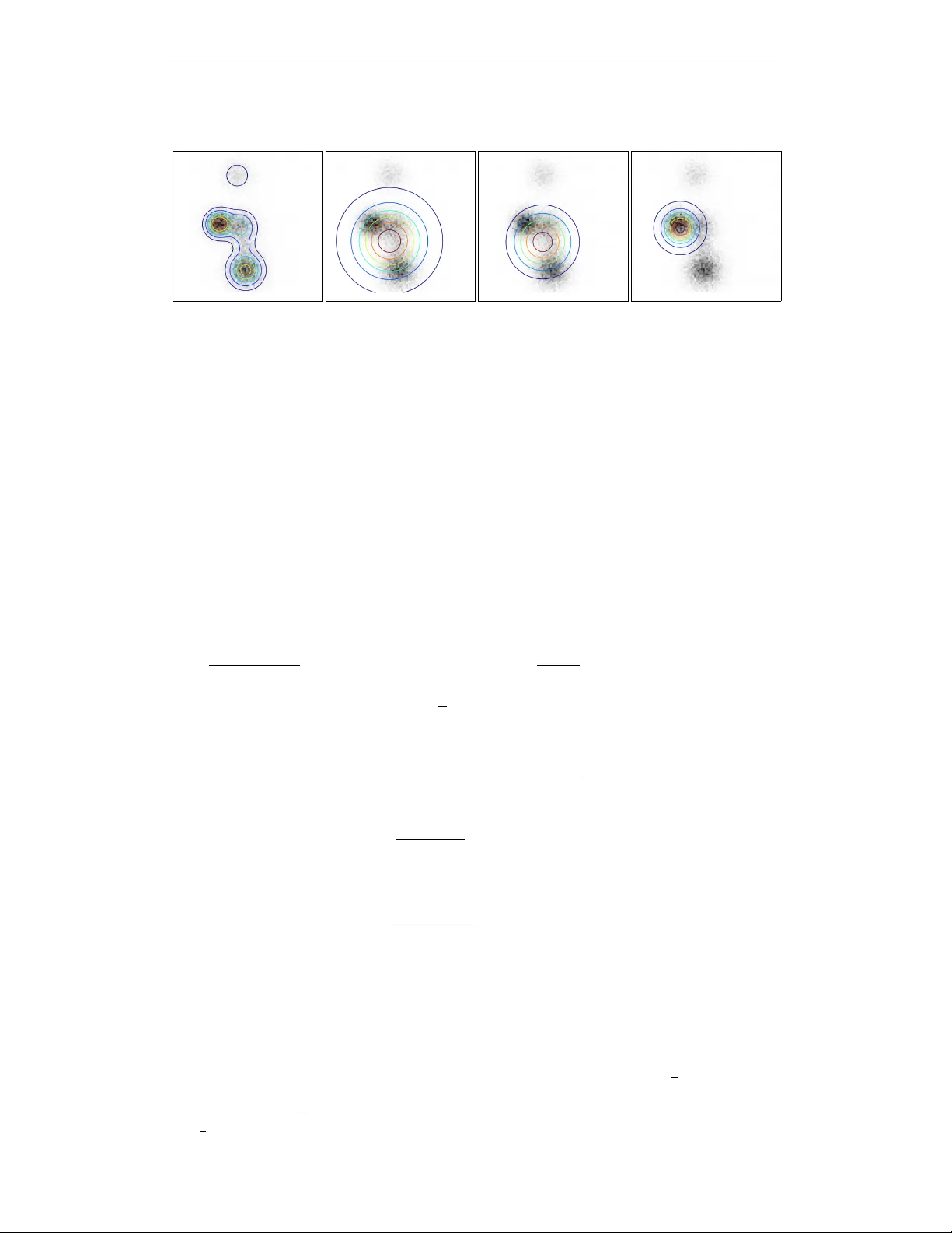
Modern applications and progress in deep learning research have created renewed interest for generative models of text and of images. However, even today it is unclear what objective functions one should use to train and evaluate these models. In thi…
Authors: Ferenc Huszar
Under revie w as a conference paper at ICLR 2016 H O W ( N O T ) T O T R A I N Y O U R G E N E R A T I V E M O D E L : S C H E D U L E D S A M P L I N G , L I K E L I H O O D , A D V E R S A RY ? Fer enc Husz ´ ar Balderton Capital LLP , London, UK ferenc.huszar@gmail.com A B S T R A C T Modern applications and progress in deep learning research hav e created rene wed interest for generativ e models of text and of images. Howe ver , even today it is unclear what objectiv e functions one should use to train and ev aluate these models. In this paper we present two contrib utions. Firstly , we present a critique of scheduled sampling, a state-of-the-art training method that contributed to the winning entry to the MSCOCO image captioning benchmark in 2015. Here we show that despite this impressive empirical per- formance, the objective function underlying scheduled sampling is improper and leads to an inconsistent learning algorithm. Secondly , we revisit the problems that scheduled sampling was meant to address, and present an alternati ve interpretation. W e argue that maximum likelihood is an inappropriate training objective when the end-goal is to generate natural-looking samples. W e go on to deriv e an ideal objectiv e function to use in this situation instead. W e introduce a generalisation of adv ersarial training, and sho w how such method can interpolate between maximum lik elihood training and our ideal train- ing objecti ve. T o our kno wledge this is the first theoretical analysis that e xplains why adversarial training tends to produce samples with higher percei ved quality . 1 I N T R O D U C T I O N Building sophisticated generati ve models that produce realistic-looking images or text is an impor- tant current frontier of unsupervised learning. The renewed interest in generative models can be attributed to two factors. Firstly , thanks to the acti ve in vestment in machine learning by internet companies, we now hav e sev eral products and practical use-cases for generati ve models: texture generation(Han et al., 2008), speech synthesis (Ou & Zhang, 2012), image caption generation (Lin et al., 2014; V in yals et al., 2014), machine translation (Sutske ver et al., 2014), con v ersation and dia- logue generation (V inyals & Le, 2015; Sordoni et al., 2015). Secondly , recent success in generativ e models, particularly those based on deep representation learning, ha ve raised hopes that our systems may one day reach the sophistication required in these practical use cases. While noticable progress has been made in generative modelling, in many applications we are still far from generating fully realistic samples. One of the key open questions is what objectiv e functions one should use to train and ev aluate generative models (Theis et al., 2015). The model likelihood is often considered the most principled training objective and most research in the past decades has focussed on maximum lieklihood(ML) and approximations thereof Hinton et al. (2006); Hyv ¨ arinen (2006); Kingma & W elling (2013). Recently we ha ve seen promising ne w training strategies such as those based on adversarial networks (Goodfellow et al., 2014; Denton et al., 2015) and kernel moment matching (Li et al., 2015; Dziugaite et al., 2015) which are not — at least on the surface — related to maximum likelihood. Most of this departure from ML was motiv ated by the fact that the exact likelihood is intractable in the most models. Howe ver , some authors have recently observ ed that ev en in models whose likelihood is tractable, ML training leads to undesired behaviour , and introduced ne w training procedures that deliberately differ from maximum lik elihood. Here we will focus on scheduled sampling (Bengio et al., 2015) which is an example of this. In this paper we attempt to clarify what objective functions might work well for the generativ e scenario and which ones should one av oid. In line with (Theis et al., 2015) and (Lacoste-Julien 1 Under revie w as a conference paper at ICLR 2016 et al., 2011), we belie ve that the objecti ve function used for training should reflect the task we want to ultimately use the model for . In the context of this paper , we focus on generativ e models that are created with the sole purpose of generating realistic-looking samples from. This narro wer definition extends to use-cases such as image captioning, texture generation, machine translation and dialogue systems, but excludes tasks such as unsupervised pre-training for supervised learning, semisupervised learning, data compression, denoising and many others. This paper is organised around the follo wing main contributions: scheduled sampling is improper: In the first half of this paper we focus on autore gressive models for sequence generation. These models are interesting for us mainly because exact max- imum likelihood training is tractable, ev en in relati vely complex models such as stacked LSTMs (Bengio et al., 2015; Sutske ver et al., 2014; Theis & Bethge, 2015). Howe ver , it has been observed that autoregressi ve generative models trained via ML hav e some un- desired behaviour when they are used to generate samples. W e re visit a recent attempt to remedy these problems: scheduled sampling. W e reexpress the scheduled sampling training objectiv e in terms of Kullback-Leibler diver gences, and show that it is in fact an improper training objectiv e. Therefore we recommend to use scheduled sampling with care. KL-diver gence as a model of perceptual loss: In the latter part of the paper we seek an alterna- tiv e solution to the problem scheduled sampling was meant to address. W e uncover a more fundamental problem that applies to all generative models: that the likelihood is not the right training objectiv e when the goal is to generate realistic samples. Maximum likelihood can be thought of as minimising the Kullback-Leibler diver gence K L [ P k Q ] between the real data distribution P and the probabilistic model Q . W e present a model that suggests generativ e models should instead be trained to minimise K L [ Q k P ] , the K ullback-Leibler div ergence in the opposite direction. The differences between minimising K L [ P k Q ] and K L [ Q k P ] are well understood, and e xplain the observed undesirable behaviour in autore- gressiv e sequence models. generalised adversarial training: Unfortunately , K L [ Q k P ] is e ven harder to optimise than the likelihood, so it is unlikely to yield a viable training procedure. Instead, we suggest to min- imise an information quantity which we call generalised Jensen-Shannon div ergence. W e show that this diver gence can effecti vely interpolate between the behaviour of K L [ P k Q ] and K L [ P k Q ] , thereby containing both maximum likelihood, and our ideal perceptual objectiv e function as a special case. W e also show that generalisations of the adversarial training procedure proposed in (Goodfellow et al., 2014) can be employed to approximately minimise this div ergence function. Our analysis also provides a new theoretical explanation for the success of adversarial training in producing qualitati vely superior samples. 2 A U T O R E G R E S S I V E M O D E L S F O R S E Q U E N C E G E N E R A T I O N In this section we will focus on a particularly useful class of probabilistic models, which we call autoregressi ve generative models (see e. g. Theis et al., 2012; Larochelle & Murray, 2011; Bengio et al., 2015). An autoregressi ve probabilistic model explicitly defines the joint distribution ov er a sequence of symbols x 1: N recursiv ely as follows: Q 1: N ( x 1: N ) = N Y n =1 Q n ( x n | x 1: n − 1 ; θ ) . (1) W e note that technically the above equation holds for all joint distributions Q 1: N , here we fur- ther assume that each of the component distributions Q n ( x n | x 1: n − 1 ; θ ) . are tractable and easy to compute. Autoregressi ve models are considered relatively easy to train, as the model likelihood is typically tractable. This allo ws us to train e ven complicated deep models such as stacked LSTMs in the coherent and well understood frame work of maximum likelihood estimation (Theis et al., 2012; 2015). 2 Under revie w as a conference paper at ICLR 2016 3 T H E S Y M P T O M S Despite the elegance of a closed-form maximum likelihood training, Bengio et al. (2015) have ob- served out that maximum likelihood training leads to undesirable beha viour when the models are used to generate samples from. In this section we revie w these symptoms , and throughout this paper we will explore dif ferent strategies aimed at explaining and T ypically , when training an AR model, one minimises the log predictiv e likelihood of the n th symbol in each training sentence conditioned on all previous symbols in the sequence that we collecti vely call the prefix. This can be thought of as a special case of maximum likelihood learning, as the joint likelihood over all symbols in a sequence factorises into these conditionals via the chain rule of probabilities. When using the trained model to generate sample sequences, we generate each new sequence symbol-by-symbol in a recursive fashion: Assuming we already generated a prefix of n sybols, we feed that prefix into the conditional model, and ask it to output the predictiv e distribution for the n + 1 st character . The n + 1 st character is then sampled from this distrib ution and added to the prefix. Crucially , at training time the RNN only sees prefixes from real training sequences. Ho wever , at generation time, it can generate a prefix that is ne ver seen in the training data. Once an unlikely prefix is generated, the model typically has a hard time recovering from the mistake, and will start outputting a seemingly random string of symbols ending up with a sample that has poor perceptual quality and is very unlikely under the true sequence distrib ution P . 4 S Y M P T O M A T I C T R E A T M E N T : S C H E D U L E D S A M P L I N G In (Bengio et al., 2015), the authors stipulate that the cause of the observed poor behaviour is the disconnect between ho w the model is trained (it’ s alw ays fed prefixes from real data) and ho w it’ s used (it’ s always fed synthetic prefixes generated by the model itself). T o address this, the authors propose an alternative training strategy called scheduled sampling (SS). In scheduled sampling, the network is sometimes given its own synthetic data as prefix instead of a real prefix at training time. This, the authors argue, simulates the environment in which the model is used when generating samples from it. More specifically , we turn each training sequence into modified training sequence in a recursiv e fashion using the follo wing procedure: • for the n th symbol we draw from a Bernoulli distribution with parameter to decide whether we keep the original symbol or use one generated by the model • if we decided to replace the symbol, we use the current model RNN to output the predictiv e distribution of the next symbol giv en the current prefix, and sample from this predictiv e distribution • we add to the training loss the log predictive probability of the real n th symbol, gi ven the prefix (the prefix at this point may already contain generated characters) • depending on the coinflip above, the original or simulated character is added to the prefix and we continue with the recursion The method is called scheduled sampling to describe the way the hyperparameter is annealed during training from an initial value of = 1 down to = 0 . Here, we would like to understand the limiting behaviour of this training procedure, whether and why it is an appropriate way to address the shortcomings of maximum likelihood training. 4 . 1 S C H E D U L E D S A M P L I N G F O R M U L A T E D A S K L D I V E R G E N C E M I N I M I S AT I O N T o keep notation simple, let us consider the case of learning sequences of length 2, that is pairs of random symbols x 1 and x 2 . Our aim is to formulate a closed form training objective that corresponds to scheduled sampling. 3 Under revie w as a conference paper at ICLR 2016 If x 1 is kept original - rather than replaced by a sample - the scheduled sampling objectiv e in fact remains the same as maximum likelihood. W e can understand maximum likelihood as minimising the following KL di ver gence 1 between the true data distribution P and our approximation Q : D M L [ P k Q ] = K L [ P k Q ] (2) = K L [ P x 1 k Q x 1 ] + E z ∼ P x 1 K L [ P x 2 | x 1 = z k Q x 2 | x 1 = z ] (3) Here, P x 1 and Q x 1 denote marginal distributions of the first symbol x 1 under P and Q respec- tiv ely , while Q x 2 | x 1 = z and P x 2 | x 1 = z denote the conditional distributions of the second symbol x 2 conditioned on the value of the first symbol x 1 being z . The other case we need to consider is when x 1 is replaced by a sample from the model, in this case Q x 1 . The training objectiv e can now be expressed as the follo wing div ergence: D alter native [ P k Q ] = K L [ P x 1 k Q x 1 ] + E y ∼ P x 1 E z ∼ Q x 1 K L [ P x 2 | x 1 = y k Q x 2 | x 1 = z ] (4) = K L [ P x 1 k Q x 1 ] + E z ∼ Q x 1 K L [ P x 2 k Q x 2 | x 1 = z ] (5) Notice how in the second term the KL diver gence is now measured from P x 2 rather than the condi- tional, this is because the real value of the first symbol is ne ver shown to the model, when it is asked to predict the second symbol x 2 . In scheduled sampling, we choose randomly between the abov e two cases, so the full SS objecti ve can be described as a con vex combination of D M L and D alter native abov e: D S S [ P k Q ] = K L [ P x 1 k Q x 1 ]+ E z ∼ P x 1 K L [ P x 2 | x 1 = z k Q x 2 | x 1 = z ]+(1 − ) E z ∼ Q x 1 K L [ P x 2 k Q x 2 | x 1 = z ] (6) It is worth noting at this point that this di vergence is an idealised form of the scheduled sampling. In the actual algorithm, expectations o ver Q x 1 and B er noull i ( ) would be implemented by sampling 2 . This div ergence describes the method’ s limiting behaviour in the limit of infinite training data. By rearranging terms we can further express the SS objecti ve as the follo wing KL diver gence: D S S [ P k Q ] = K L [ P x 1 k Q x 1 ] + E z ∼ P x 1 K L P x 1 | x 1 = z + Q x 1 ( z ) Q x 1 ( z ) P x 2 Q x 2 | x 1 = z + C P, (7) = K L P x 1 P x 1 | x 1 + (1 − ) Q x 1 P x 2 P x 1 Q x 1 ,x 2 + C P, (8) A very natural requirement for an y di ver gence function used to assess goodness of fit in probabilistic models is that it is minimised when Q = P . In statistics, this property is referred to as strictly proper scoring rule estimation (Gneiting & Raftery, 2007). W orking with strictly proper di vergences guarantees consistency , i. e. that the training procedure can ultimately recov er the true P , assuming the model class is flexible enough and enough training data is provided. What the above analysis shows us is that scheduled sampling is not a consistent estimation strategy . As → 0 , the di ver gence is globally minimised at the factorised distribution Q = P x 1 P x 2 , rather than at the correct joint distribution P . The model is still inconsistent when intermediate values 0 < < 1 are used, in this case the di vergence has a global optimum that is somewhere between the true joint P and the factorised distrib ution P x 1 P x 2 . Based on this analysis we suggest that scheduled sampling works by pushling models towards a trivial solution of memorising distrib ution of symbols conditioned on their position in the sequence, 1 more precisely , maximum likelihood minimises the cross-entropy K L [ P k Q ] + H [ P ] , where H [ P ] is the differential entrop y of training data. 2 The authors also propose taking argmax of each distrib ution instead of sampling, this case is harder to analyse but we think our general observ ations still hold. 4 Under revie w as a conference paper at ICLR 2016 rather than on the prefix of preceding symbols. In recurrent neural network (RNN) terminology , this would means that the optimal architecture under SS uses its hidden states merely to implement a simple counter , and learns to pay no attention whatsoev er to the content of the sequence prefix. While this may indeed lead to models that are more likely to recov er from mistakes, we believ e it fails to address the limitations of maximum likelihood the authors initially set out to solv e. How could an inconsistent training procedure still achiev e state-of-the-art performance in the image captioning challenge? There are multiple possible explanations to this. W e speculate that the optimi- sation was not run until full con vergence, and perhaps an improv ement over the maximum lik elihood solution was found as a coincidence due to the the interplay between early stopping, random restarts, the specific structure of the model class and the annealing schedule for . 5 T H E D I A G N O S I S After discussing scheduled sampling, a method proposed to remedy the symptoms explained in section 3, we now seek a better explanation of why those symptoms exist in the first place. W e will now lea ve the autore gressive model class, and consider probabilistic generati ve models in their full generality . The symptoms outlined in Section 3 can be attributed to a mismatch between the loss function used for training (lik elihood) and the loss used for ev aluating the model (the perceptual quality of samples produced by the model). T o fix this problem we need a training objecti ve that more closely matches the perceptual metric used for ev aluation, and ideally one that allo ws for a consistent statistical estimation framew ork. 5 . 0 . 1 A M O D E L O F N O - R E F E R E N C E P E R C E P T UA L Q UA L I T Y A S S E S S M E N T When researchers e valuate their generati ve models for perceptual quality , the y draw samples from it, then - for lack of a better word - e yeball the samples. In visual information processing this is often referred to as no-reference perceptual quality assessment (see e. g. W ang et al., 2002). When using the model in an application like caption generation, we typically draw a sample from a conditional model y | x ∼ Q y | x , where mathbf x represents the context of the query , and present it to a human observer . W e would like each sample to pass a T uring test. W e want the human observer to feel like y is a plausible naturally occurring response, within the context of the query x . In this section, we will propose that the KL di vergence K L [ Q k P ] can be used as an idealised objectiv e function to describe the no-reference perceptual quality assessment scenario. First of all, we make the assumption that the perceiv ed quality of each sample is related to the surprisal − log Q human ( x ) under the human observers’ subjectiv e prior of stimuli Q human ( x ) CITE. W e further assume that the human observer has learnt an accurate model of the natural distrib ution of stimuli, thus, Q human ( x ) = P ( x ) . These two assumptions suggest that in order to optimise our chances in the T uring test scenario, we need to minimise the follo wing cross-entropy or perplexity term: − E x ∼ Q log P ( x ) (9) Note that this perplexity is the exact opposite a verage ne gative log likelihood − E x ∼ P log Q ( x ) , wit h the role of P and Q changed. Howe ver , the objecti ve in Eqn. 9 w ould be maximised by a model Q that deterministically picks the most likely stimulus. T o enforce div ersity one can simultaneously try to maximise the entropy of Q . This leav es us with the following KL di vergence to optimise: K L [ Q k P ] = − E x ∼ Q log P ( x ) + E x ∼ Q log Q ( x ) (10) It is kno wn that K L [ Q k P ] is minimised when P = Q , therefore minimising it would correspond to a consistent estimation strate gy . Howe ver , it is only well-defined when P is positi ve and bounded in the full support of Q , which is not the case when P is an empirical distribution of samples and Q is a smooth probabilistic model. For this reason, K L [ Q k P ] is not viable as a practical training objecti ve 5 Under revie w as a conference paper at ICLR 2016 in statistical esimation. Still, we can use it as our idealised perceptual quality metric to motiv ate our choice of practical objectiv e functions. 5 . 0 . 2 H O W D O E S T H I S E X P L A I N T H E S Y M P T O M S ? The differences in beha viour between K L [ Q k P ] and K L [ P k Q ] are well understood and exploited for e xample in the conte xt of approximate Bayesian inference (Lacoste-Julien et al., 2011; MacKay, 2003; Minka, 2001). The differences are most visible when model underspecification is present: imagine trying to model a multimodal P with a simpler , unimodal model Q . Minimising K L [ P k Q ] corresponds to moment matching and has a tendency to find models Q that co ver all the modes of P , at the cost of placing probability mass where P has none. Minimising K L [ Q k P ] in this case leads to a mode-seeking beha viour: the optimal Q will typically concentrate around the largest mode of P , at the cost of completely ignoring smaller modes. These differences are illustrated visually in Figure 1, panels B and D. In the context of generative models this means that minimising K L [ P k Q ] often leads to models that over generalise, and sometimes produce samples that are very unlikely under P . This would explain why recurrent neural networks trained via maximum likelihood also hav e a tendency to produce completely unseen sequences. Minimising K L [ P k Q ] will aim to create a model that can generate all the behaviour that is observed in real data, at the cost of introducing beha viours that are ne ver seen. By contrast, if we train a generativ e model by minimising K L [ Q k P ] , the model will very conservati vely try to avoid any behaviour that is unlikely under P . This comes at the cost of ignoring modes of P completely , unless those additional modes can be modelled without introducing probability mass in regions where P has none. Once again, both K L [ P k Q ] and K L [ Q k P ] define consistent estimation strategies. They differ in the kind of errors they make under se vere model misspecification particularly in high dimensions. 6 G E N E R A L I S E D A DV E R S A R I A L T R A I N I N G W e theorised that K L [ Q k P ] may be a more meaningful training objecti ve if our aim w as to impro ve the perceptual quality of generativ e models, but it is impractical as an objecti ve function. Here we show that a generalised version of adversarial training (Goodfellow et al., 2014) can be used to approximate training based on K L [ Q k P ] . Adversarial training can be described as minimising an approximation to the Jensen-Shannon di vergence between P and Q (Goodfellow et al., 2014; Theis et al., 2015). The JS div ergence between P and Q is defined by the following formula: J S D [ P k Q ] = J S D [ P k Q ] = 1 2 K L P P + Q 2 + 1 2 K L Q P + Q 2 (11) Unlike KL di vergence, the JS div ergence is symmetric in its arguments, and can be understood as being somewhere between K L [ Q k P ] and K L [ P k Q ] in terms of its behaviour . One can therefore hope that JSD would behav e a bit more like K L [ Q k P ] and therefore ultimately tend to produce more realistic samples. Indeed, the behaviour of JSD minimisation under model misspecification is more similar to K L [ Q k P ] than K L [ P k Q ] as illustrated in Figure 1. Empirically , methods built on adversarial training do tend to produce appealing samples (Goodfellow et al., 2014; Denton et al., 2015). Howe ver , we can ev en formally show that JS div ergence is indeed an interpolation between the two KL div ergences in the follo wing sense. Let us consider a more general definition of Jensen-Shannon div ergence, parametrised by a non-tri vial probability 0 < π < 1 : J S π [ P k Q ] = π · K L [ P k πP + (1 − π ) Q ] + (1 − π ) K L [ Q k πP + (1 − π ) Q ] . (12) For any gi ven value of π this generalised Jensen-Shannon diver gence is not symmetric in its argu- ments P and Q anymore, instead the follo wing weaker notion of symmetry holds: J S π [ P k Q ] = J S 1 − π [ Q k P ] (13) 6 Under revie w as a conference paper at ICLR 2016 A: P B: arg min Q J S 0 . 1 [ P k Q ] C: arg min Q J S 0 . 5 [ P k Q ] D: arg min Q J S 0 . 99 [ P k Q ] Figure 1: Illustrating the behaviour of the generalised JS di vergence under model underspecification for a range of values of π . Data is drawn from a multi variate Gaussian distrib ution P (A) and we aim approximate it by a single isotropic Gaussian (B-D) . Contours show level sets the approximating distribution, overlaid on top of the 2D histogram of observed data. For π = 0 . 1 , JS div ergence minimisation beha ves like maximum lik elihood (B) , resulting in the characteristic moment matching behaviour . For π = 0 . 99 (D) , the behaviour becomes more akin to the mode-seeking beha viour of minimising K L [ Q k P ] . For the intermediate value of π = 0 . 5 (C) we recover the standard JS div ergence approximated by adversarial training. T o produce this illustraiton we used software made av ailable by Theis et al. (2015). It is easy to sho w that J S π div ergence conv erges to 0 in the limit of both π → 0 and π → 1 . Cru- cially , it can be shown that the gradients with respect to π at these two extremes recover K L [ Q k P ] and K L [ P k Q ] , respectiv ely . A proof of this property can be obtained by considering the T aylor- expansion K L [ Q k Q + a ] ≈ a T H a , where H is the positiv e definite Hessian and substituting a = π ( P − Q ) as follows: lim π → 0 J S D [ P k Q ; π ] π = lim π → 0 K L [ P k πP + (1 − π ) Q ] + 1 − π ) π K L [ Q k πP + (1 − π ) Q ] (14) = K L [ P k Q ] + lim π → 0 1 π π 2 ( P − Q ) T H ( P − Q ) (15) = K L [ P k Q ] (16) Therefore, we can say that for infinitisemally small v alues of π , J S π is approximately proportional to K L [ P k Q ] : J S π [ P k Q ] π ≈ K L [ P k Q ] . (17) And by symmetry in Eqn. 13 we also hav e that for small values of π J S 1 − π [ P k Q ] 1 − π ≈ K L [ Q k P ] (18) This limiting behaviour also implies that for small values of π , J S π has the same optima as K L [ P k Q ] . For values of π close to 1 , J S π has the same optima as K L [ Q k P ] . Thus, by min- imising J S π div ergence for a range of π ∈ (0 , 1) allows us to interpolate between the behaviour of K L [ P k Q ] and K L [ Q k P ] . W e note that J S π can also be approximated via adversarial training as described in (Goodfello w et al., 2014). The practical meaning of the parameter π is the ratio of labelled samples the adv ersarial disctiminator network receiv es from Q and P in the training procedure. π = 1 2 implies that the adversarial network is faced with a balanced classification problem as it is the case in the original algorithm, for π < 1 2 samples from the real distribution P are overrepresented. Similarly , when π > 1 2 , the classification problem is biased to wards Q . Thus, the generality of generati ve adv ersarial 7 Under revie w as a conference paper at ICLR 2016 networks can be greatly improved by incorporating a minor change to the procedure. W e note that this change may ha ve adverse ef fects on the con vergence properties of the algorithm, which we hav e not in vestigated. 7 C O N C L U S I O N S In this paper our goal was to understand which objecti ve functions work and which ones don’t in the context of generative models. Here we were only interested in models that are created for the purpose of dra wing samples from, and we e xcluded other use-cases such as semi-supervised feature learning. Our findings and recommendations can be summarised as follows: 1. Maximum likelihood should not be used as the training objecti ve if the end goal is to dra w realistic samples from the model. Models trained via maximum likelhiood ha ve a tendency to ov ergeneralise and generate unplausible samples. 2. Scheduled sampling, designed to o vercome the shortcomings of maximum likelihood, fails to address the fundamental problems, and we sho wed it is an inconsistent training strate gy . 3. W e theorise that K L [ Q k P ] could be used as an idealised objecti ve function to describe the no-reference perceptual quality assessment scenario, but it is impractical to use in practice. 4. W e propose the generalised Jensen-Shannon di vergence as a promising, more tractable objectiv e function that can ef fectively interpolate between maximum likelihood and K L [ Q k P ] -minimisation. 5. Our analysis suggests that adversarial training strategies are a the best choice for gener- ativ e modelling, and we propose a more flexible algorithm based on our generalised JS div ergence. While our analysis highlighted the merits of adversarial training, it should be noted that the method is still very new , and has serious practical limitations. Firstly , the generativ e adversarial network algorithm is based on sampling from the approximate model Q , which is highly inefficient in high dimensional spaces. This limits the applicability of these methods to low-dimensional problems, and increases sensiti vity to hyperparameters. Secondly , it is unclear how to employ adversarial traning on discrete probabilistic models, where the sampling process cannot be described as a dif ferentiable operation. T o make adversarial training practically viable these limitations need to be addressed in future work. A C K N OW L E D G M E N T S I would like to thank Lucas Theis and Hugo Larochelle for useful discussions. I would like to thank authors Theis, van den Oord, and Bethge (2015) for kindly providing the source code for creating illustrations in Figure 1. R E F E R E N C E S Bengio, Samy , V inyals, Oriol, Jaitly , Na vdeep, and Shazeer, Noam M. Scheduled sampling for se- quence prediction with recurrent neural networks. In Advances in Neural Information Pr ocessing Systems, NIPS , 2015. URL . Denton, Emily , Chintala, Soumith, Szlam, Arthur, and Fer gus, Rob. Deep generative image models using a laplacian pyramid of adversarial netw orks. arXiv pr eprint arXiv:1506.05751 , 2015. Dziugaite, Gintare Karolina, Ro y , Daniel M, and Ghahramani, Zoubin. T raining generativ e neural networks via maximum mean discrepancy optimization. arXiv pr eprint arXiv:1505.03906 , 2015. Gneiting, T ilmann and Raftery , Adrian E. Strictly proper scoring rules, prediction, and estimation. Journal of the American Statistical Association , 102(477):359–378, 2007. 8 Under revie w as a conference paper at ICLR 2016 Goodfellow , Ian, Pouget-Abadie, Jean, Mirza, Mehdi, Xu, Bing, W arde-Farley , David, Ozair, Sher- jil, Courville, Aaron, and Bengio, Y oshua. Generative adv ersarial nets. In Advances in Neural Information Pr ocessing Systems , pp. 2672–2680, 2014. Han, Charles, Risser , Eric, Ramamoorthi, Ravi, and Grinspun, Eitan. Multiscale texture synthesis. A CM T ransactions on Graphics (Pr oceedings of SIGGRAPH 2008) , 27(3):51:1–51:8, 2008. Hinton, Geof frey E, Osindero, Simon, and T eh, Y ee-Whye. A fast learning algorithm for deep belief nets. Neural computation , 18(7):1527–1554, 2006. Hyv ¨ arinen, Aapo. Consistency of pseudolik elihood estimation of fully visible boltzmann machines. Neural Computation , 18(10):2283–2292, 2006. Kingma, Diederik P and W elling, Max. Auto-encoding v ariational bayes. arXiv pr eprint arXiv:1312.6114 , 2013. Lacoste-Julien, Simon, Husz ´ ar , Ferenc, and Ghahramani, Zoubin. Approximate inference for the loss-calibrated bayesian. In International Conference on Artificial Intellig ence and Statistics , pp. 416–424, 2011. Larochelle, Hugo and Murray , Iain. The neural autoregressi ve distribution estimator . In Interna- tional Confer ence on Artificial Intelligence and Statistics , pp. 29–37, 2011. Li, Y ujia, Swersky , K evin, and Zemel, Richard. Generativ e moment matching networks. arXiv pr eprint arXiv:1502.02761 , 2015. Lin, Tsung-Y i, Maire, Michael, Belongie, Serge, Hays, James, Perona, Pietro, Ramanan, Dev a, Doll ´ ar , Piotr , and Zitnick, C La wrence. Microsoft coco: Common objects in context. In Computer V ision–ECCV 2014 , pp. 740–755. Springer , 2014. MacKay , David JC. Information theory , inference and learning algorithms . Cambridge univ ersity press, 2003. Minka, Thomas P . A family of algorithms for appr oximate Bayesian infer ence . PhD thesis, Mas- sachusetts Institute of T echnology , 2001. Ou, Zhijian and Zhang, Y ang. Probabilistic acoustic tube: a probabilistic generati ve model of speech for speech analysis/synthesis. In International Conference on Artificial Intelligence and Statistics , pp. 841–849, 2012. Sordoni, Alessandro, Galley , Michel, Auli, Michael, Brockett, Chris, Ji, Y angfeng, Mitchell, Mar- garet, Nie, Jian-Y un, Gao, Jianfeng, and Dolan, Bill. A neural network approach to context- sensitiv e generation of con versational responses. arXiv pr eprint arXiv:1506.06714 , 2015. Sutske ver , Ilya, V inyals, Oriol, and Le, Quoc VV . Sequence to sequence learning with neural net- works. In Advances in neural information pr ocessing systems , pp. 3104–3112, 2014. Theis, Lucas and Bethge, Matthias. Generati ve image modeling using spatial lstms. arXiv preprint arXiv:1506.03478 , 2015. Theis, Lucas, Hosseini, Reshad, Bethge, Matthias, and Hsiao, Chuhsing Kate. Mixtures of condi- tional gaussian scale mixtures applied to multiscale image representations. PloS one , 7(7):e39857, 2012. Theis, Lucas, van den Oord, Aaron, and Bethge, Matthias. A note on the e valuation of generati ve models. arXiv:1511.01844, Nov 2015. URL . V inyals, Oriol and Le, Quoc. A neural conv ersational model. arXiv preprint , 2015. V inyals, Oriol, T oshev , Alexander , Bengio, Samy , and Erhan, Dumitru. Sho w and tell: A neural image caption generator . arXiv preprint , 2014. W ang, Zhou, Sheikh, Hamid R, and Bovik, Alan C. No-reference perceptual quality assessment of jpeg compressed images. In Ima ge Pr ocessing. 2002. Pr oceedings. 2002 International Confer ence on , volume 1, pp. I–477. IEEE, 2002. 9
Original Paper
Loading high-quality paper...
Comments & Academic Discussion
Loading comments...
Leave a Comment