Fast Algorithms for Convolutional Neural Networks

Deep convolutional neural networks take GPU days of compute time to train on large data sets. Pedestrian detection for self driving cars requires very low latency. Image recognition for mobile phones is constrained by limited processing resources. The success of convolutional neural networks in these situations is limited by how fast we can compute them. Conventional FFT based convolution is fast for large filters, but state of the art convolutional neural networks use small, 3x3 filters. We introduce a new class of fast algorithms for convolutional neural networks using Winograd’s minimal filtering algorithms. The algorithms compute minimal complexity convolution over small tiles, which makes them fast with small filters and small batch sizes. We benchmark a GPU implementation of our algorithm with the VGG network and show state of the art throughput at batch sizes from 1 to 64.

💡 Research Summary

The paper addresses a critical bottleneck in modern deep learning: the high computational cost of convolutional neural networks (CNNs) when using small 3×3 kernels and small batch sizes, which are common in real‑time applications such as autonomous‑vehicle perception and mobile image recognition. While FFT‑based convolution can reduce arithmetic complexity for large filters, it is inefficient for the 3×3 kernels that dominate state‑of‑the‑art architectures (e.g., VGG, ResNet).

The authors propose a new class of fast convolution algorithms based on Winograd’s minimal filtering theory. For a 1‑D FIR filter of length r producing m outputs, the minimal number of multiplications is µ(F(m,r)) = m + r − 1. By nesting these 1‑D algorithms, a 2‑D minimal algorithm F(m×n, r×s) requires only (m + r − 1)(n + s − 1) multiplications, compared with the naïve m·n·r·s multiplications of direct convolution. This reduction can be up to a factor of four for typical tile sizes.

The paper details three concrete instantiations:
* F(2×2, 3×3) – computes a 2×2 output tile from a 4×4 input tile using 16 multiplications (vs. 36 for direct). The data, filter, and inverse transforms are expressed as small constant matrices Bᵀ, G, Aᵀ, and the core computation becomes an element‑wise product of transformed matrices followed by an inverse transform.
* F(3×3, 2×2) – used for back‑propagation where gradients with respect to weights require a convolution of the input with the error map. By tiling the large error map into 2×2 output blocks, the same Winograd machinery can be reused.
* F(4×4, 3×3) – demonstrates the theoretical limit of the approach (36 multiplications vs. 144 for direct), but also shows that the transform overhead (additions, constant multiplications) grows quadratically with tile size, eventually outweighing the multiplication savings and degrading numerical stability.

Algorithm 1 in the paper outlines the full GPU implementation: each input channel is tiled, transformed (data transform Bᵀ), each filter is transformed (filter transform G), the transformed tensors are multiplied using dense GEMM (highly optimized on GPUs), and finally the inverse transform Aᵀ produces the output tiles. Crucially, the transforms are performed once per channel and once per filter, then summed across channels before the inverse transform, amortizing the inverse‑transform cost.

The authors compare their Winograd approach with FFT‑based convolution. FFT requires complex‑valued transforms and, even with Hermitian symmetry optimizations, needs at least 2 real multiplications per input element (or 3 with fast complex multiplication tricks). In contrast, Winograd’s multiplication stage always uses exactly one real multiplication per input element. Moreover, FFT’s transform overhead and memory footprint increase with tile size, making it less competitive for the small tiles that give the best speed‑up in practice.

Complexity analysis shows that the total multiplication count for a layer is
M = N·⌈H/m⌉·⌈W/n⌉·C·K·(m + R − 1)(n + S − 1).
When m = n = 1, this collapses to direct convolution, confirming that Winograd is a strict generalization that reduces arithmetic when m,n > 1. The authors note that further reductions could be achieved with Strassen‑style recursion, but the benefit (≈8/7) is modest compared with the 2–4× gains already obtained.

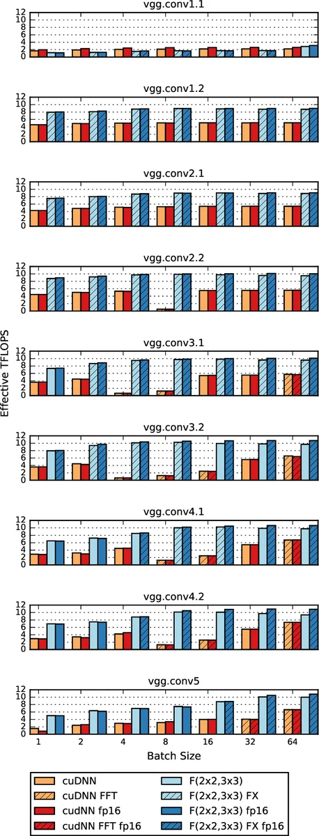
Experimental evaluation is performed on an NVIDIA Maxwell GPU using the VGG‑16 network. Throughput is measured for batch sizes from 1 to 64. The Winograd implementation achieves 2.2×–4.3× higher images‑per‑second than cuDNN’s FFT‑based convolution, while using at most 16 MB of auxiliary workspace. The performance advantage is most pronounced at the smallest batch sizes, where traditional libraries suffer from low GPU occupancy.

In conclusion, the paper demonstrates that Winograd minimal filtering provides a practical, mathematically optimal way to accelerate CNNs with small kernels and small batches. By mapping the theory to dense GEMM operations, the authors exploit the strengths of modern GPUs, achieving state‑of‑the‑art throughput with modest memory requirements. The work opens the door for real‑time deep‑learning inference on resource‑constrained platforms such as autonomous vehicles and mobile devices.