Sparse Variational Bayesian Approximations for Nonlinear Inverse Problems: applications in nonlinear elastography

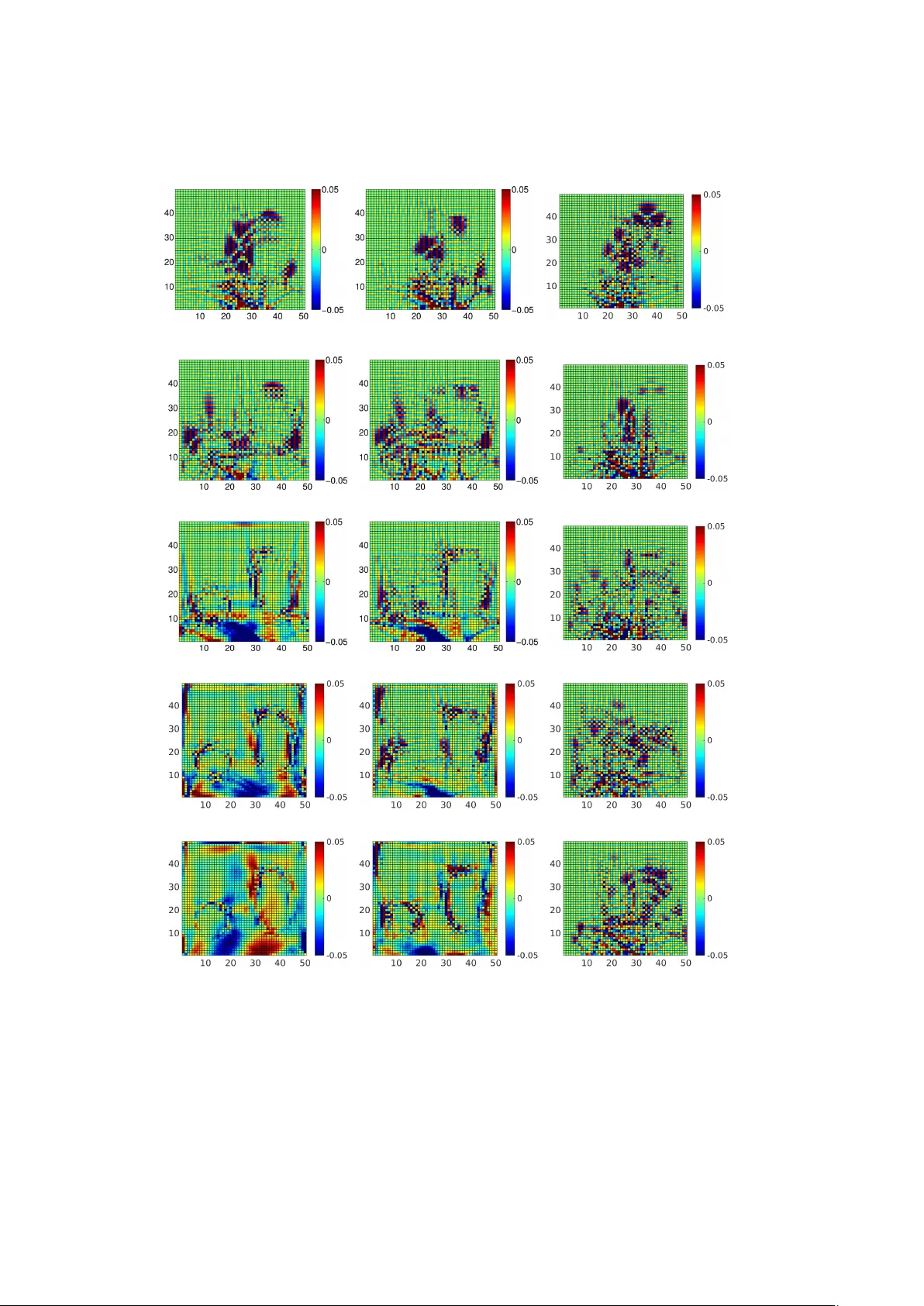
Sparse V ariational Bay esian Appro ximations f or Nonlinear In verse Prob lems: applications in nonlinear elastogr aphy Isabell M. F ranck a , P .S. K outsourelakis a, ∗ a Professur f ¨ ur K ontinuumsmechanik, T echnische Universit ¨ at M ¨ unchen, Boltzmannstrasse 15, 85747 Garching (b . M ¨ unchen), Germany Abstract This paper presents an efficient Ba yesian frame work for solving nonlinear , high-dimensional model calibration problems . It is based on a V ariational Ba yesian formulation that aims at ap- pro ximating the exact posterior by means of solving an optimization problem ov er an appro- priately selected f amily of distributions. The goal is two-f old. Firstly , to find lower-dimensional representations of the unknown parameter vector that capture as much as possible of the associated poster ior density , and secondly to enable the computation of the approximate posterior density with as fe w forward calls as possible. W e discuss how these objectives can be achiev ed b y using a fully Bay esian argumentation and emplo ying the marginal like- lihood or evidence as the ultimate model v alidation metric for any proposed dimensionality reduction. We demonstrate the perf or mance of the proposed methodology f or problems in nonlinear elastograph y where the identification of the mechanical proper ties of biological materials can inf or m non-inv asive , medical diagnosis. An Impor tance Sampling scheme is finally emplo yed in order to v alidate the results and assess the efficacy of the appro ximations provided. K eywords: Uncer tainty Quantification, V ariational Ba yesian, Inv erse Problem, Dimensionality reduction, Elastograph y, Dictionar y Learning Cop yr ight c  2015 I. M. Fr anck and P .S. K outsourelakis. This manuscript v ersion is made av ailable under the CC-BY -NC-ND 4.0 license http://creativecommons.org/licenses/ by- nc- nd/4.0/ 1. Introduction The e xtensiv e use of large-scale computational models poses sev eral challenges in model calibration as the accuracy of the predictions pro vided depends strongly on assigning proper values to the various model parameters . In mechanics of materials, accurate me- chanical proper ty identification can guide damage detection and an inf ormed assessment of the system’ s reliability [1]. Identifying proper ty-cross correlations can lead to the design of ∗ Corresponding Author . T el: +49-89-289-16690 Email addresses: franck@tum.de (Isabell M. F ranck), p.s.koutsourelakis@tum.de (P .S. K outsourelakis) URL: http://www.contmech.mw.tum.de (P .S. K outsourelakis) Preprint submitted to Computer Methods in Applied Mechanics and Engineering October 4, 2018 multi-functional materials [2]. P er meability estimation for soil transport processes can assist in detection of contaminants, oil e xploration [3]. Deterministic optimization techniques which ha ve been dev eloped to address these prob- lems [4], lead to point estimates f or the unknowns without rigorously considering the statisti- cal nature of the problem and without providing quantification of the uncer tainty in the in verse solution. Statistical approaches based on the Ba yesian paradigm [5] on the other hand, aim at computing a (posterior) probability distr ibution on the parameters of interest. Ba yesian for- mulations offer sev eral advantages as they provide a unified framework for dealing with the uncer tainty introduced by the incomplete and noisy measurements. Significant successes hav e been noted in applications such as geological tomograph y [6] , medical tomograph y [7], petroleum engineer ing [8] , as well as a host of other ph ysical, biological, or social sys- tems [9, 10]. Representations of the parametric fields in e xisting deter ministic and Bay esian approaches (ar tificially) impose a minimum length scale of variability usually deter mined by the discretization size of the governing PDEs [11]. As a result they give rise to a ver y large vector of unknowns. Inf erence in high-dimensional spaces using standard Markov Chain Monte Car lo (MCMC) schemes is generally impractical as it requires an exuber ant number of calls to the f orward simulator in order to achie ve convergence . Advanced schemes such as those employing Sequential Monte Car lo samplers [12, 13], adaptive MCMC [14], accel- erated MCMC methods [15] or spectral methods [16] can alleviate some of these difficulties par ticularly when the poster ior is multi-modal but still pose significant challenges in terms of the computational cost [17]. This work is par ticularly concer ned with the identification of the mechanical properties of biological materials, in the context non-inv asive medical diagnosis. While in cer tain cases mechanical proper ties can also be measured directly by e xcising multiple tissue samples, non-inv asive procedures off er obvious advantages in ter ms of ease, cost and reducing r isk of complications to the patient. Rather than x-r ay techniques which capture v ar iations in den- sity , the identification of stiffness or mechanical proper ties in general, can potentially lead to earlier and more accurate diagnosis [18, 19], provide valuab le insights that diff erentiate be- tween modalities of the same pathology [20] and monitor the progress of treatments. In this paper we do not propose new imaging techniques b ut rather aim at de veloping rigorous sta- tistical models and efficient computational tools that can mak e use of the data/observables (i.e. noisy displacements of def or med tissue) from e xisting imaging modalities (such as mag- netic resonance [21], ultrasonic) in order to produce certifiable estimates of mechanical prop- er ties. The primar y imaging modality considered in this project is ultrasound elasticity imag- ing (elastograph y [22, 23]). It is based on ultrasound tracking of pre- and post-compression images to obtain a map of position changes and deformations of the specimen due to an e xter nal pressure/load. The pioneer ing work of Ophir and coworkers [24] follow ed by se v- eral clinical studies [25, 26, 27] have demonstrated that the resulting strain images typically improv e the diagnostic accuracy ov er ultrasound alone. Bey ond a mere strain imaging there are two approaches for inf err ing the constitutive material parameters. In the direct approach , the equations of equilibrium are interpreted as equations f or the mater ial parameters of interest, where the inferred strains and their derivativ es appear as coefficients [28]. While such an approach provides a computationally efficient strategy , it does not use the ra w data (i.e. noisy displacements) but transf or med v er- sions i.e. strain fields (or ev en-worse, strain derivativ es) which ar ise by applying sometimes ad hoc filtering and smoothing operators. As a result the inf or mational content of the data is compromised and the quantification of the effect of obser vation noise is cumbersome. Fur- 2 thermore, the smoothing employ ed can smear regions with sharply varying proper ties and hinder proper identification. The alter native to direct methods, i.e. indirect or iterative procedures admit an inv erse problem formulation where the discrepancy between obser ved and model-predicted dis- placements is minimized with respect to the material fields of interest [29, 30, 31, 32]. While these approaches utilize directly the ra w data, they generally imply an increased computa- tional cost as the f orward problem and potentially der iv atives hav e to be solv ed/computed se veral times. This eff or t is amplified when stochastic/statistical formulations are employ ed as those arising in the Ba yesian paradigm. T echnological adv ances hav e led to the dev el- opment of hand-carr ied ultrasound systems in the size of a smar tphone [33]. Naturally their accuracy and resolution does not compare with the more expensiv e traditional ultrasound machines or ev en more so MRI systems. If ho wev er computational tools are availab le that can distill the informational content from noisy and incomplete data then this would consti- tute a major advance . Fur ther more, significant progress is needed in improving the com- putational efficiency of these tools if they are to be made applicable on a patient-specific basis. In this work we advocate a V ar iational Ba yesian (VB) perspectiv e [34, 35]. Such methods hav e risen into prominence for probabilistic inf erence tasks in the machine learning commu- nity [36, 37, 38] but hav e recently been emplo yed also in the conte xt of inv erse problems [39, 40]. They provide appro ximate inference results by solving an optimization problem ov er a family of appropriately selected probability densities with the objective of minimizing the Kullbac k-Leibler divergence [41] with the exact poster ior . The success of such an ap- proach hinges upon the selection of appropriate densities that hav e the capacity of providing good approximations while enabling efficient (and preferab ly) closed-f or m optimization with regards to their parameters. We note that an alternative optimization strategy or iginating from a diff erent perspectiv e and f ounded on map-based representations of the posterior has been proposed in [42]. A pivotal role in V ariational Ba yesian strategies or any other inf erence method, is di- mensionality reduction i.e. the identification of lower-dimensional f eatures that provide the strongest signature to the unknowns and the corresponding posterior . Discov ering a sparse set of features has attracted great interest in man y applications as in the representation of natural images [43] and a host of algor ithms hav e been dev eloped not only f or finding such representations but also an appropriate dictionar y for achieving this goal [44]. While all these tools are per tinent to the present problem they diff er in a fundamental way . They are based on sev eral data/obser vations/instantiations of the v ector that we seek to represent. In our problem how ev er we do not hav e such direct obser vations i.e. the data av ailable per tains to the output of a model which is nonlinearly and implicitly dependent on the vector of un- knowns . Fur ther more we are pr imarily interested in appro ximating the posterior of this vector rather than the dimensionality reduction itself . We demonstr ate how this can be done by us- ing a fully Ba yesian argumentation and emplo ying the marginal likelihood or e vidence as the ultimate model validation metric f or any proposed dimensionality reduction. The paper is organized as follo ws: The next section (Section 2) presents the essen- tial ingredients of the f orward model (Section 2.1) which are common with a wide range of nonlinear , high-dimensional prob lems encountered in sev eral simulation contexts . We also discuss the VB framework advocated, the dimensionality reduction scheme proposed, the prior densities for all model parameters, an iterative, coordinate-ascent algorithm that en- ables the identification of all the unknowns (Section 2.2) as well as an information-theoretic 3 criter ion for deter mining the number of dimensions needed (Section 2.3). We finally describe a Monte Car lo scheme based on Impor tance Sampling that can provide statistics of the ex- act posterior as well as a quantitative assessment of the VB appro ximation (Section 2.4). Section 3 demonstrates the perf or mance and features of the proposed methodology in two problems from solid mechanics that are of relev ance to the elastograph y settings. V arious signal-to-noise ratios are considered and the perf or mance of the method, in terms of forward calls and accuracy , is assessed. 2. Methodology The motiv ating application is related to continuum mechanics in the nonlinear elasticity regime. W e describe below the gov er ning equations in terms of conser vation laws and the constitutive equations. The proposed model calibration process can be readily adapted to other f orward models. As it will be shown, the only information utiliz ed by the Bay esian in- f erence engine proposed is a) the response quantities at the locations where measurements are av ailable , and b) their der ivativ es with respect to the unknown model parameters . 2.1. Forward model - Go verning equations The follo wing expressions are f or mulated in the general case which includes nonlinear material behavior and large deformations. Our physical domain is described b y Ω 0 in R 3 in the ref erence configuration. Let X denote the coordinates of the continuum par ticles in the undef or med configuration and x in the deformed. Their relation (in the static case) is provided by the def or mation map φ such that: x = φ ( X ) . The displacement field is defined as u ( X ) = x − X = φ ( X ) − X . The gradient of the def or mation map is denoted b y F = ∇ φ and E = 1 2 ( F T F − I ) is then the Lagrangian (finite) strain tensor used as the primar y kinematic state variab le in our constitutive law [45, 46, 47]. The gov er ning equations consist of the conser v ation of linear momentum: 5 · ( FS ) + ρ 0 b = 0 in Ω 0 (1) and the Dirichlet and Neumann boundar y conditions as u = ˆ u on Γ u (2) FS · N = ˆ T on Γ S . (3) b is body force v ector (per unit mass), ρ 0 is the initial density , S is the second Piola-Kirchhoff stress tensor and N is the outward nor mal at Γ S . Γ u and Γ S are subsets of the boundary , Γ 0 = ∂ Ω 0 , on which displacement and traction boundar y data, ˆ u and ˆ T , respectively , are specified. For a h yperelastic material, it is assumed that the strain energy density function w ( E ; ψ ) e xists and depends on the inv ar iants of the Lagrangian strain tensor E and the con- stitutive material parameters ψ ( X ) . W e note that the latter in general e xhibit spatial v ar iability which we intend to estimate using the methods discussed. The conjugate stress v ar iables described by the second Piola-Kirchhoff stress tensor can be f ound as: S = ∂ w ∂ E = S ( E ; ψ ) . (4) 4 The aforementioned governing equations should be complemented with any other informa- tion about the problem or the mater ial, such as incompressibility . In fact incompressibility is frequently encountered in bio-mater ials and corresponds to the condition d et ( F ) = 1 at all points in the problem prob lem domain. The governing equations presented thus far cannot be solv ed analytically f or the v ast ma- jority of problems and one must resor t to numer ical techniques that discretize these equa- tions and the associated fields. The most prominent such approach is the Finite Element Method (FEM) which is emplo yed in this study as well. In the first step , the weak f or m of the PDEs needs to be deriv ed. T o that end, w e define the usual function spaces S and V for the set of admissible solutions and w eighting functions respectively , as f ollows [48]: S = { u | u i ∈ H 1 ( Ω 0 ) : u i = ˆ u i on Γ u } , V = { v | v i ∈ H 1 ( Ω 0 ) : v i = 0 on Γ u } (5) where H 1 ( Ω 0 ) denotes the Sobolev space of square integrab le functions with square inte- grab le derivatives in Ω 0 [49]. By multiplying Equation (1) with a weighting function v ∈ V , in- tegrating by parts and e xploiting the essential and non-essential boundary conditions above , we obtain: Z Ω 0 F iK S K L v i , L d Ω 0 = Z Γ S ˆ T i v i d Γ S + Z Ω 0 ρ 0 b i v i d Ω 0 (6) In the incompressible case, pressure must be taken into account and for that pur pose the pressure trial solutions p ∈ L 2 ( Ω 0 ) and weighting functions q ∈ L 2 ( Ω 0 ) should also be intro- duced [50]. Subsequently the prob lem domain is discretized into finite elements and shape functions are used for inter polating the unknown fields . As this is a very mature subject, from a the- oretical and computational point of view , we do not provide fur ther details here but refer the interested reader to one of many books av ailable [51, 52] or more specifically in the context of inv erse prob lems for (in)compressible elasticity in [48, 50]. Most often all unknowns are e xpressed in terms of the discretized displacement field denoted here b y a v ector U ∈ R n . An approximate solution can be found by solving an n − dimensional system of nonlinear al- gebraic equations which in residual f or m can be written as: r ( U ; Ψ ) = 0 . (7) W e denote here by r : R n × R d Ψ → R n the residuals and by Ψ ∈ R d Ψ , the discretized vector of constitutive material parameters ψ ( X ) . The discretizations can be done in many diff erent wa ys. For example if the same mesh and shape functions as for the discretization of the displacements are adopted, then each entr y of the vector Ψ corresponds to the value of the mater ial parameter of interest at each nodal point. F requently it is assumed that the value of the constitutive parameters are con- stant within each finite element in which case d Ψ coincides with the number of elements in the FE mesh. While the representation of Ψ is discussed in detail in the sequence, we point out that the discretization of ψ ( X ) does not need to be associated with the discretization used f or the gov er ning equations. Usually in practice the two are related, but if one aims at infer- ring as many details about the variability of ψ ( X ) that the discretized equations E quation (7) can provide, a finer discretization might be employ ed for ψ ( X ) . We note ho wev er that if the material properties e xhibit significant v ar iability within each finite element i.e. if d Ψ  n , spe- cial care has to be taken in formulating the finite element solution and multiscale schemes 5 might need to be emplo yed [53]. W e note here: • Frequently the size n of the system of the equations that need to be solved is large. This is necessitated by accuracy requirements in capturing the underlying ph ysics and mathematics. It can impose a significant computational burden as in general repeated solutions of this system, under diff erent values of Ψ , are needed. If f or example a Newton-Raphson method is emplo yed then repeated solutions of the linearized Equa- tion (7) will need to be perf or med: ( 0 = r ( U ( t ) ) + J ( U ( t ) ) δ U ( t ) U ( t + 1) = U ( t ) + δ U ( t ) (8) where t is the iteration number and J = ∂ r ∂ U is the Jacobian matr ix. Hence for large n as in applications of interest, the n umber of such f orward solutions is usually what dic- tates the ov erall computational cost and this is what we repor t in subsequent numerical e xper iments. Depending on the particular solution method emplo yed, con verged solu- tions U ( Ψ ) at a cer tain stage of the in version procedure can be used as initial guesses f or subsequent solutions under diff erent Ψ reducing as a result the ov erall cost. In this work we do not make use of such techniques . • The data a vailab le generally concer ns a subset or more generally a low er-dimensional function of U . In this work, the experimental measurements/ obser vations are (noisy) displacements at specific locations in the ph ysical domain. W e denote these displace- ments by y ∈ R d y and they can be f or mally e xpressed as y = QU where Q is a Boolean matrix which pic ks out the entr ies of interest from U . Naturally , since U depends on Ψ , y is also a function of Ψ i.e. y ( Ψ ) . W e emphasize that this function is generally highly nonlinear and most often than not, many-to-one [54]. The unav ailability of the inv erse as well as the high nonlinearity constitute tw o of the basic difficulties of the associated inv erse problem. • In addition to the solution vector U ( Ψ ) , the proposed inference scheme will make use of the derivativ es ∂ y ( Ψ ) ∂ Ψ . The computation of derivativ es of the response with respect to model parameters is a well-studied subject in the context of PDE-constrained opti- mization [55, 56, 57] and we make use of it in this work. For an y scalar function f ( U ) , one can emplo y the adjoint form of Equation (7) according to which: d f d Ψ k = − ν j ∂ r i ∂ Ψ k (9) where ν ∈ R n is defined such as: ν j ∂ r j ∂ U i = ∂ f ∂ U i or J T ν = ∂ f ∂ U . (10) W e note that ∂ r j ∂ U i is the Jacobian of the residuals in Equation (7) e valuated at the solution U ( Ψ ) . We point out that if a direct solver for the solution of the linear system in E quat ion (8) is employ ed, then the additional cost of e valuating d f d Ψ is minimal as the 6 Jacobian w ould not need to be re-factorized f or solving Equation (10) 1 . In the context of the problems considered in this paper (see Section 3), repeated use of Equation (10) is made where f is a diff erent component of the obser vab les and as such the ov erall cost increases propor tionally with the number of obser vab les (displacements in our problems) that are av ailable. In problems where n is so large that it precludes the use of direct solvers , then the cost of its solution of the adjoint equations can be augmented b ut nev er theless comparab le to the cost of a forw ard solution. In cases where both n as well as the dimension of Ψ are high, then advanced iterative solv ers, suitable f or multiple right-hand sides must be employ ed [58, 59]. These imply an added computational burden which ne vertheless scales sublinearly with the dimension of Ψ . 2.2. Bayesian Model The follo wing discussion is formulated in general ter ms and can be applied f or the calibra- tion of any model with parameters represented b y the v ector Ψ ∈ R d Ψ when output y ( Ψ ) ∈ R d y is av ailable . We also presuppose the a vailability of the deriv atives ∂ y ∂ Ψ . F or problems of pr ac- tical interest, it is assumed that the dimension d Ψ of the unkno wns is v er y large which poses a significant hindrance in the solution of the associated inverse problem as well as in find- ing proper regular ization (in deter ministic settings [60]) or in specifying appropr iate priors (in probabilistic settings [61, 62]). The primar y focus of the Bay esian model de veloped is two-f old: • find lower-dimensional representations of the unknown parameter v ector Ψ that cap- ture as much as possib le of the associated poster ior density • enable the computation of the posterior density with as few forw ard calls (i.e. e valua- tions of y ( Ψ ) , ∂ y ∂ Ψ ) as possible . W e denote ˆ y ∈ R d y the vector of obser vations/measurements . In the context of elastog- raph y the obser vations are displacements (in the static case) and/or velocities (in the dy- namics). The extraction of this data from images (ultrasound or MRI) is a challenging topic that requires sophisticated image registration techniques [63, 64]. Naturally , these compro- mise the informational content of the raw data (i.e. the images). In this study we ignore the error introduced b y the image registration process, as the emphasis is on the inversion of the continuum mechanics, PDE-based, model, and assume that the displacement data are contaminated with noise. We postulate the presence of i.i.d. Gaussian noise denoted here by the r andom vector z ∈ R d y such that: ˆ y = y ( Ψ ) + z , z ∼N ( 0 , τ − 1 I d y ) . (11) W e assume that each entr y of z has zero mean and an unknown variance τ − 1 which will also be inferred from the data. W e note that other models can also be employ ed as f or e xample impulsive noise to account f or outliers due to instrument calibration or e xper imental conditions [65]. Gener ally the diff erence between obser ved and model-predicted outputs can be attr ibuted not only to obser vation errors (noise) but also to model discrepancies [66, 67, 68]. In this work such model errors are lumped with obser v ation errors in the z -ter m. 1 The cost of evaluating ∂ r i ∂ Ψ k is negligible compared to other ter ms as it scales linear ly with the number of ele- ments/nodes. 7 The lik elihood function of the obser v ed data ˆ y i.e. its conditional probability density given the model parameters Ψ (and implicitly the model M itself as described by the af oremen- tioned gov er ning Equations (7)) and τ is: p ( ˆ y | Ψ , τ ) =  τ 2 π  d y / 2 e − τ 2 | ˆ y − y ( Ψ ) | 2 . (12) In the Bay esian frame work adv ocated one would also need to specify priors on the un- known parameters . W e defer a detailed discussion of the priors associated with Ψ for the ne xt section where the dimensionality reduction aspects are discussed. With regards to the noise precision τ we emplo y a (conditionally) conjugate Gamma prior i.e. τ ∼ G amma ( a 0 , b 0 ) . (13) The values of the parameters are taken a 0 = b 0 = 0 in the following e xamples. This cor- responds to a limiting case where the density degenerates to an improper , non-informative Jeffreys pr ior i.e . p ( τ ) ∝ 1 τ that is scale inv ariant [69]. Naturally more informative choices can be made if such inf or mation is av ailable a prior i. 2.2.1. Dimensionality Reduction for Ψ As mentioned ear lier one of the primar y goals of the present work to is identify , with the least number of forward calls, a lower-dimensional subspace in R d Ψ on which the posterior probability density can be sufficiently-well appro ximated. Dimensionality reduction could be enf orced directly b y appropriate prior specification. For example in [70] the F ourier transf or m coefficients of Ψ corresponding to small-wa velength fluctuations were tur ned-off by assign- ing zero prior probability to non-zero values. While such an approach achiev es the goal of dimensionality reduction it does not take into account the forw ard model in doing so . The nonlinear map y ( Ψ ) as well as the av ailable data ˆ y provide v ar ying amounts of inf ormation f or identifying different f eatures of Ψ . One would e xpect the likelihood (which measures the de- gree of fit of model predictions with the data) to e xhibit diff erent le vels of sensitivity along dif- f erent directions in the Ψ -space. Consider for e xample Laplace’ s method which is based on a semi-analytic Gaussian approximation around the Maximum-A-P osterior i estimate Ψ M A P [71, 35]. The negative of the Hessian of the log-poster ior (assuming this is positive-definite) ser v es as the covariance matrix. As it w as shown in [72] in many inverse problems this co- variance matr ix e xhibits a significant discrepancy in its eigen values which was exploited in constructing low-rank approximations . At one extreme , there would be principal directions (with small variance) along which the slightest change from from Ψ M A P would cause a huge decrease in the poster ior and on the other, there would pr incipal directions (with large vari- ance) along which the posterior would remain almost constant. Such principal directions will naturally encapsulate the effect of the log-prior . In the proposed scheme howe ver , only the data log-likelihood affects the directions with the maximal posterior variance [73]. More im- por tantly perhaps we propose a unified frame work where the identification of the subspace with the largest posterior v ariance is perf or med sim ultaneously with the inf erence of the pos- terior under the same V ariational Ba yesian objectiv e. This yields not only a highly efficient algorithm (in ter ms of the number of forw ard solves) b ut also a highly extendab le framework as discussed in the conclusions. The inf erence and dimensionality reduction problems are approached b y employing fully Ba yesian argumentation and inv oking the quality of the appro ximation to the poster ior as 8 our guiding objectiv e. T o that end we postulate the follo wing representation for the high- dimensional vector of unkno wns Ψ : Ψ | {z } d Ψ × 1 = µ | {z } d Ψ × 1 + W | {z } d Ψ × d Θ Θ | {z } d Θ × 1 . (14) The motivation behind such a decomposition is quite intuitive as it resembles a Principal Component Analysis (PCA) model [74]. The vector µ represents the mean value of the representation of Ψ whereas Θ the reduced (and latent) coordinates of Ψ along the linear subspace spanned by the d Θ columns of the matr ix W . The linear decomposition of a high- dimensional vector such as Ψ has received a lot of attention in sev eral diff erent fields. Most commonly Ψ represents a high-dimensional signal (e.g. an image, an audio/video recording) and W consists of an ov er- or under-complete basis set [43, 75] which attempts to encode the signal as sparsely as possible. Significant advances in Compressed Sensing [76] or Sparse Ba yesian Learning [77] have been achie ved in recent y ears along these lines. A host of deter ministic [78] or probabilistic [79] algor ithms have been de veloped for identifying the reduced-coordinates Θ (or their posterior) as well as techniques f or learning the most appro- priate set of basis W (dictionary lear ning) i.e. the one that can lead to the sparsest possible representation. While all these tools are per tinent to the present problem the y diff er in a fundamental w ay . They are based on se ver al data/ observations/instantiations of Ψ whereas in our problem we do not have such direct obser vations i.e. the data availab le per tains to y which is nonlinearly and implicitly dependent on Ψ . Fur ther more we are primar ily interested in appro ximating the poster ior on Ψ rather than the dimensionality reduction itself . W e focus now on the representation of Equation (14) and proceed to discuss the identi- fication of µ , W and Θ . In a fully Bay esian setting these parameters would be equipped with priors, sa y p ( µ ) , p ( W ) , p ( Θ ) respectively 2 , and their joint posterior would be sought: p ( µ , W , Θ , τ | ˆ y ) ∝ p ( ˆ y | µ , W , Θ , τ ) p ( µ ) p ( W ) p ( Θ ) p ( τ ) (15) where p ( τ ) represents the Gamma prior for τ discussed in Equation (13). Such an inf er- ence problem would in general be f or midable par ticularly with regards to µ and W whose dimension is dominated by d Ψ >> 1 . T o address this difficulty we propose computing point estimates f or µ and W while inferring the whole posterior of Θ . In doing so for µ and W the natural objectiv e function would be the marginal posterior p ( µ , W | ˆ y ) : p ( µ , W | ˆ y ) = Z p ( µ , W , Θ , τ | ˆ y ) d Θ d τ . (16) In such a case the point estimates f or µ , W would be the Maximum-a-P osteriori-Estimates 2 We use the same symbol p () for various densities without super/subscripts f or economy of notation. The parameters each density pertains to, can be identified from its arguments. 9 (MAP). W e note that (up to an additive constant): log p ( µ , W | ˆ y ) = log R p ( µ , W , Θ , τ | ˆ y ) d Θ d τ = log R p ( ˆ y | µ , W , Θ , τ ) p ( µ ) p ( W ) p ( Θ ) p ( τ ) d Θ d τ = log R p ( ˆ y | µ , W , Θ , τ ) p ( Θ ) p ( τ ) d Θ d τ + log p ( µ ) + log p ( W ) = log R  τ 2 π  d y / 2 e − τ 2 | ˆ y − y ( µ + W Θ ) | 2 p ( Θ ) p ( τ ) d Θ d τ + log p ( µ ) + log p ( W ) . (17) W e note that such an integration is analytically impossib le primar ily due to the nonlinear and implicit nature of y ( µ + W Θ ) and secondarily due to the coupling of Θ and τ . T o that end we employ a V ariational Bay esian appro ximation [35] to the integral in Equation (17). We provide fur ther details in the next section. We note that similar approximations hav e been emplo yed in previous works [40, 65, 39] in order to expedite Bay esian inference . The nov el element of this work per tains to the dimensionality reduction that can be achiev ed. 2.2.2. V ariational Bay esian approximation Consider an arbitrar y joint density q ( Θ , τ ) on the latent variables Θ , τ . Then by em- plo ying Jensen’ s inequality one can construct a lower bound to the log-marginal-posterior log p ( µ , W | ˆ y ) in Equation (17) as follo ws: log p ( µ , W | ˆ y ) = log R p ( µ , W , Θ , τ | ˆ y ) d Θ d τ = log R q ( Θ , τ ) p ( µ , W , Θ , τ | ˆ y ) q ( Θ ,τ ) d Θ d τ ≥ R q ( Θ , τ ) log p ( µ , W , Θ , τ | ˆ y ) q ( Θ ,τ ) d Θ d τ = F ( q ( Θ , τ ) , µ , W ) . (18) W e note here that the variational lower-bound F has an intimate connection with the K ullback-Leibler div ergence between q ( Θ , τ ) and the (conditional) poster ior on ( Θ , τ ) : p ( Θ , τ | ˆ y , µ , W ) = p ( µ , W , Θ , τ | ˆ y ) p ( µ , W | ˆ y ) . (19) In par ticular , if we denote by E q [ ] is the e xpectation with regards to q : K L ( q ( Θ , τ ) || p ( Θ , τ | ˆ y , µ , W ) ) = − E q h log p ( Θ ,τ | ˆ y , µ , W ) q ( Θ ,τ ) i = − E q h log p ( µ , W , Θ ,τ | ˆ y ) p ( µ , W | ˆ y ) q ( Θ ,τ ) i = log p ( µ , W | ˆ y ) − F ( q ( Θ , τ ) , µ , W ) . (20) By definition the KL-divergence is non-negative and it becomes 0 when q ( Θ , τ ) ≡ p ( Θ , τ | ˆ y , µ , W ) . Hence , f or a giv en µ , W , constructing a good appro ximation to the conditional poster ior (in the KL-divergence sense) is equivalent to maximizing the lower bound F ( q ( Θ , τ ) , µ , W ) with regards to q ( Θ , τ ) . The aforementioned discussion suggests an iterative optimization scheme that resem- bles the V ariational Bay es - Expectation-Maximization (VB-EM) methods that ha ve appeared in Machine Learning literature [34]. At each iteration t , one alter nates between (Figure 1): 10 0000000 0000000 0000000 1111111 1111111 1111111 0000000 0000000 1111111 1111111 F ( q ( t − 1) , µ ( t − 1) , W ( t − 1) ) K L ( q ( t − 1) || p ( . | µ ( t − 1) , W ( t − 1) )) log p ( µ ( t − 1) , W ( t − 1) | ˆ y ) VB-E-step F ( q ( t ) , µ ( t − 1) , W ( t − 1) ) K L ( q ( t ) || p ( . | µ ( t − 1) , W ( t − 1) )) log p ( µ ( t − 1) , W ( t − 1) | ˆ y ) VB-M-step F ( q ( t ) , µ ( t ) , W ( t ) ) K L ( q ( t ) || p ( . | µ ( t ) , W ( t ) )) log p ( µ ( t ) , W ( t ) | ˆ y ) Figure 1: Dur ing the VB-E step , optimization with respect to the appro ximating distribution q takes place, whereas dur ing the VB-M step, F is optimized with respect to the model parameters µ , W (adapted from [34]) • VB-Expectation : Given ( µ ( t − 1) , W ( t − 1) ) , find: q ( t ) ( Θ , τ ) = arg max q F ( q ( Θ , τ )) , µ ( t − 1) , W ( t − 1) ) (21) • VB-Maximization : Given q ( t ) ( Θ , τ ) , find: ( µ ( t ) , W ( t ) ) = arg max µ , W F ( q ( t ) ( Θ , τ ) , µ , W ) . (22) In plain terms, the strategy adv ocated in order to carr y out the inference task can be described as a generalized coordinate ascent with regards to F (Figure 2). F rom Equations (15) and (18), we hav e that: F ( q ( Θ , τ ) , µ , W ) = R q ( Θ , τ ) log p ( µ , W , Θ , τ | ˆ y ) q ( Θ ,τ ) d Θ d τ = R q ( Θ , τ ) log p ( ˆ y | µ , W , Θ , τ ) p ( Θ ) p ( τ ) q ( Θ ,τ ) d Θ d τ + log p ( µ ) + log p ( W ) = E q h log p ( ˆ y | Θ ,τ , µ , W ) p ( Θ ) p ( τ ) q ( Θ ,τ ) i + log p ( µ ) + log p ( W ) = ˆ F ( q ( Θ , τ ) , µ , W ) + log p ( µ ) + log p ( W ) (23) 11 q ( Θ , τ ) { µ, W } F ( q ( Θ , τ ) , µ, W ) Figure 2: V ariational Ba yesian Expectation-Maximization (VB-EM, [34]) where (up to an additive constant): ˆ F ( q ( Θ , τ ) , µ , W ) = E q h log p ( ˆ y | Θ ,τ , µ , W ) p ( Θ ) p ( τ ) q ( Θ ,τ ) i = E q  log  τ 2 π  d y / 2 e − τ 2 | ˆ y − y ( µ + W Θ ) | 2  + E q h log p ( Θ ) p ( τ ) q ( Θ ,τ ) i . (24) T o alleviate the difficulties with the log-likelihood integral abov e we employ the f ollowing appro ximations: • We linearize the map y ( µ + W Θ ) at µ . Hence: y ( µ + W Θ ) = y ( µ ) + GW Θ + O ( | Θ | 2 ) (25) where G = ∂ y ∂ Ψ | Ψ = µ is the gradient of the map at µ . By keeping the first order ter ms from Equation (25) , the ter m | ˆ y − y ( µ + W Θ ) | 2 in the e xponent of the likelihood becomes: | ˆ y − y ( µ + W Θ ) | 2 = | ˆ y − y ( µ ) − GW Θ | 2 = | ˆ y − y ( µ ) | 2 − 2( ˆ y − y ( µ )) T GW Θ + W T G T GW : ΘΘ T . (26) W e note here that a quadratic expression with respect to Θ could also be obtained by considering the 2 nd order T a ylor series of | ˆ y − y ( µ + W Θ ) | 2 around µ directly . In par ticular if we denote by g = ∂ | ˆ y − y ( Ψ ) | 2 ∂ Ψ | Ψ = µ and H = ∂ | ˆ y − y ( Ψ ) | 2 ∂ Ψ ∂ Ψ T | Ψ = µ and keeping only up to second order terms yields: | ˆ y − y ( µ + W Θ ) | 2 = | ˆ y − y ( µ ) | 2 + g T W Θ + 1 2 W T HW : ΘΘ T . (27) The computation of 2 nd order derivativ es H can also be addressed within the adjoint frame work. We ref er the interested reader to [56, 80] as we do not pursue this possi- 12 bility further in this work. The ensuing e xpressions are based on Equation (26) b ut can be readily adjusted to include the terms in Equation (27) instead 3 . W e note that by making use of the linearization of the map y ( Ψ ) and the V ar iational Ba yesian approximation, one can obtain a tractab le approximations of the poster ior of the latent parameters Θ and τ . This will enable us to ultimately identify all model parameters and through this process the optimal subspace f or appro ximating the pos- terior on Ψ . This will be e xplained in detail when the final algor ithm is presented in section 2.2.4. • The af orementioned equations for the VB-Expectation step imply that probabilistic in- f erence can be expressed in ter ms of a parametric optimization problem. One can adopt a functional form for q ( Θ , τ ) depending on an appropr iate set of parameters and identify their optimal v alue by minimizing the KL-divergence with the poster ior or equivalently maximizing F . We adopt a mean-field appro ximation where one looks f or f actor ized densities of the f or m: q ( Θ , τ ) = q ( Θ ) q ( τ ) . (28) V ariational mean-field approximations have their origin in statistical ph ysics [81]. W e make these e xpressions more specific in the ne xt sections where we discuss the prior f or p ( Θ ) as well. 2.2.3. Pr ior Specification for Θ , µ and W W e discuss first the prior specification on W . Its d Θ columns w i , i = 1 , . . . , d Θ span the subspace over which an approximation of Ψ is sought. W e note that Ψ depends on the product W Θ which would remain in variant by appropr iate rescaling of each pair of w 0 i = α i w i and Θ 0 i = 1 α i Θ i f or any α i . Hence, to resolve identifiability issues we require that W is or thogonal i.e. W T W = I d Θ where I d Θ is the d Θ − dimensional identity matrix. This is equivalent to emplo ying a unif or m prior on W on the Stiefel manif old V d Θ ( R d Ψ ) [82]. The latent, reduced coordinates Θ ∈ R d Θ capture the variation of Ψ around its mean µ along the directions of W as implied by Equation (14). It is therefore reasonable to as- sume that, a pr iori, these should hav e zero mean and should be uncorrelated [74]. For that pur pose we adopt a multivariate Gaussian prior (denoted b y p ( Θ ) in the Equations of the pre vious section) with a diagonal co variance denoted by Λ − 1 0 = d iag ( λ − 1 0 , i ) , i = 1 , . . . d Θ . We select prior v ar iances λ − 1 0 , r such that λ − 1 0 , 1 > λ − 1 0 , 2 > . . . > λ − 1 0 , d Θ . This induces a natural (stochas- tic) ordering to the reduced coordinates Θ since Ψ is inv ar iant to permutations of the entries of the Θ and the columns of W (Equation (14)). As a result of this ordering, Θ 1 is associated with the direction along which the largest v ar iance in Ψ is attained, T het a 2 with the direc- tion with the second largest variance and so on. We discuss the par ticular values given to prior h yper parameters λ 0 , i in the sequel (Section 3) and in Section 2.3 the possibility of an adaptive decomposition is also presented. This enab les the sequential addition of reduced coordinates until a sufficiently good appro ximation to the poster ior is attained. 3 The only additional requirement is that H is semi-positive definite or that a semi-positive appro ximation ˜ H ≈ H is used. 13 The final aspect of the prior model per tains to µ . We use a hier archical prior that induces the requisite smoothness giv en that Ψ represents the spatial v ar iability of the material pa- rameters. In par ticular the pr ior model employ ed penalizes the jumps in the values of Ψ k and Ψ l which correspond to neighboring sites/locations k , l . The definition of a neighborhood can be adjusted depending on the problem, but in this wor k we assume that sites/locations belong to the neighborhood if the they correspond to adjacent pix els/vo xels . Suppose d L is the total number of jumps or neighbor ing pairs. Then for j = 1 , . . . , d L if k j and l j denote the corresponding neighboring pair : p ( µ k j − µ l j | φ j ) = r φ j 2 π e − φ j 2 ( µ k j − µ l j ) 2 . (29) The strength of the penalty is propor tional to the h yper parameter φ j , i.e . smaller v alues of φ j induce a weak er penalty and vice versa. Let L the d L × d Ψ denote the Boolean matr ix that can be used to produce the vector of all d L jumps (as the one abov e) between all neighbor ing sites from the vector µ as L µ , and Φ = d iag ( φ j ) the diagonal matr ix containing all the h yper parameters φ j associated with each of these jumps. We can represent the combined prior on µ as: p ( µ | Φ ) ∝ | Φ | 1 / 2 e − 1 2 µ T L T Φ L µ . (30) A conjugate prior of the hyperparameters Φ is a product of Gamma distributions: p ( Φ ) = d L Y j = 1 Gamma ( a φ , b φ ) . (31) As in [83] the independence is motiv ated b y the absence of correlation (a priori) with regards to the locations of the jumps . In this work we use a φ = b φ = 0 which corresponds to a limiting case of a Jeffreys pr ior that is scale inv ariant. We note that in contrast to previous works where such pr iors hav e been emplo yed for the v ector of unknowns Ψ and MAP estimates hav e been obtained [5], we emplo y this here f or µ which is only par t of the ov erall decompo- sition in Equation (14). We discuss in the follo wing section the update equations f or µ and the associated h yper-parameters Φ as well as f or the remaining model variables. 2.2.4. Update equations for q ( Θ ) , q ( τ ) , µ, W W e postulate first that the reduced coordinates should a posteriori hav e zero mean as they capture v ariability around µ . For that purpose we confine our search f or q ( Θ ) to distr ibu- tions with z ero mean. Given the af orementioned pr ior p ( Θ ) and the linearization discussed in the pre vious section, we can readily deduce from Equation (23) that the optimal appro ximate posteriors q o pt ( Θ ) and q o pt ( τ ) under the mean-field V ar iational Ba yesian scheme adopted will be: q o pt ( Θ ) ≡ N ( 0 , Λ − 1 ) , q o pt ( τ ) ≡ G amma ( a , b ) . (32) The associated parameters are giv en by the f ollowing iterativ e Equations: a = a 0 + d y / 2 b = b 0 + 1 2 | ˆ y − y ( µ ) | 2 + 1 2 tr ( W T G T GW Λ − 1 ) (33) Λ = Λ 0 + < τ > W T G T GW (34) 14 where < τ > = E q o pt ( τ ) [ τ ] = a b . As a result of the aforementioned Equations and Equation (14), one can establish that the posterior of Ψ is approximated b y a Gaussian with mean and covariance giv en by: E [ Ψ ] = E [ µ + W Θ ] = µ + W Θ C ov [ Ψ ] = W Λ − 1 W T . (35) W e note that if we diagonalize Λ − 1 i.e. Λ − 1 = V DV T where D is diagonal and V is or thogonal with columns equal to the eigenv ectors of Λ − 1 , then: C ov [ Ψ ] = W V DV T W T = ˜ W D ˜ W T (36) where ˜ W is also or thogonal (i.e. ˜ W T ˜ W = I d Θ ) and contains the d Θ principal directions of the posterior cov ar iance of Ψ . Hence it suffices to consider approximate posteriors q ( Θ ) with cov ariance Λ − 1 that is diagonal i.e. Λ = d iag ( λ i ) , i = 1 , . . . , d Θ . In this case the update equations f or λ i in Equation (34) reduce to: λ i = λ 0 , i + < τ > w T i G T Gw i . (37) W e note that despite the prior assumption on uncorrelated Θ , the posterior on Ψ exhibits correlation and captures the principal directions along which the v ar iance is largest. Fur ther- more, implicit to the af orementioned derivations is the assumption of a unimodal posterior on Θ and subsequently on Ψ . This assumption can be relaxed b y emplo ying a mixture of Gaus- sians (e.g. [84]) that will enable the appro ximation of highly non-Gaussian and potentially multi-modal posteriors. Such approximations could also be combined with the emplo yment of different basis sets W for each of the mixture component which would provide a wide range of possibilities. We defer fur ther discussions along these lines to future work. In the e xamined elastograph y applications, the unimodal assumption seems to be a reasonable one due to the generally large of amounts of data/obser vations obtained from v ar ious imag- ing modalities. Given the aforementioned results one can obtain an expression for the variational lower bound F in Equation (23). F or economy of notation we use < . > to denote e xpectations with respect to q o pt ( Θ ) and/or q o pt ( τ ) as implied by the arguments: F ( q ( Θ ) q ( τ ) , µ , W ) = E q h log p ( ˆ y | Θ ,τ , µ , W ) p ( Θ ) p ( τ ) q ( Θ ,τ ) i + log p ( µ ) + log p ( W ) = − d y 2 log 2 π + d y 2 < log τ > − <τ> 2 < | ˆ y − y ( µ ) − G W Θ | 2 > + 1 2 log | Λ 0 | − 1 2 Λ 0 : < ΘΘ T > + ( a 0 − 1) < log τ > − b 0 < τ > − log Z ( a 0 , b 0 ) − 1 2 log | Λ | + d Θ 2 − ( a − 1) < log τ > + b < τ > + log Z ( a , b ) + log p ( µ ) + log p ( W ) (38) where Z ( γ , δ ) = Γ ( γ ) δ γ is the nor malization constant of a G amma distr ibution with parameters x , y . The af orementioned equation can be fur ther simplified by making use of the f ollowing 15 e xpectations: < Θ > = 0 , < ΘΘ T > = Λ − 1 : F ( q o pt ( Θ ) q o pt ( τ ) , µ , W ) = − d y 2 log 2 π + d y 2 < log τ > − <τ> 2 | ˆ y − y ( µ ) | 2 − <τ> 2 W T G T G W : Λ − 1 + 1 2 log | Λ 0 | − 1 2 Λ 0 : Λ − 1 + ( a 0 − 1) < log τ > − b 0 < τ > − log Z ( a 0 , b 0 ) − 1 2 log | Λ | + d Θ 2 − ( a − 1) < log τ > + b < τ > + log Z ( a , b ) + log p ( µ ) + log p ( W ) . (39) In order to update W in the VB-Maximization step , it suffices to consider only the ter ms of F that depend on it which we denote by F W ( W ) i.e.: F W ( W ) = − <τ> 2 W T G T G W : Λ − 1 + log p ( W ) (40) As discussed earlier the pr ior log p ( W ) enf orces the or thogonality constraint on W . T o ad- dress this constrained optimization problem, we employ the iterativ e algorithm proposed in [85] which has prov en highly efficient in terms of the number of iter ations and the cost per it- erations in se veral settings. It emplo ys the Cayle y tr ansform to preser ve the constraint during the optimization and makes use only of first order deriv atives: ∂ F W ∂ W = − < τ > G T GW Λ − 1 + log p ( W ) (41) In brief, if B is the ske w-symmetr ic matrix: B = ∂ F W ∂ W W T − W ∂ F W ∂ W T (42) the update equations are based on a Crank-Nicholson-lik e scheme: W new = ( I + α W 2 B ) − 1 ( I + α W 2 B ) W old (43) where α W is the step size. One notes that the aforementioned update preserves the or thogo- nality of W new ([85]). In order to deriv e a good step size we use the Barzilai-Borwein scheme [86] which results in a non-monotone line search algorithm: α W = | tr ( ∆ W ∆ ∂ F W ∂ W ) | tr ( ∆ ∂ F W ∂ W T ∆ ∂ F W ∂ W ) (44) where ∆ represents the difference between the current par ameter v alues as compared to the pre vious step. As discussed in detail in [85] the inv ersion of the d Ψ × d Ψ matrix ( I + α W 2 B ) in Equation (43) can be efficiently performed by in ver ting a matrix of dimension 2 d Θ which is much smaller than d Ψ . We note that the updates of W require no forw ard calls f or the computation of y ( µ ) or its der ivativ es G . The updates/iterations are terminated when no fur ther improv ement to the objective is possib le. The final component inv olves the optimization of µ . As with W we consider only the terms 16 of F (Equation (39)) that depend on µ which we denote by F µ ( µ ) i.e.: F µ ( µ ) = − <τ> 2 | ˆ y − y ( µ ) | 2 + log p ( µ ) . (45) Due to the analytical unav ailability of log p ( µ ) and its derivativ es ∂ log p ( µ ) ∂ µ we emplo y here an Expectation-Maximization scheme [87, 88] which we describe in Appendix A for com- pleteness. The output of this algorithm is also the poster ior on the hyperparameters φ j in Equation (29) which capture the locations of jumps in µ as well as the probabilities asso- ciated with them. The cost of the numerical operations is minimal and scales linear ly with the number of neighboring pairs d L . In the f ollowing we simply make use of Equations (A.3) without fur ther explanation. F or mally the deter mination of the optimal µ would require the derivativ es ∂ F µ ( µ ) ∂ µ in Equa- tion (45). We note that G = ∂ y ∂ Ψ | Ψ = µ depends on µ . Hence finding ∂ F µ ( µ ) ∂ µ would require the computation of second-order der ivativ es of y ( Ψ ) which poses significant computational diffi- culties in the high-dimensional setting considered. T o av oid this and only for the pur pose of the µ updates, we linearize Equation (45) around the current guess by ignor ing the depen- dence of G on µ or equivalently by assuming that G remains constant in the vicinity of the current guess. In par ticular , let µ ( t ) denote the v alue of µ at iteration t , then in order to find the increment ∆ µ ( t ) , we define the ne w objective F ( t ) µ ( ∆ µ ( t ) ) as f ollows: F ( t ) µ ( ∆ µ ( t ) ) = F µ ( µ ( t ) + ∆ µ ( t ) ) + log p ( µ ( t ) + ∆ µ ( t ) ) = − <τ> 2 | ˆ y − y ( µ ( t ) + ∆ µ ( t ) ) | 2 − 1 2 ( µ ( t ) + ∆ µ ( t ) ) T L T < Φ > L ( µ ( t ) + ∆ µ ( t ) ) ≈ − <τ> 2 | ˆ y − y ( µ ( t ) ) − G ( t ) ∆ µ ( t ) | 2 − 1 2 ( µ ( t ) + ∆ µ ( t ) ) T L T < Φ > L ( µ ( t ) + ∆ µ ( t ) ) . (46) W e note that there is no approximation with regards to the p ( µ ) pr ior ter m. By keeping only the terms depending on ∆ µ ( t ) in the Equation abov e we obtain: F ( t ) µ ( ∆ µ ( t ) ) = − <τ> 2 ( ∆ µ ( t ) ) T ( G ( t ) ) T G ( t ) ∆ µ ( t ) + < τ > ( ˆ y − y ( µ ( t ) )) T G ( t ) ∆ µ ( t ) − 1 2 ( ∆ µ ( t ) ) T L T < Φ > L ∆ µ ( t ) − ( µ ( t ) ) T L T < Φ > L ∆ µ ( t ) . (47) This is a concav e and quadratic with respect to the unknown ∆ µ ( t ) . The maximum can be f ound by setting ∂ F ( t ) µ ( ∆ µ ( t ) ) ∂ ∆ µ ( t ) = 0 which yields: ( < τ > ( G ( t ) ) T G ( t ) + L T < Φ > L ) ∆ µ ( t ) = < τ > ( G ( t ) ) T ( ˆ y − y ( µ ( t ) )) − L T < Φ > L µ ( t ) . (48) W e note that the exact objective F µ ( µ ) + log p ( µ ) is e valuated at µ ( t + 1) = µ ( t ) + ∆ µ ( t ) and µ ( t + 1) is accepted only if the value of the objective is larger than that at µ ( t ) . Iterations at terminated when no fur ther improv ement is possible . Finally it was found that activating the regularization ter m ( log p ( µ ) ) after five updates/iterations during which the optimization is perf or med solely on the basis of F µ ( µ ) , enabled better e xploration of the f easible solutions. W e summar ize below the basic steps of the iterativ e V ariational Ba yesian scheme pro- posed in Algorithm 1. 17 Algorithm 1 V ariational Ba yesian Approach Including Dictionary Lear ning for fix ed d Θ 1: Initialize µ , W , Λ 0 and the h yper parameters a 0 , b 0 , a φ , b φ 2: Update µ using Equation (48) 3: while F (Equation (39)) has not converged do 4: Update W using Equations (40-44) 5: Update q ( Θ ) ≡ N ( 0 , Λ − 1 ) using Equation (37) and q ( τ ) ≡ G amma ( a , b ) using Equation (33) 6: end while With regards to the ov erall computational cost we note that the updates of µ are the most demanding as they require calls to the forward model to ev aluate y ( µ ( t ) ) and the der ivativ es G ( t ) = ∂ y ∂ Ψ | Ψ = µ ( t ) . The updates were terminated when no fur ther increase in F (Equation (39)) can be attained. 2.3. Adaptive learning - Cardinality of reduced coordinates The presentation thus f ar was based on a fix ed number d Θ of reduced coordinates Θ . A natural question that arises is how many should one consider . In order to address this issue we propose an adaptiv e lear ning scheme. According to this the analysis is first per- f or med with a f ew (ev en one) reduced coordinates and upon conv ergence additional reduced coordinates are introduced, either in small batches or ev en one-by-one . Critical to the imple- mentation of such a scheme is a metric f or the progress achie ved b y the addition of reduced coordinates and basis vectors which can also be used as a termination criter ion. In this work we advocate the use of an information-theoretic criterion which measures the information gain between the prior beliefs on Θ and the corresponding posterior . T o measure such gains we employ again the KL-div ergence between the af orementioned dis- tributions [89]. In par ticular if p d Θ ( Θ ) (section 2.2.3) and q d Θ ( Θ ) (Equation (37)) denote the d Θ − dimensional prior and poster ior respectiv ely , we define the quantity I ( d Θ ) as f ollows: I ( d Θ ) = K L ( p d Θ ( Θ ) || q d Θ ( Θ )) − K L ( p d Θ − 1 ( Θ ) || q d Θ − 1 ( Θ )) K L ( p d Θ ( Θ ) || q d Θ ( Θ )) (49) which measures the (relative) information gain from d Θ − 1 to d Θ reduced coordinates. The KL divergence between p d Θ ( Θ ) and q d Θ ( Θ ) with p d Θ ( Θ ) ≡ N ( 0 , Λ − 1 0 ) and q d Θ ( Θ ) ≡ N ( 0 , Λ − 1 ) where Λ 0 , Λ are diagonal as explained pre viously follo ws with: K L ( p d Θ ( Θ ) || q d Θ ( Θ )) = 1 2 d Θ X i = 1 ( − log ( λ i λ 0 , i ) + λ i λ 0 , i − 1) (50) and equation (49) becomes: I ( d Θ ) = P d Θ i = 1 ( − log ( λ i λ 0 , i ) + λ i λ 0 , i − 1) − P d Θ − 1 i = 1 ( − log ( λ i λ 0 , i ) + λ i λ 0 , i − 1) P d Θ i = 1 ( − log ( λ i λ 0 , i ) + λ i λ 0 , i − 1) . (51) In the simulations performed in section 3, we demonstrate the ev olution of this metr ic as reduced-coordinates/basis v ectors are added one-by-one . The addition of reduced coordi- nates was terminated when I ( d Θ ) was below 1% for at least fiv e consecutive d Θ . In Figure 3 18 an overview flowchar t of the proposed algorithm is shown which incor porates the VB algo- rithm including dictionar y lear ning from Algor ithm 1 and the information gain assessment to identify the necessar y number of basis v ectors from this subsection. initialize values fix W , q, update µ with smooth- ing prior p ( µ ) fix µ , q, update W with W T W = I fix W , µ , update q update iteratively latent variables do another iteration add a new basis w , do another iteration Has F conv erged? Has I ( d Θ ) conv erged? stop no yes no yes µ -update: arg ma x µ F µ = − < τ > 2 | ˆ y − y ( µ ) | 2 + log p ( µ ) W -update: arg ma x W F W = − < τ > 2 W T G T GW : Λ − 1 q-update: Λ = Λ 0 + < τ > W T G T GW a = a 0 + d y / 2 b = b 0 + 1 2 | ˆ y − y ( µ ) | 2 + 1 2 tr ( W T G T GW Λ − 1 ) Figure 3: Flowchar t for the new algor ithm. As the µ -update does not depend on the W just one µ -update (which is the expensiv e par t of the full algorithm) is necessar y during the calculations. 2.4. V alidation - Combining VB approximations with Importance Sampling Thus far we hav e employ ed the variational lower bound in order to identify the optimal dimensionality reduction and to inf er the latent v ar iables that appro ximate the posterior . The goal of this section is twof old. Firstly to sho w how the biased VB appro ximation can be used in order to obtain efficiently , (asymptotically) unbiased estimates with regards to the tr ue pos- terior and secondly to assess (quantitatively) the accuracy of the VB approximation. T o that 19 end we emplo y Impor tance Sampling (IS) with the variational posterior as the impor tance sampling distribution. We can thusly obtain consistent estimators of sev eral exact poster ior quantities as well as to measure the efficiency of IS . Consider the exact poster ior p ( Θ | ˆ y , µ, W ) = p ( ˆ y | Θ , µ , W ) p ( Θ ) p ( ˆ y | µ , W ) . We note that when τ is un- known as in the cases considered herein, the (marginal) lik elihood p ( ˆ y | Θ , µ , W ) can be de- termined by integrating with respect to τ . With the conjugate Gamma prior adopted (Equation (13)) this can be done analytically and would yield: p ( ˆ y | Θ , µ , W ) = R p ( ˆ y , τ | Θ , µ , W ) d τ = R p ( ˆ y | τ , Θ , µ , W ) p ( τ ) d τ ∝ Γ ( a 0 + d y / 2) ( b 0 + | ˆ y − y ( µ + W Θ ) | 2 2 ) a 0 + d y / 2 . (52) In cases where non-conjugate priors f or τ are employ ed, the IS procedure detailed here has to be perf or med in the joint space ( Θ , τ ) . The e vidence: p ( ˆ y | µ , W ) = Z p ( ˆ y | Θ , µ , W ) p ( Θ ) d Θ (53) as well as the expectation of any function g ( Ψ ) = g ( µ + W Θ ) with regards to the exact posterior p ( Θ | ˆ y , µ, W ) : E [ g ( Ψ )] = R g ( µ + W Θ ) p ( Θ | ˆ y , µ, W ) d Θ = R g ( µ + W Θ ) p ( ˆ y | Θ , µ , W ) p ( Θ ) p ( ˆ y | µ , W ) d Θ (54) can be estimated using IS with respect to the IS density q ( Θ ) as f ollows: 1 M P M m = 1 w ( Θ ( m ) ) → p ( ˆ y | µ , W ) 1 P M m = 1 w ( Θ ( m ) ) P M m = 1 g ( µ + W Θ ( m ) ) w ( Θ ( m ) ) → E [ g ( Ψ )] (55) where the samples { Θ ( m ) } M m = 1 are independent dr aws from q ( Θ ) and the IS weights are giv en by: w ( Θ ) = p ( ˆ y | Θ , µ , W ) p ( Θ ) q ( Θ ) . (56) An indicator of the efficacy of the IS density is the (normalized) Effectiv e Sample Size (ESS) which provides a measure of the degeneracy in the population of par ticles/samples as quantified by their v ariance [90]: E S S = ( P M m = 1 w ( Θ ( m ) )) 2 M P M m = 1 w 2 ( Θ ( m ) ) . (57) The latter attains v alues between the f ollowing e xtremes. If q ( Θ ) coincides with the e xact posterior then all the impor tance weights w ( Θ ( m ) ) would be equal and E S S = 1 . On the other hand if q ( Θ ) provides a poor appro ximation then the expression for the E S S is dominated b y the largest weight w ( Θ ( m ) ) and would yield E S S = 1 / M → 0 (as M → ∞ ). The nor malized 20 ESS can be compared with that of MCMC [91]: E S S MC M C = 1 1 + 2 P M k = 1 (1 − k M ) ρ ( k ) → 1 1 + 2 P ∞ k = 1 ρ ( k ) (58) where ρ ( k ) is the autocovariance between MCMC states that are k steps apar t. In summar y , the VB frame work advocated introduces approximations due to the lineariza- tion of the response (Equation (25)) and the mean field approximation (Equation (28)). T o assess the bias of these approximations in the posterior inf erred, we emplo y IS as e xplained abov e. This can lead to accuracy metr ics (e.g. ESS) but more impor tantly can produce (asymptotically) unbiased statistics with regards to the exact posterior i.e. the one obtained without the approximations mentioned earlier . These metrics can be readily compared with those of alter native strategies (e.g. MCMC as in Equation (58)). Unequiv ocally , another impor tant source of error is due to model discrepancies. That is, if the diff erence between obser v ables and model predictions in Equation (11) is not valid due missing ph ysics, dis- cretization errors etc, then the inference results will deviate from reality , irrespectively of the numerical tools one emplo ys [66, 67, 68]. We emphasize that the methodology proposed, as most strategies for the solution of inv erse problems , is based on the assumption that model errors are zero or in an y case much smaller than the obser vation errors . 3. Numerical Illustrations The examples presented are concerned with the probabilistic identification of mater ial parameters from displacement data. We demonstrate the efficacy of the proposed method- ology in two , two-dimensional cases where synthetic displacement data are utilized. The data are contaminated with noise as discussed in the sequence. The first example is based on a linear elastic mater ial model. The second e xample is based on the Mooney-Rivlin material model which is used to model nonlinear and incompressible response. In the computations we use a 0 = b 0 = a φ = b φ = 0 . We emplo y the adaptive learning scheme discussed in section 2.3 whereby reduced-coordinates/basis vectors are added one- by-one . The first reduced coordinate is assigned the broadest pr ior i.e. λ 0 , 1 is the smallest of all other λ 0 , i and captures the largest expected (a prior i) variance. F or subsequent bases i = 2 , 3 , . . . we assign values to the precision parameters λ 0 , i as f ollows: λ 0 , i = ma x ( λ 0 , 1 , λ i − 1 − λ 0 , i − 1 ) , i = 2 , 3 , . . . (59) W e note that λ i − 1 corresponds to the posterior precision f or the previous reduced coordi- nate Θ i − 1 as found in Equation (37) according to which λ 0 , i = < τ > w T i − 1 G T Gw i − 1 . This essentially implies that, a prior i, the next reduced coordinate Θ i will hav e the precision of the previous one as long as it is larger than the threshold λ 0 , 1 . Since by construction w T i G T Gw i > w T i − 1 G T Gw i − 1 , we ha ve that λ 0 , i + 1 ≥ λ 0 , i . The most impor tant quantities and dimensions of the ensuing two e xamples are summa- rized in table 1. 3.1. Example 1: Linear elastic mater ial The pr imar y objective of the first example is to assess the performance of the proposed frame work in terms of accuracy and dimensionality reduction in a simple problem with the 21 Example 1 Example 2 Dimension of obser v ables: d y 198 5100 Dimension of latent variab les: d Ψ 90 2500 Dimension of reduced latent variab les: d Θ 5 − 10 15 − 25 Nr . of f orward calls < 25 < 35 T ab le 1: Summar y of the n umber of observables , f orward calls and the dimensionality reduc- tion in the f ollowing two e xamples. absence of model errors. For that pur pose we consider a linear , isotropic elastic mater ial model where the stress-strain relation is giv en by: S = C : E (60) where C is the elasticity tensor [46]. It is giv en by: C = E (1 + ν ) ( I + ν (1 − 2 ν ) 1 ⊗ 1 ) (61) where E is the elastic modulus. The second mater ial parameter is the Poisson’ s ratio ν which in this e xample is assumed known ( ν = 0 ). The v ector of unknown parameters Ψ consists of the values of the elastic moduli at each finite element. W e assume that the elastic modulus can take two values E inclu sion and E matr i x such that E inclu sion E matri x = 5 . The ratio is representative of ductal carcinoma in situ in glandular tissue in the breast under a strain of 15% [92]. The spatial distribution of the material is shown in Figure 5. The problem is Ω = (0 , L ) × (0 , L ) with L = 10 units. W e employ a 10 × 10 FE mesh. Displacement boundar y conditions are emplo yed which resemble those encountered when static pressure is applied on a tissue with the ultrasound transducer inv oking a 1% strain as depicted in Figure 4. In par ticular the boundar y displacements at the bottom ( x 2 = 0 ) are set to zero and at the top ( x 2 = 10 ) the vertical displacements are set to − 0 . 1 and the horizontal displacements equal to zero . The vertical edges ( x 1 = 0 , 10 ) are traction-free. The parameter values are at the top row of elements are assumed known and equal to the exact values ( E matr i x ) otherwise any solutions for which E inclu sion E matri x = 5 would yield the same likelihood [48]. The displacements generated using the ref erence configuration were sub- sequently contaminated with Gaussian noise such that the resulting Signal-to-Noise Ratio (SNR) was S N R = 10 5 . W e adopt a very vague prior i.e. λ 0 , 1 = 10 − 10 . In the top row of Figure 6 various aspects of the poster ior of the elastic moduli using 90 basis vectors , d Θ = 90 (equal to the total number of unknowns), are depicted and are compared with the corresponding results d Θ = 9 (second row). One can see that the inf erred posterior means are practically identical and coincide with the ground truth. The same can be said f or the poster ior variances which can be capture to a large e xtent by emplo ying only d Θ = 9 reduced coordinates. 22 Figure 4: Problem configur ation for e xample 1. Figure 5: Ref erence configuration of the material parameters E in log-scale. 23 (a) Mean, d Θ = 90 (b) Diagonal cut, d Θ = 90 (c) St. dev ., d Θ = 90 (d) Mean, d Θ = 9 (e) Diagonal cut, d Θ = 9 (f) St. dev ., d Θ = 9 Figure 6: The first row corresponds to results derived with d Θ = 90 and the second row to d Θ = 9 . Figures (a), (d) depict the posterior mean µ of the elastic moduli E in log-scale which is shown to be independent of of the number of reduced coordinates d Θ . Figures (b), (e) show the posterior mean and poster ior quantiles ( ± 3 standard deviations) along the diagonal from (0 , 0) to (10 , 10) . Figures (c), (f) depict the posterior standard deviation. The diff erences are indistinguishable which implies that the full posterior ( d Θ = 90 ) can be very well appro ximated with only d Θ = 9 reduced coordinates/basis vectors . A more detailed compar ison of the inferred posterior for v ar ious d Θ is depicted in Figure 7. 24 Figure 7: Posterior mean and credible inter vals at ± 3 standard de viations (dashed lines) along the diagonal from (0 , 0) to (10 , 10) for v arious values of d Θ . Figure 8 depicts the relative inf or mation gain (as defined in Section 2.3) and the number of f orward calls (which deter mines the computational cost) as a function of the number of re- duced coordinates/basis vectors. One can notice that the inf ormation gain drops to relativ ely small v alues only after a small number of reduced coordinates (after the d Θ = 6 , it drops below 10% ). For the posterior approximation obtained with d Θ = 9 (which as shown ear lier is practically indistinguishab le from the full-order result with d Θ = 90 ) only 23 f orward calls are needed. These forw ard calls, are performed at d Θ = 1 and for additional reduced coor- dinate no fur ther forward calls are needed. A more detailed account of the optimization with regards to the model parameters µ and W can be seen in Figure 9 where the e volution of the corresponding variational objectiv es F µ and F W (Section 2.2.4) is plotted. W e note again that the µ updates are the only ones that require forw ard calls. The optimization results with regards to F W are shown for d Θ = 9 . These are perf or med using the Barzilai-Borwein step size selection discussed pre viously which results in a non-monotone but robust optimization. 25 Figure 8: Information gain I ( d Θ ) — and computational cost — as measured by the number of f orward calls ov er the number of dimensions, d Θ . (a) F µ ov er all bases (b) F W with 9 bases Figure 9: (a): F µ ov er the total number of µ -updates. (b): F W during the W -update, after adding the ninth basis. The 9 most impor tant basis v ectors w i can be seen in Figure 10, in decreasing order , based on the corresponding variance λ − 1 i . 26 (a) λ − 1 1 = 9 . 8 × 10 − 2 (b) λ − 1 2 = 4 . 0 × 10 − 2 (c) λ − 1 3 = 3 . 0 × 10 − 2 (d) λ − 1 4 = 2 . 3 × 10 − 2 (e) λ − 1 5 = 1 . 4 × 10 − 2 (f) λ − 1 6 = 9 . 5 × 10 − 3 (g) λ − 1 7 = 8 . 0 × 10 − 3 (h) λ − 1 8 = 7 . 5 × 10 − 3 (i) λ − 1 9 = 6 . 6 × 10 − 3 Figure 10: The first 9 basis v ectors w i in decreasing order , based on the corresponding variance λ − 1 i . One notes that the variance captured by the 9 th reduced coordinate is more than one magnitude smaller than that of the 1 st reduced coordinate. Finally , the poster ior of τ is depicted in Figure 11. One can obser ve that the magnitude is captured correctly , compared to the exact value , i.e. the corresponding variance of the Gaussian noise with which the data was contaminated. 27 Figure 11: P osterior distr ibution q ( τ ) f or 9 bases and the exact v alue. The aforementioned results were validated by employing Impor tance Sampling as dis- cussed in Section 2.4. The Eff ective Sample Siz e (ESS , Equation (57)) w as 0 . 25 (for d Θ = 9 ) which suggests a good approximation to the actual posterior is provided by then VB result [93]. More impor tantly , as it is sho wn in Figures 12 and 13, the first and second-order statis- tics of the e xact poster ior (estimated with Impor tance Sampling) and the VB approximation. (a) Mean, d Θ = 9 (b) Diagonal cut, d Θ = 9 (c) St. dev . Figure 12: First and second order statistics of the exact posterior as estimated with Impor- tance Sampling. Figure (a) depicts the posterior mean µ of the elastic moduli E in log-scale . Figure (b) shows the poster ior mean and posterior quantiles ( ± 3 standard de viations) along the diagonal from (0 , 0) to (10 , 10) and Figure (c) depicts the posterior standard deviation. These should be compared with the VB appro ximations in Figure 6. 28 Figure 13: P osterior mean and posterior quantiles ( ± 3 standard de viations) along the diago- nal from (0, 0) to (10, 10) f or VB and Impor tance Sampling (IS). 3.2. Incompressible Mooney-Rivlin material Nonlinear , hyperelastic models hav e been successfully used in the past to describe the behavior of sev eral biomaterials [94, 95, 18]. In this e xample we employ the Mooney-Rivlin model [96, 97] that is characterized by the following strain energy density function w (Equa- tion (4)): w = c 1 ( ˆ I 1 − 3) + c 2 ( ˆ I 2 − 3) + 1 2 κ ( log J ) 2 (62) where κ is the bulk modulus, J = d et ( F ) and ˆ I 1 = I 1 J 2 / 3 , ˆ I 2 = I 2 J 4 / 3 where I 1 , I 2 are the first and second invariants of the of the left Cauchy-Green deformation tensor b = F F T . The last ter m in Equation (62) is related to v olumetr ic deformations whereas the first two ter ms to distor tional. We consider here an incompressible material, i.e. J = 1 , in which case the bulk modulus κ pla ys the role of a penalty parameter that enf orces this constraint. We em- plo y the three-field Hu-W ashizu pr inciple in order to enforce incompressibility and suppress volumetric loc king [98, 51]. The three-field f or mulation requires a separate integration rule f or the dilatational stiffness contribution. The bulk modulus is chosen as a function of c 1 with κ = κ o c 1 . We use κ 0 = 1000 [98, 99]. The higher κ 0 is, the stronger is the incompressibility constraint. In this e xample we assume c 2 = 0 which reduces the model to an uncoupled v ersion of the incompressible neo-Hookean model [46]. The remaining parameter c 1 is assumed to vary in the prob lem domain which can be seen in Figure 14. In this example we hav e two inclusions, an elliptic and a circular inclusion, with diff erent material proper ties. In the larger , elliptic inclusion c 1 = 4000 (red), in the smaller , circular inclusion c 1 = 3000 (orange) and in the remaining material c 1 = 1000 (blue). The problem domain is Ω = (0 , L ) × (0 , L ) with L = 50 . It is discretized with 200 × 200 finite elements of equal size and the gov er ning equations are solved under plane strain conditions. The follo wing boundar y conditions are emplo yed: both displacements are set to z ero at the bottom ( x 2 = 0 ) and a v er tical distributed load f = − 100 in the vertical direction (pointing downwards) is applied along the top i.e. x 2 = 50 . The vertical edges ( x 1 = 0 , 50 ) are traction-free. 29 The forward model for the Bay esian identification employ ed a regular 50 × 50 mesh and only the corresponding (noisy) displacements at the nodes were used as data ( ˆ y ). W e note that due to the diff erent meshes employ ed the data will also contain model (discretization) errors. The SNRs repor ted in the sequence include also these errors. We fur ther assumed that c 1 was constant within each of the elements which resulted in d Ψ = 2500 unknowns . Using the displacements obtained from the fine 200 × 200 mesh we consider three settings: • Case A (high SNR/low noise): without additional noise resulting in a SNR 1 . 93 × 10 3 . • Case B (medium SNR/medium noise): the data are contaminated with relativ ely smaller Gaussian noise resulting in a total SNR 1 . 89 × 10 3 . • Case C (small SNR/high noise): the data are contaminated with relativ ely larger Gaus- sian noise resulting in a total SNR 6 . 9 × 10 2 . The results presented in the sequence were obtained f or λ 0 , 1 = 5 × 10 − 1 and the material parameters are plotted in the log-scale. Figure 14: Ref erence c 1 distribution in the log-scale. Figure 15 depicts the poster ior mean µ f or the aforementioned three cases. Figure 16 depicts the spatial distribution of the poster ior standard de viation as obtained by using the reduced coordinates. We note that in all cases (low to high SNR), µ provides a reasonable appro ximation of the ground tr uth. The advantage of the proposed as well as all Ba yesian techniques is that probabilistic estimates can be obtained in the f or m of the posterior den- sity . This is illustrated in Figure 17 which depicts the poster ior along the diagonal from (0 , 0) to (50 , 50) . Firstly , we note that in all cases the posterior quantiles env elop by-and-large the ground truth. Secondly , as e xpected, these credible inter vals are larger in cases where the SNR is smaller (noise is larger). Thirdly and most impor tantly , we note that these pos- terior appro ximations can be obtained by operating on subspaces of dramatically reduced dimension in relation to the number of unknowns ( 2500 ). 30 SNR 1 . 93 × 10 3 SNR 1 . 89 × 10 3 SNR 6 . 9 × 10 2 Figure 15: P oster ior mean of c 1 in log-scale for Cases A (large SNR), B (medium SNR) and C (small SNR). SNR 1 . 93 × 10 3 SNR 1 . 89 × 10 3 SNR 6 . 9 × 10 2 Figure 16: P osterior standard de viation of c 1 in log-scale for Cases A (large SNR, d Θ = 10 ), B (medium SNR, d Θ = 12 ) and C (small SNR, d Θ = 13 ). SNR 1 . 93 × 10 3 SNR 1 . 89 × 10 3 SNR 6 . 9 × 10 2 Figure 17: P oster ior mean and credible inter v als at ± 2 standard de viations (dashed lines) along the diagonal from (0 , 0) to (50 , 50) for various values of d Θ and for Cases A (large SNR), B (medium SNR) and C (small SNR). The larger numbers of d Θ correspond to the conv erged results as deter mined by Figure 18. Figure 18 depicts the relative information gain I ( d Θ ) (Section 2.3) f or each SNR. The behavior of the information gain depends on the ratio of the pr ior λ 0 , i and the posterior of the variance λ i . As with the previous e xample, it e xhibits a relative quic k decay after a small 31 number of reduced coordinates hav e been added. In Figure 18 shows also the number of f orward calls as a function of d Θ . As it w as obser ved pre viously , the effort is e xpended in the beginning and in all cases the final result is obtained with less than 40 f orward calls. SNR 1 . 93 × 10 3 SNR 1 . 89 × 10 3 SNR 6 . 9 × 10 2 Figure 18: Information gain I ( d Θ ) — and computational cost — as measured by the number of f orward calls. Figure 19 shows the e volution of F µ as a function of the number of f orward calls. Figure 20 depicts the corresponding e volution of F W f or d Θ = 2 and f or all three SNR cases. SNR 1 . 93 × 10 3 SNR 1 . 89 × 10 3 SNR 6 . 9 × 10 2 Figure 19: F µ f or the different SNR. SNR 1 . 93 × 10 3 SNR 1 . 89 × 10 3 SNR 6 . 9 × 10 2 Figure 20: F W f or the different SNR and d Θ = 2 . Finally , Figure 21 depicts 5 basis vectors w i f or each SNR in decreasing order based 32 on the corresponding variance λ − 1 i . While similar ities are obser ved the basis vectors are not identical as compared across the three different noise le vels reflecting the f act that each dataset is informative along different directions in the Ψ space. It is clear howe ver that regions in the vicinity of or on the inclusions exhibit larger posterior v ar iability . As expected the associated variances are larger as the SNR is smaller (i.e. the noise lev el is higher). 33 SNR 1 . 93 × 10 3 SNR 1 . 89 × 10 3 SNR 6 . 9 × 10 2 (a) λ − 1 1 = 1 . 9575 × 10 0 (b) λ − 1 1 = 1 . 9825 × 10 0 (c) λ − 1 1 = 1 . 9996 × 10 0 (d) λ − 1 2 = 1 . 7933 × 10 0 (e) λ − 1 2 = 1 . 9671 × 10 0 (f) λ − 1 2 = 1 . 9996 × 10 0 (g) λ − 1 5 = 3 . 9404 × 10 − 1 (h) λ − 1 5 = 1 . 8347 × 10 0 (i) λ − 1 5 = 1 . 9994 × 10 0 (j) λ − 1 9 = 1 . 3892 × 10 − 2 (k) λ − 1 9 = 1 . 0948 × 10 0 (l) λ − 1 9 = 1 . 9993 × 10 0 (m) λ − 1 10 = 4 . 3619 × 10 − 3 (n) λ − 1 12 = 1 . 706 × 10 − 1 (o) λ − 1 13 = 1 . 9989 × 10 0 Figure 21: Some impor tant selected basis v ectors for f or Cases A (large SNR), B (medium SNR) and C (small SNR) are shown. The basis vectors are ordered based on decreasing variance λ − 1 i . 34 The aforementioned results for the largest noise case ( S N R = 6 . 9 × 10 2 ) were validated by emplo ying Impor tance Sampling as discussed in Section 2.4. The Effectiv e Sample Size (ESS, Equation (57)) was 0 . 15 (for d Θ = 13 ) which suggests a good approximation to the actual poster ior is provided by the VB result [93]. More impor tantly , as it is shown in Fig- ures 22 and 23, the first and second-order statistics of the exact poster ior (estimated with Impor tance Sampling) are very close to the ones computed with the VB approximation. (a) Mean, d Θ = 13 (b) St. dev ., d Θ = 13 Figure 22: First and second order statistics of the exact poster ior ( S N R = 6 . 9 × 10 2 ) as estimated with Impor tance Sampling. Figure (a) depicts the poster ior mean of c 1 in log- scale. Figure (b) depicts the posterior standard deviation. These should be compared with the VB appro ximations in Figure 15 and Figure 16. Figure 23: P osterior mean and posterior quantiles ( ± 2 standard de viations) along the diago- nal from (0, 0) to (50, 50) f or VB and Impor tance Sampling (IS). 35 4. Conclusions W e introduced a nov el V ariational Bay esian frame wor k for the solution of nonlinear in- verse problems and demonstrated its capabilities in problems in elastograph y . The main advantage of the proposed methodology is the ability to find a much lo wer-dimensional sub- space where a good appro ximation to the exact poster ior can be obtained. The identifica- tion of the reduced basis set is founded on a fully Ba yesian argumentation that employs V ariational appro ximations to the exact posterior . Information-theoretic criter ia hav e been proposed in order to adaptively identify the the cardinality of the reduced coordinates. The posterior approximations are obtained with a limited number of calls to the f orward solv er for the computation of the response and its derivativ es (in all prob lems considered few er than 40 such calls were needed). Fur ther more, with the use of Impor tance Sampling, the (minute) bias in the posterior estimates can be readily corrected and consistent statistics of the e xact posterior can be readily estimated. A possibility that could fur ther reduce the computational eff or t is the use of f orward solvers operating on a hierarch y of resolutions. Star ting with the coarsest (and less ex- pensive) model some of the features of the posterior can be obtained with minimal cost and these can be further refined b y a smaller number of calls to finer resolution solv ers. The res- olution of the forw ard model could also be adaptively altered in regions where the poster ior variance appears to be larger . Obtaining efficiently , accurate and fully-Bay esian solutions is a critical step in enabling the use of model-based techniques on a patient-specific basis for medical diagnosis. A final e xtension that is currently under exploration is the use of mixtures of Gaussian densities in order to provide better appro ximations to highly non-Gaussian posteriors or ev en multi-modal poster iors [84]. Such situations ar ise frequently in cases where very sparse and/or v er y noisy data is a vailab le and represent the most challenging setting f or associated inv erse prob lems [13]. T ools along the af orementioned lines, offer appealing possibilities f or identifying multiple low-dimensional subspaces and associated basis vectors which lo- cally provide good posterior appro ximations and when combined, offer an accurate global solution. Appendix A. Expectation-Maximization for the µ prior Due to the analytical unav ailability of log p ( µ ) and its derivativ es ∂ log p ( µ ) ∂ µ we emplo y an Expectation-Maximization scheme which we descr ibe in here f or completeness [87, 88]. Pro- ceeding as in Equation (18) i.e. by making use of Jensen’ s inequality and an arbitrar y distri- bution q ( Φ ) we can bound log p ( µ ) as f ollows: log p ( µ ) = log R p ( µ | Φ ) p ( Φ ) d Φ log R p ( µ | Φ ) p ( Φ ) q ( Φ ) q ( Φ ) d Φ ≥ R q ( Φ ) log p ( µ | Φ ) p ( Φ ) q ( Φ ) d Φ = E q ( Φ ) [log p ( µ | Φ )] + E q ( Φ ) [log p ( Φ ) q ( Φ ) ] . (A.1) The inequality abov e becomes an equality only when q ( Φ ) ≡ p ( Φ | µ ) i.e. it is the actual posterior on Φ given µ . The latter can be readily established from Equations (29) and (31) 36 based on which p ( Φ | µ ) = Q d L j = 1 Gamma ( a φ j , b φ j ) where: a φ j = a φ + 1 2 , b φ j = b φ + 1 2 ( µ k j − µ l j ) 2 . (A.2) This suggests a two-step procedure f or computing log p ( µ ) and ∂ log p ( µ ) ∂ µ f or each µ : (E-step) Find p ( Φ | µ ) = Q d L j = 1 Gamma ( a φ j , b φ j ) from Equation (A.2) (M-step) Find log p ( µ ) and ∂ log p ( µ ) ∂ µ from Equation (A.1) f or q ( Φ ) ≡ p ( Φ | µ ) as follows: log p ( µ ) = E q ( Φ ) [log p ( µ | Φ )] = − 1 2 µ T L T < Φ > L µ ∂ log p ( µ ) ∂ µ = ∂ ∂ µ E q ( Φ ) [log p ( µ | Φ )] = E q ( Φ ) [ ∂ ∂ µ log p ( µ | Φ )] = − L T < Φ > L µ (A.3) where < Φ > = E q ( Φ ) [ d iag ( φ j )] = d iag ( a φ j b φ j ) . 37 References [1] G. Johannesson, R. E. Glaser , C. L. Lee, J. J. Nitao , W . G. Hanley , Multi-resolution markovchain-monte-carlo approach for system identification with an application to finite-element models (2005). [2] S. T orquato, Random heterogeneous materials: Microstr ucture and macroscopic proper ties (2002). [3] J. Wang, N. Zabaras, A markov random field model of contamination source identification in porous media flow , International Jour nal of Heat and Mass T ransf er 49 (5) (2006) 939–950. [4] C. R. V ogel, Computational methods f or inverse prob lems (2002). [5] J. Kaipio , E. Somersalo, Statistical and computational in verse problems (2006). [6] R. E. Glaser , G. Johannesson, S. Sengupta, B. Koso vic, S. Carle, G. A. F ranz, R. D . Aines, J. J. Nitao , W . G. Hanley , A. L. Ramirez, others, Stochastic engine final repor t: applying marko v chain monte carlo methods with impor tance sampling to large-scale data-driven simulation (2004). [7] I. S. W eir , Fully bay esian reconstr uctions from single-photon emission computed tomography data, Journal of the American Statistical Association 92 (437) (1997) 49–60. [8] B. K. a. Hegstad, O . Henning, others, Uncertainty in production f orecasts based on well obser vations, seismic data, and production history , Spe Journal 6 (4) (2001) 409–424. [9] J. W ang, N. Zabaras, Hier archical bay esian models for in verse problems in heat conduction, In verse Problems 21 (1) (2005) 183. [10] F . Liu, M. J. Bayarri, J. O. Berger , R. Paulo , J. Sacks , A bayesian analysis of the thermal challenge problem, Computer Methods in Applied Mechanics and Engineering 197 (29) (2008) 2457–2466. [11] H. K. Lee, D . M. Higdon, Z. Bi, M. A. Ferreira, M. West, Markov random field models for high-dimensional parameters in simulations of fluid flo w in porous media, T echnometrics 44 (3) (2002) 230–241. [12] P . D . Moral, A. Doucet, A. Jasra, Sequential Monte Carlo for Ba yesian Computation, 2006. [13] P .-S . K outsourelakis, A multi-resolution, non-parametric, ba yesian framework for identification of spatially- varying model parameters, Journal of computational physics 228 (17) (2009) 6184–6211. [14] N. Chopin, T . Lelivre, G. Stoltz, F ree energy methods f or bay esian inference: efficient explor ation of univariate gaussian mixture posteriors, Statistics and Computing 22 (4) (2012) 897–916. [15] V . H. Hoang, C. Schw ab, A. M. Stuart, Complexity analysis of accelerated MCMC methods f or bayesian inver- sion, Inv erse Problems 29 (8) (2013-08) 085010. doi:10.1088/0266- 5611/29/8/085010 . [16] Y . M. Marzouk, H. N. Najm, L. A. Rahn, Stochastic spectral methods for efficient bayesian solution of inverse problems , Jour nal of Computational Physics 224 (2) (2007-06-10) 560–586. doi:10.1016/j.jcp.2006.10. 010 . [17] I. Bilionis, N. Zabaras, Solution of inv erse problems with limited forw ard solver ev aluations: a bayesian per- spective , Inverse Prob lems 30 (1) (2014) 015004. [18] A. A. Oberai, N. H. Gokhale, S. Goenezen, P . E. Barbone, T . J. Hall, A. M. Sommer , J. Jiang, Linear and nonlinear elasticity imaging of soft tissue in vivo: demonstration of feasibility , Physics in medicine and biology 54 (5) (2009) 1191. [19] N. Ganne-Carr i, M. Ziol, V . de Ledinghen, C. Douvin, P . Marcellin, L. Castera, D . Dhumeaux, J.-C . T r inchet, M. Beaugrand, Accuracy of liver stiffness measurement for the diagnosis of cirrhosis in patients with chronic liver diseases , Hepatology 44 (6) (2006) 1511–1517. [20] C. Cur tis, S. P . Shah, S.-F . Chin, G. T urashvili, O . M. Rueda, M. J. Dunning, D . Speed, A. G. Lynch, S . Sama- rajiwa, Y . Y uan, others, The genomic and transcriptomic architecture of 2,000 breast tumours rev eals novel subgroups, Nature 486 (7403) (2012) 346–352. [21] R. Muthupillai, D . J. Lomas, P . J. Rossman, J. F . Greenleaf, A. Manduca, R. L. Ehman, Magnetic resonance elastograph y by direct visualization of propagating acoustic strain waves , Science 269 (5232) (1995) 1854– 1857. [22] A. Sarvazyan, T . J. Hall, Editorial [Hot topic: Elasticity Imaging Part I & II (Guest Editors: Ar men Sar- vazy an and Timothy J. Hall)], Current Medical Imaging Reviews 7 (4) (2011) 254–254. doi:10.2174/ 157340511798038620 . [23] M. M. Doyley , Model-based elastograph y: a sur ve y of approaches to the inv erse elasticity problem, Physics in medicine and biology 57 (3) (2012) R35. [24] J. Ophir , I. Cespedes, H. P onnekanti, Y . Y azdi, X. Li, Elastograph y: a quantitative method for imaging the elasticity of biological tissues, Ultrasonic imaging 13 (2) (1991) 111–134. [25] J. C. Bamber , P . E. Barbone, D . O . Cosgrov e, M. M. Doyley , F . G. Fuechsel, P . M. Meaney , N. R. Miller , T . Shiina, F . T ranquart, others, Progress in freehand elastograph y of the breast, IEICE TRANSACTIONS on Inf or mation and Systems 85 (1) (2002) 5–14. [26] A. Thomas , T . Fischer, H. F rey , R. Ohlinger, S. Gr unwald, J.-U . Blohmer , K.-J. Winzer , S. W eber , G. Kristiansen, B. Eber t, others, Real-time elastographyan advanced method of ultrasound: first results in 108 patients with breast lesions, Ultrasound in obstetrics & gynecology 28 (3) (2006) 335–340. 38 [27] K. J. P ar ker , M. M. Doyle y , D . J. Rubens, Imaging the elastic proper ties of tissue: the 20 year perspective , Physics in medicine and biology 56 (1) (2011) R1. [28] P . E. Barbone, C. E. Rivas , I. Harari, U. Albocher , A. A. Oberai, Y . Zhang, Adjoint-weighted variational formu- lation for the direct solution of inverse problems of general linear elasticity with full inter ior data, International journal for numerical methods in engineering 81 (13) (2010) 1713–1736. [29] A. A. Oberai, N. H. Gokhale, M. M. Doyley , J. C. Bamber, Evaluation of the adjoint equation based algorithm for elasticity imaging, Ph ysics in Medicine and Biology 49 (13) (2004) 2955. [30] M. M. Doyley , S. Sr inivasan, E. Dimidenko , N. Soni, J. Ophir, Enhancing the performance of model-based elastograph y by incorporating additional a prior i information in the modulus image reconstr uction process, Physics in medicine and biology 51 (1) (2006) 95. [31] A. Ar nold, S. Reichling, O . T . Br uhns, J. Mosler, Efficient computation of the elastography inv erse problem by combining variational mesh adaption and a clustering technique, Physics in Medicine and Biology 55 (7) (2010) 2035. [32] L. G. Olson, R. D . Throne, Numerical simulation of an inverse method for tumour size and location estimation, Inv erse Problems in Science and Engineering 18 (6) (2010) 813–834. [33] S. Schleder, L.-M. Dendl, A. Ernstberger, M. Nerlich, P . Hoffstetter, E.-M. Jung, P . Heiss, C. Stroszczynski, A. G. Schreyer , Diagnostic value of a hand-carr ied ultrasound device for free intra-abdominal fluid and organ lacerations in major trauma patients , Emergency Medicine Jour nal 30 (3) (2013) e20–e20. [34] M. J. Beal, V ariational algorithms for appro ximate Bayesian inf erence, University of London, 2003. [35] C. M. Bishop , Pattern recognition and machine lear ning, springer , 2006. [36] M. I. Jordan, Z. Ghahramani, T . S. Jaakkola, L. K. Saul, An introduction to variational methods for graphical models, Machine learning 37 (2) (1999) 183–233. [37] H. Attias, A variational bay esian framework for graphical models, Advances in neural information processing systems 12 (1) (2000) 209–215. [38] M. J. W ainwr ight, M. I. Jordan, Graphical models, e xponential families, and v ar iational inference , Foundations and T rends in Machine Learning 1 (1) (2008) 1–305. [39] M. Chappell, A. R. Groves , B. Whitcher , M. W . W oolr ich, others, V ariational ba yesian inference f or a nonlinear forw ard model, Signal Processing, IEEE T ransactions on 57 (1) (2009) 223–236. [40] B. Jin, J. Zou, Hierarchical bay esian inference for ill-posed problems via variational method, Jour nal of Com- putational Physics 229 (19) (2010) 7317–7343. [41] T . M. Co ver , J. A. Thomas , Elements of information theor y , 1991. [42] T . A. El Moselhy , Y . M. Marzouk, Ba yesian inference with optimal maps, Jour nal of Computational Physics 231 (23) (2012-10-01) 7815–7850. doi:10.1016/j.jcp.2012.07.022 . [43] B. A. Olshausen, D . J. Field, Sparse coding with an ov ercomplete basis set: A strategy employed by V1?, Vision Research 37 (23) (1997) 3311–3325. doi:10.1016/S0042- 6989(97)00169- 7 . [44] M. S. Lewicki, T . J . Sejnowski, Lear ning o vercomplete representations, Neural computation 12 (2) (2000) 337– 365. [45] G. A. Holzapfel, Nonlinear solid mechanics (2000). [46] G. T . Mase , R. E. Smelser, G. E. Mase , Continuum mechanics for engineers , CRC press, 2009. [47] J. Bonet, A. J. Gil, R. D . Wood, Worked Examples in Nonlinear Continuum Mechanics for Finite Element Analysis, 2012. [48] N. H. Gokhale, P . E. Barbone, A. A. Oberai, Solution of the nonlinear elasticity imaging inverse problem: the compressible case , Inverse Prob lems 24 (4) (2008-08) 045010. doi:10.1088/0266- 5611/24/4/045010 . [49] R. A. Adams, J. J . F . F our nier , Sobolev Spaces, Academic Press . [50] S. Goenezen, P . Barbone, A. A. Oberai, Solution of the nonlinear elasticity imaging inv erse problem: The incompressible case, Computer Methods in Applied Mechanics and Engineer ing 200 (1316) (2011) 1406– 1420. doi:10.1016/j.cma.2010.12.018 . URL http://www.sciencedirect.com/science/article/pii/S0045782510003749 [51] O. C . Zienkiewicz, R. L. T aylor , The finite element method (1977). [52] T . J. R. Hughes, T . Hughes, The Finite Element Method: Linear Static and Dynamic Finite Element Analysis, Dov er Pubn Inc, 2000-08-16. [53] W . E, Principles of Multiscale Modeling, 1st Edition, Cambr idge University Press, Cambridge, UK ; New Y ork, 2011. [54] C. Schillings, C . Schwab , Sparse, adaptiv e smolyak quadratures f or ba yesian inv erse problems, In verse Prob- lems 29 (6) (2013-06) 065011. doi:10.1088/0266- 5611/29/6/065011 . [55] M. B. Giles, N. A. Pierce, An introduction to the adjoint approach to design, Flow , turbulence and combustion 65 (3) (2000) 393–415. [56] M. Hinze, R. Pinnau, M. Ulbr ich, S. Ulbrich, Optimization with PDE constraints , in: Optimization with Pde Constraints, V ol. 23, 2009, pp. 1–270. 39 [57] D . I. Papadimitriou, K. C. Giannakoglou, Direct, adjoint and mixed approaches for the computation of hessian in airfoil design prob lems, International Jour nal for Numerical Methods in Fluids 56 (10) (2008) 1929–1943. [58] K. Orginos, A solver f or multiple right hand sides., P oS LA TTICE 2007 (2007) 042. URL https://cds.cern.ch/record/1118470 [59] M. H. Gutknecht, T . Schmelzer , The bloc k grade of a block Kr ylov space, Linear Algebra and its Applications 430 (1) (2009) 174–185. doi:10.1016/j.laa.2008.07.008 . URL http://www.sciencedirect.com/science/article/pii/S0024379508003479 [60] D . Calvetti, L. Reichel, Tikhonov regularization of large linear problems, BIT Numerical Mathematics 43 (2) (2003) 263–283. [61] J. M. Bardsley , Gaussian marko v random field priors for in verse problems , Inv erse Probl. Imaging 7 (2) (2013) 397–416. [62] C. Schwab , A. M. Stuar t, Sparse deterministic approximation of ba yesian inv erse problems, In verse Problems 28 (4) (2012-04) 045003. doi:10.1088/0266- 5611/28/4/045003 . [63] M. S. Richards, Quantitative three dimensional elasticity imaging (2007). [64] H. Rivaz, E. M. Boctor, M. Choti, G. D . Hager , others, Real-time regular ized ultrasound elastograph y , Medical Imaging, IEEE T ransactions on 30 (4) (2011) 928–945. [65] B. Jin, A variational ba yesian method to inverse problems with impulsive noise, Journal of Computational Physics 231 (2) (2012) 423–435. [66] S. R. Arridge, J . P . Kaipio , V . Kolehmainen, M. Schweiger , E. Somersalo , T . T ar vainen, M. V auhk onen, Appro xi- mation errors and model reduction with an application in optical diffusion tomograph y , Inverse Problems 22 (1) (2006) 175. [67] J. Kaipio , E. Somersalo , Statistical inv erse problems: Discretization, model reduction and inv erse crimes, Journal of Computational and Applied Mathematics 198 (2) (2007) 493–504. [68] P .-S . Koutsourelakis, A novel bay esian strategy for the identification of spatially varying material proper ties and model validation: an application to static elastograph y , Inter national Jour nal for Numer ical Methods in Engineering 91 (3) (2012) 249–268. [69] A. Gelman, J. Carlin, H. Ster n, D . Rubin, Ba yesian Data Analysis, 2nd Edition, Chapman & Hall/CRC, 2003. [70] M. Honar var , R. S. Sahebjavaher , S. E. Salcudean, R. Rohling, Sparsity regularization in dynamic elastogra- phy , Ph ysics in medicine and biology 57 (19) (2012) 5909. [71] D . J. C . MacKay, Choice of basis for laplace approximation, Machine Lear ning 33 (1) (1998-10) 77–86. doi: 10.1023/A:1007558615313 . [72] T . Bui-Thanh, C. Burstedde, O . Ghattas, J. Mar tin, G. Stadler, L. C. Wilcox, Extreme-scale UQ for bay esian inv erse problems governed by PDEs, in: Proceedings of the Inter national Conference on High P erformance Computing, Networking, Storage and Analysis, IEEE Computer Society Press , 2012, p. 3. [73] J. M. Tiangang Cui, Likelihood-inf or med dimension reduction f or nonlinear inv erse prob lems, Inverse Problems 30 (11). doi:10.1088/0266- 5611/30/11/114015 . [74] M. E. Tipping, C. M. Bishop , Probabilistic principal component analysis, Journal of the Ro yal Statistical Society: Series B (Statistical Methodology) 61 (3) (1999) 611–622. [75] N. Dobigeon, J.-Y . T our neret, Bayesian orthogonal component analysis for sparse representation, Signal Pro- cessing, IEEE T ransactions on 58 (5) (2010) 2675–2685. [76] E. J . Candes, J. Romberg, T . T ao , Robust uncer tainty principles: Exact signal reconstruction from highly incomplete frequency information, Ieee T ransactions on Information Theor y 52 (2) (2006-02) 489–509. doi: 10.1109/TIT.2005.862083 . [77] D . P . Wipf, B. D . Rao, Sparse bay esian lear ning for basis selection, Ieee T ransactions on Signal Processing 52 (8) (2004-08) 2153–2164. doi:10.1109/TSP.2004.831016 . [78] H. Lee, A. Battle, R. Raina, A. Y . Ng, Efficient sparse coding algorithms, in: Advances in neural information processing systems, 2006, pp . 801–808. [79] M. W . Seeger , D . P . Wipf, V ariational bay esian inference techniques, Ieee Signal Processing Magazine 27 (6) (2010-11) 81–91. doi:10.1109/MSP.2010.938082 . [80] T . Bui-Thanh, O. Ghattas, D . Higdon, Adaptive hessian-based nonstationar y gaussian process response sur- face method for probability density approximation with application to bayesian solution of large-scale inverse problems , Siam Jour nal on Scientific Computing 34 (6) (2012) A2837–A2871. doi:10.1137/110851419 . [81] R. Peierls, On a Minimum Proper ty of the F ree Energy, Physical Review 54 (11) (1938) 918–919. doi: 10.1103/PhysRev.54.918 . [82] R. Muirhead, Aspects of Multivariate Statistical Theor y , 1982. [83] J. M. Bardsle y , D . Calvetti, E. Somersalo , Hierarchical regular ization for edge-preser ving reconstruction of PET images, In verse Problems 26 (3) (2010-03) 035010. doi:10.1088/0266- 5611/26/3/035010 . [84] R. A. Choudrey , S. J. Rober ts, V ariational mixture of bay esian independent component analyzers , Neural Computation 15 (1) (2003-01) 213–252. doi:10.1162/089976603321043766 . 40 [85] Z. Wen, W . Yin, A feasib le method for optimization with or thogonality constraints, Mathematical Programming 142 (1) (2013-12) 397–434. doi:10.1007/s10107- 012- 0584- 1 . [86] J. Barzilai, J. Borwein, 2-point step size gradient methods, Ima Journal of Numer ical Analysis 8 (1) (1988-01) 141–148. doi:10.1093/imanum/8.1.141 . [87] A. Dempster, N. Laird, D . Rubin, Maximum likelihood from incomplete data via em algorithm, Jour nal of the Roy al Statistical Society Series B-Methodological 39 (1) (1977) 1–38. [88] R. M. Neal, G. E. Hinton, A view of the EM algor ithm that justifies incremental, sparse, and other variants, in: M. I. Jordan (Ed.), Learning in Graphical Models, V ol. 89, 1998, pp . 355–368. [89] L. Itti, P . Baldi, Ba yesian surpr ise attracts human attention, Vision Research 49 (10) (2009-06-02) 1295–1306. doi:10.1016/j.visres.2008.09.007 . [90] A. Kong, J. S. Liu, W . H. Wong, Sequential Imputations and Bayesian Missing Data Problems, Jour nal of the American Statistical Association 89 (425) (1994) 278–288. doi:10.1080/01621459.1994.10476469 . URL http://www.tandfonline.com/doi/abs/10.1080/01621459.1994.10476469 [91] C. P . Rober t, G. Casella, Monte Carlo Statistical Methods, 2nd Edition, Spr inger New Y or k, 2004. [92] P . Wellman, R. D . Howe, E. Dalton, K. A. K er n, Breast tissue stiffness in compression is correlated to histolog- ical diagnosis, Harvard BioRobotics Laboratory T echnical Repor t. [93] J. Liu, Monte Carlo Strategies in Scientific Computing, Springer Ser ies in Statistics, Springer , 2001. [94] A. Samani, D . Plewes , A method to measure the hyperelastic parameters of ex vivo breast tissue samples, Physics in Medicine and Biology 49 (18) (2004-09-21) 4395–4405. doi:10.1088/0031- 9155/49/18/014 . [95] J. J . O’Hagan, A. Samani, Measurement of the hyperelastic properties of 44 pathological e x vivo breast tissue samples, Physics in Medicine and Biology 54 (8) (2009-04-21) 2557–2569. doi:10.1088/0031- 9155/54/ 8/020 . [96] M. Moone y , Theor y of large elastic deformation, Journal of Applied Physics 11 (1940) 582–592. doi:10. 1063/1.1712836 . [97] R. Rivlin, Large elastic deformations of isotropic materials. fur ther developments of the general theor y , Philo- sophical T ransactions of the Ro yal Society of London Series a-Mathematical and Physical Sciences 241 (835) (1948) 379–397. doi:10.1098/rsta.1948.0024 . [98] J. Simo , R. T a ylor, Quasi-incompressible finite elasticity in principal stretches - contin uum basis and numerical algorithms, Computer Methods in Applied Mechanics and Engineering 85 (3) (1991-02) 273–310. doi:10. 1016/0045- 7825(91)90100- K . [99] M. Sch ¨ oberl, Comparison of different optimization algor ithms for nonlinear inverse problems in biomechanics (2013). 41