Generalizing Pooling Functions in Convolutional Neural Networks: Mixed, Gated, and Tree

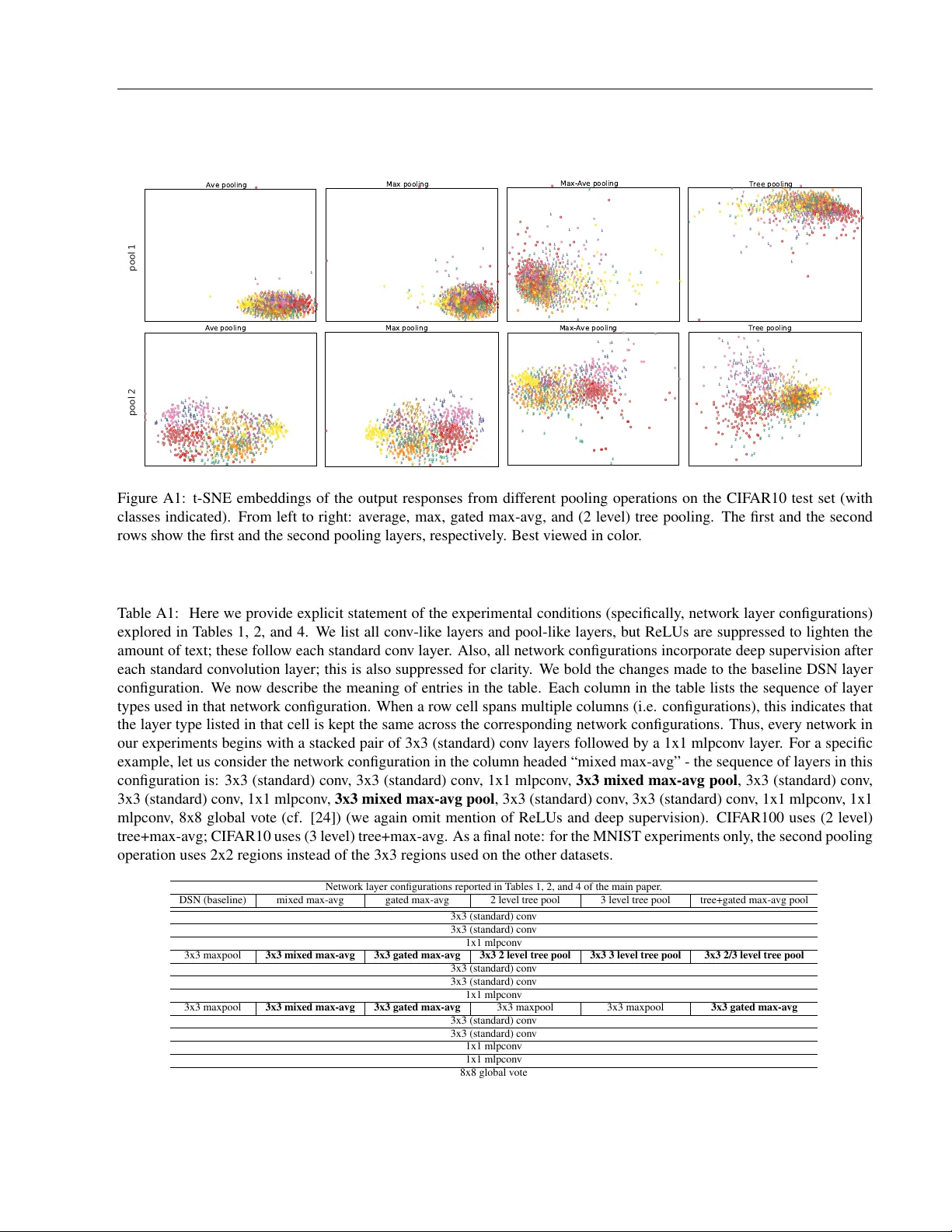
Generalizing P ooling Functions in Con volutional Neural Netw orks: Mixed, Gated, and T r ee Chen-Y u Lee Patrick W . Gallagher Zhuo wen T u UCSD ECE UCSD Cognitiv e Science UCSD Cognitiv e Science chl260@ucsd.edu patrick.w.gallagher@gmail.com ztu@ucsd.edu Abstract W e seek to improv e deep neural networks by generalizing the pooling operations that play a central role in current architectures. W e pursue a careful exploration of approaches to allow pool- ing to learn and to adapt to complex and vari- able patterns. The two primary directions lie in (1) learning a pooling function via (two strate- gies of) combining of max and av erage pooling, and (2) learning a pooling function in the form of a tree-structured fusion of pooling filters that are themselves learned. In our experiments ev- ery generalized pooling operation we explore im- prov es performance when used in place of av er- age or max pooling. W e experimentally demon- strate that the proposed pooling operations pro- vide a boost in in variance properties relative to con ventional pooling and set the state of the art on sev eral widely adopted benchmark datasets; they are also easy to implement, and can be ap- plied within various deep neural network archi- tectures. These benefits come with only a light increase in computational o verhead during train- ing and a very modest increase in the number of model parameters. 1 Introduction The recent resurgence of neurally-inspired systems such as deep belief nets (DBN) [10], con volutional neural net- works (CNNs) [18], and the sum-and-max infrastructure [32] has deri ved significant benefit from building more so- phisticated network structures [38, 33] and from bringing learning to non-linear activations [6, 24]. The pooling op- eration has also played a central role, contributing to in- variance to data v ariation and perturbation. Howe ver , pool- ing operations have been little revised beyond the current primary options of av erage, max, and stochastic pooling Patent disclosure, UCSD Docket No. SD2015-184, “Forest Con- volutional Neural Network”, filed on March 4, 2015. UCSD Docket No. SD2016-053, “Generalizing Pooling Functions in Con volutional Neural Network”, filed on Sept 23, 2015 [3, 40]; this despite indications that e.g. choosing from more than just one type of pooling operation can benefit performance [31]. In this paper , we desire to bring learning and “responsive- ness” (i.e., to characteristics of the region being pooled) into the pooling operation. V arious approaches are possi- ble, but here we pursue two in particular . In the first ap- proach, we consider combining typical pooling operations (specifically , max pooling and av erage pooling); within this approach we further in vestigate two strategies by which to combine these operations. One of the strategies is “unre- sponsiv e”; for reasons discussed later, we call this strat- egy mixed max-average pooling . The other strategy is “re- sponsiv e”; we call this strategy gated max-averag e pooling , where the ability to be responsiv e is provided by a “gate” in analogy to the usage of gates elsewhere in deep learning. Another natural generalization of pooling operations is to allow the pooling operations that are being combined to themselves be learned. Hence in the second approach, we learn to combine pooling filters that are themselves learned. Specifically , the learning is performed within a binary tree (with number of lev els that is pre-specified rather than “grown” as in traditional decision trees) in which each leaf is associated with a learned pooling filter . As we consider internal nodes of the tree, each parent node is associated with an output value that is the mixture of the child node output values, until we finally reach the root node. The root node corresponds to the overall output produced by the tree. W e refer to this strategy as tree pooling . T ree pool- ing is intended (1) to learn pooling filters directly from the data; (2) to learn how to combine leaf node pooling filters in a differentiable f ashion; (3) to bring together these other characteristics within a hierarchical tree structure. When the mixing of the node outputs is allowed to be “re- sponsiv e”, the resulting tree pooling operation becomes an integrated method for learning pooling filters and combi- nations of those filters that are able to display a range of different behaviors depending on the characteristics of the region being pooled. W e pursue experimental v alidation and find that: In the ar- Generalizing Pooling Functions in CNNs: Mixed, Gated, and T ree chitectures we inv estigate, replacing standard pooling oper- ations with any of our proposed generalized pooling meth- ods boosts performance on each of the standard bench- mark datasets, as well as on the lar ger and more com- plex ImageNet dataset. W e attain state-of-the-art results on MNIST , CIF AR10 (with and without data augmenta- tion), and SVHN. Our proposed pooling operations can be used as drop-in replacements for standard pooling opera- tions in various current architectures and can be used in tandem with other performance-boosting approaches such as learning activ ation functions, training with data augmen- tation, or modifying other aspects of network architecture — we confirm improvements when used in a DSN-style architecture, as well as in AlexNet and GoogLeNet. Our proposed pooling operations are also simple to implement, computationally undemanding (ranging from 5% to 15% additional o verhead in timing experiments), dif ferentiable, and use only a modest number of additional parameters. 2 Related W ork In the current deep learning literature, popular pooling functions include max, a verage, and stochastic pooling [3, 2, 40]. A recent effort using more complex pooling op- erations, spatial pyramid pooling [9], is mainly designed to deal with images of varying size, rather than delving in to different pooling functions or incorporating learning. Learning pooling functions is analogous to receptiv e field learning [8, 11, 5, 15]. Howe ver methods like [15] lead to a more difficult learning procedure that in turn leads to a less competitiv e result, e.g. an error rate of 16 . 89% on unaugmented CIF AR10. Since our tree pooling approach in volv es a tree structure in its learning, we observe an analogy to “logic-type” ap- proaches such as decision trees [27] or “logical operators” [25]. Such approaches have played a central role in artifi- cial intelligence for applications that require “discrete” rea- soning, and are often intuitively appealing. Unfortunately , despite the appeal of such logic-type approaches, there is a disconnect between the functioning of decision trees and the functioning of CNNs — the output of a standard de- cision tree is non-continuous with respect to its input (and thus nondifferentiable). This means that a standard deci- sion tree is not able to be used in CNNs, whose learning process is performed by back propagation using gradients of differentiable functions. Part of what allows us to pur- sue our approaches is that we ensure the resulting pooling operation is differentiable and thus usable within network backpropagation. A recent work, referred to as auto-encoder trees [13], also pays attention to a differentiable use of tree structures in deep learning, but is distinct from our method as it focuses on learning encoding and decoding methods (rather than pooling methods) using a “soft” decision tree for a genera- tiv e model. In the supervised setting, [4] incorporates mul- tilayer perceptrons within decision trees, but simply uses trained perceptrons as splitting nodes in a decision forest; not only does this result in training processes that are sep- arate (and thus more difficult to train than an integrated training process), this training process does not in volv e the learning of any pooling filters. 3 Generalizing Pooling Operations A typical con volutional neural network is structured as a series of con volutional layers and pooling layers. Each con- volutional layer is intended to produce representations (in the form of activ ation values) that reflect aspects of local spatial structures, and to consider multiple channels when doing so. More specifically , a con volution layer computes “feature response maps” that in volve multiple channels within some localized spatial region. On the other hand, a pooling layer is restricted to act within just one channel at a time, “condensing” the activ ation values in each spatially- local region in the currently considered channel. An early reference related to pooling operations (although not ex- plicitly using the term “pooling”) can be found in [11]. In modern visual recognition systems, pooling operations play a role in producing “downstream” representations that are more robust to the effects of variations in data while still preserving important motifs. The specific choices of av erage pooling [18, 19] and max pooling [28] hav e been widely used in many CNN-like architectures; [3] includes a theoretical analysis (albeit one based on assumptions that do not hold here). Our goal is to bring learning and “responsiv eness” into the pooling operation. W e focus on two approaches in particular . In the first approach, we begin with the (con- ventional, non-learned) pooling operations of max pooling and average pooling and learn to combine them. W ithin this approach, we further consider two strategies by which to combine these fixed pooling operations. One of these strategies is “unresponsi ve” to the characteristics of the re- gion being pooled; the learning process in this strategy will result in an effecti ve pooling operation that is some spe- cific, unchanging “mixture” of max and average. T o em- phasize this unchanging mixture, we refer to this strategy as mixed max-averag e pooling . The other strategy is “responsiv e” to the characteristics of the region being pooled; the learning process in this strat- egy results in a “gating mask”. This learned gating mask is then used to determine a “responsi ve” mix of max pool- ing and a verage pooling; specifically , the v alue of the inner product between the gating mask and the current region be- ing pooled is fed through a sigmoid, the output of which is used as the mixing proportion between max and average. T o emphasize the role of the gating mask in determining the “responsive” mixing proportion, we refer to this strat- egy as gated max-aver age pooling . Both the mixed strategy and the gated strategy inv olve com- binations of fixed pooling operations; a complementary Chen-Y u Lee, Patrick W . Gallagher , Zhuowen T u generalization to these strategies is to learn the pooling op- erations themselves. From this, we are in turn led to con- sider learning pooling operations and also learning to com- bine those pooling operations. Since these combinations can be considered within the context of a binary tree struc- ture, we refer to this approach as tree pooling . W e pursue further details in the following sections. 3.1 Combining max and av erage pooling functions 3.1.1 “Mixed” max-av erage pooling The con ventional pooling operation is fixed to be either a simple av erage f ave ( x ) = 1 N P N i =1 x i or a maximum oper- ation f max ( x ) = max i x i , where the vector x contains the activ ation values from a local pooling region of N pixels (typical pooling region dimensions are 2 × 2 or 3 × 3 ) in an image or a channel. At present, max pooling is often used as the default in CNNs. W e touch on the relati ve performance of max pool- ing and, e.g., a verage pooling as part of a collection of exploratory experiments to test the in v ariance properties of pooling functions under common image transformations (including rotation, translation, and scaling); see Figure 2. The results indicate that, on the evaluation dataset, there are regimes in which either max pooling or av erage pool- ing demonstrates better performance than the other (al- though we observe that both of these choices are outper- formed by our proposed pooling operations). In the light of observation that neither max pooling nor av erage pool- ing dominates the other , a first natural generalization is the strategy we call “mixed” max-av erage pooling, in which we learn specific mixing proportion parameters from the data. When learning such mixing proportion parameters one has several options (listed in order of increasing num- ber of parameters): learning one mixing proportion param- eter (a) per net, (b) per layer , (c) per layer/region being pooled (but used for all channels across that region), (d) per layer/channel (but used for all re gions in each channel) (e) per layer/region/channel combination. The form for each “mixed” pooling operation (written here for the “one per layer” option; the expression for other op- tions differs only in the subscript of the mixing proportion a ) is: f mix ( x ) = a ` · f max ( x ) + (1 − a ` ) · f avg ( x ) (1) where a ` ∈ [0 , 1] is a scalar mixing proportion specify- ing the specific combination of max and a verage; the sub- script ` is used to indicate that this equation is for the “one per layer” option. Once the output loss function E is de- fined, we can automatically learn each mixing proportion a (where we no w suppress any subscript specifying which of the options we choose). V anilla backpropagation for this learning is giv en by ∂ E ∂ a = ∂ E ∂ f mix ( x ) ∂ f mix ( x ) ∂ a = δ (max i x i − 1 N N X i =1 x i ) , (2) where δ = ∂ E /∂ f mix ( x ) is the error backpropagated from the following layer . Since pooling operations are typically placed in the midst of a deep neural network, we also need (a) (b) (c) Figure 1: Illustration of proposed pooling operations: (a) mixed max-average pooling, (b) gated max-average pool- ing, and (c) Tree pooling (3 lev els in this figure). W e indi- cate the region being pooled by x , gating masks by ω , and pooling filters by v (subscripted as appropriate). to compute the error signal to be propagated back to the previous layer: ∂ E ∂ x i = ∂ E ∂ f mix ( x i ) ∂ f mix ( x i ) ∂ x i (3) = δ  a · 1 [ x i = max i x i ] + (1 − a ) · 1 N  , (4) where 1 [ · ] denotes the 0 / 1 indicator function. In the ex- periment section, we report results for the “one parameter per pooling layer” option; the network for this experiment has 2 pooling layers and so has 2 more parameters than a network using standard pooling operations. W e found that ev en this simple option yielded a surprisingly large performance boost. W e also obtain results for a simple 50/50 mix of max and av erage, as well as for the option with the largest number of parameters: one parameter for each combination of layer/channel/re gion, or pc × ph × pw parameters for each “mixed” pooling layer using this op- tion (where pc is the number of channels being pooled by the pooling layer , and the number of spatial regions be- ing pooled in each channel is ph × pw ). W e observe that the increase in the number of parameters is not met with a corresponding boost in performance, and so we pursue the “one per layer” option. 3.1.2 “Gated” max-av erage pooling In the previous section we considered a strategy that we referred to as “mixed” max-average pooling; in that strat- Generalizing Pooling Functions in CNNs: Mixed, Gated, and T ree egy we learned a mixing proportion to be used in combin- ing max pooling and average pooling. As mentioned ear- lier , once learned, each mixing proportion a remains fixed — it is “nonresponsiv e” insofar as it remains the same no matter what characteristics are present in the region being pooled. W e now consider a “responsive” strategy that we call “gated” max-average pooling. In this strategy , rather than directly learning a mixing proportion that will be fix ed after learning, we instead learn a “gating mask” (with spa- tial dimensions matching that of the re gions being pooled). The scalar result of the inner product between the gating mask and the region being pooled is fed through a sigmoid to produce the v alue that we use as the mixing proportion. This strategy means that the actual mixing proportion can vary during use depending on characteristics present in the region being pooled. T o be more specific, suppose we use x to denote the v alues in the region being pooled and ω to denote the values in a “gating mask”. The “respon- siv e” mixing proportion is then giv en by σ ( ω | x ) , where σ ( ω | x ) = 1 / (1 + exp {− ω | x } ) ∈ [0 , 1] is a sigmoid func- tion. Analogously to the strategy of learning mixing proportion parameter , when learning gating masks one has sev eral op- tions (listed in order of increasing number of parameters): learning one gating mask (a) per net, (b) per layer , (c) per layer/region being pooled (but used for all channels across that region), (d) per layer/channel (but used for all regions in each channel) (e) per layer/region/channel com- bination. W e suppress the subscript denoting the specific option, since the equations are otherwise identical for each option. The resulting pooling operation for this “gated” max- av erage pooling is: f gate ( x ) = σ ( ω | x ) f max ( x ) + (1 − σ ( ω | x )) f avg ( x ) (5) W e can compute the gradient with respect to the internal “gating mask” ω using the same procedure considered pre- viously , yielding ∂ E ∂ ω = ∂ E ∂ f gate ( x ) ∂ f gate ( x ) ∂ ω (6) = δ σ ( ω | x )(1 − σ ( ω | x )) x (max i x i − 1 N N X i =1 x i ) , (7) and ∂ E ∂ x i = ∂ E ∂ f gate ( x i ) ∂ f gate ( x i ) ∂ x i (8) = δ  σ ( ω | x )(1 − σ ( ω | x )) ω i (max i x i − 1 N N X i =1 x i ) (9) + σ ( ω | x ) · 1 [ x i = max i x i ] + (1 − σ ( ω | x )) 1 N  . In a head-to-head parameter count, ev ery single mixing proportion parameter a in the “mixed” max-a verage pool- ing strategy corresponds to a gating mask ω in the “gated” strategy (assuming the y use the same parameter count op- tion). T o take a specific example, suppose that we con- sider a network with 2 pooling layers and pooling regions that are 3 × 3 . If we use the “mixed” strategy and the per-layer option, we would hav e a total of 2 = 2 × 1 extra parameters relative to standard pooling. If we use the “gated” strategy and the per-layer option, we would hav e a total of 18 = 2 × 9 extra parameters, where 9 is the number of parameters in each gating mask. The “mixed” strategy detailed immediately above uses fewer parameters and is “nonresponsiv e”; the “gated” strate gy in- volv es more parameters and is “responsiv e”. In our exper - iments, we find that “mixed” (with one mix per pooling layer) is outperformed by “gated” with one gate per pool- ing layer . Interestingly , an 18 parameter “gated” network with only one gate per pooling layer also outperforms a “mixed” option with far more parameters ( 40 , 960 with one mix per layer/channel/region) — except on the relativ ely large SVHN dataset. W e touch on this below; Section 5 contains details. 3.1.3 Quick comparison: mixed and gated pooling The results in T able 1 indicate the benefit of learning pool- ing operations over not learning. W ithin learned pooling operations, we see that when the number of parameters in the mixed strategy is increased, performance improv es; howe ver , parameter count is not the entire story . W e see that the “responsive” gated max-avg strategy consistently yields better performance (using 18 extra parameters) than is achiev ed with the > 40k extra parameters in the 1 per layer/rg/ch “non-responsi ve” mixed max-avg strategy . The relativ ely larger SVHN dataset pro vides the sole excep- tion (SVHN has ≈ 600k training images versus ≈ 50k for MNIST , CIF AR10, and CIF AR100) — we found baseline 1.91%, 50/50 mix 1.84%, mixed (1 per lyr) 1.76%, mixed (1 per lyr/ch/rg) 1.64%, and gated (1 per lyr) 1.74%. T able 1: Classification error (in %) comparison between baseline model (trained with con ventional max pooling) and corresponding networks in which max pooling is re- placed by the pooling operation listed. A superscripted + indicates the standard data augmentation as in [24, 21, 34]. W e report means and standard deviations over 3 separate trials without model av eraging. Method MNIST CIF AR10 CIF AR10 + CIF AR100 Baseline 0.39 9.10 7.32 34.21 w/ Stochastic no learning 0.38 ± 0.04 8.50 ± 0.05 7.30 ± 0.07 33.48 ± 0.27 w/ 50/50 mix no learning 0.34 ± 0.012 8.11 ± 0.10 6.78 ± 0.17 33.53 ± 0.16 w/ Mixed 1 per pool layer 2 extra params 0.33 ± 0.018 8.09 ± 0.19 6.62 ± 0.21 33.51 ± 0.11 w/ Mixed 1 per layer/ch/rg > 40k extra params 0.30 ± 0.012 8.05 ± 0.16 6.58 ± 0.30 33.35 ± 0.19 w/ Gated 1 per pool layer 18 extra params 0.29 ± 0.016 7.90 ± 0.07 6.36 ± 0.28 33.22 ± 0.16 3.2 T r ee pooling The strategies described above each inv olve combinations of fixed pooling operations; another natural generalization Chen-Y u Lee, Patrick W . Gallagher , Zhuowen T u of pooling operations is to allow the pooling operations that are being combined to themselves be learned. These pool- ing layers remain distinct from con volution layers since pooling is performed separately within each channel; this channel isolation also means that e ven the option that intro- duces the lar gest number of parameters still introduces far fewer parameters than a con volution layer would introduce. The most basic version of this approach would not in volve combining learned pooling operations, but simply learning pooling operations in the form of the v alues in pooling fil- ters. One step further brings us to what we refer to as tr ee pooling , in which we learn pooling filters and also learn to responsiv ely combine those learned filters. Both aspects of this learning are performed within a binary tree (with number of levels that is pre-specified rather than “grown” as in traditional decision trees) in which each leaf is associated with a pooling filter learned during training. As we consider internal nodes of the tree, each parent node is associated with an output value that is the mixture of the child node output values, until we finally reach the root node. The root node corresponds to the overall output pro- duced by the tree and each of the mixtures (by which child outputs are “fused” into a parent output) is responsiv ely learned. T ree pooling is intended (1) to learn pooling filters directly from the data; (2) to learn how to “mix” leaf node pooling filters in a differentiable fashion; (3) to bring to- gether these other characteristics within a hierarchical tree structure. Each leaf node in our tree is associated with a “pooling filter” that will be learned; for a node with index m , we denote the pooling filter by v m ∈ R N . If we had a “degen- erate tree” consisting of only a single (leaf) node, pooling a region x ∈ R N would result in the scalar value v | m x . For (internal) nodes (at which two child values are com- bined into a single parent value), we proceed in a fashion analogous to the case of gated max-average pooling, with learned “gating masks” denoted (for an internal node m ) by ω m ∈ R N . The “pooling result” at any arbitrary node m is thus f m ( x ) = ( v | m x if leaf node σ ( ω | m x ) f m, left ( x ) + (1 − σ ( ω | m x )) f m, right ( x ) if internal node (10) The overall pooling operation would thus be the result of ev aluating f root node ( x ) . The appeal of this tree pooling approach would be limited if one could not train the pro- posed layer in a fashion that was integrated within the net- work as a whole. This would be the case if we attempted to directly use a traditional decision tree, since its output presents points of discontinuity with respect to its inputs. The reason for the discontinuity (with respect to input) of traditional decision tree output is that a decision tree mak es “hard” decisions; in the terminology we have used above, a “hard” decision node corresponds to a mixing propor- tion that can only take on the value 0 or 1 . The conse- quence is that this type of “hard” function is not dif feren- tiable (nor even continuous with respect to its inputs), and this in turn interferes with any ability to use it in iterative parameter updates during backpropagation. This moti vates us to instead use the internal node sigmoid “gate” func- tion σ ( ω | m x ) ∈ [0 , 1] so that the tree pooling function as a whole will be differentiable with respect to its parameters and its inputs. For the specific case of a “2 lev el” tree (with leaf nodes “1” and “2” and internal node “3”) pooling function f tree ( x ) = σ ( ω | 3 x ) v | 1 x + (1 − σ ( ω | 3 x )) v | 2 x , we can use the chain rule to compute the gradients with respect to the leaf node pool- ing filters v 1 , v 2 and the internal node gating mask ω 3 : ∂ E ∂ v 1 = ∂ E ∂ f tree ( x ) ∂ f tree ( x ) ∂ v 1 = δ σ ( ω | 3 x ) x (11) ∂ E ∂ v 2 = ∂ E ∂ f tree ( x ) ∂ f tree ( x ) ∂ v 2 = δ (1 − σ ( ω | 3 x )) x (12) ∂ E ∂ ω 3 = ∂ E ∂ f tree ( x ) ∂ f tree ( x ) ∂ ω 3 = δ σ ( ω | 3 x )(1 − σ ( ω | 3 x )) x ( v | 1 − v | 2 ) x (13) The error signal to be propagated back to the pre vious layer is ∂ E ∂ x = ∂ E ∂ f tree ( x ) ∂ f tree ( x ) ∂ x (14) = δ [ σ ( ω | 3 x )(1 − σ ( ω | 3 x )) ω 3 ( v | 1 − v | 2 ) x (15) + σ ( ω | 3 x ) v 1 + (1 − σ ( ω | 3 x )) v 2 ] 3.2.1 Quick comparison: tree pooling T able 2 collects results related to tree pooling. W e observe that on all datasets but the comparatively simple MNIST , adding a lev el to the tree pooling operation improves per- formance. Ho wev er , ev en further benefit is obtained from the use of tree pooling in the first pooling layer and gated max-avg in the second. T able 2: Classification error (in %) comparison between our baseline model (trained with con ventional max pool- ing) and proposed methods in volving tree pooling. A su- perscripted + indicates the standard data augmentation as in [24, 21, 34]. Method MNIST CIF AR10 CIF AR10 + CIF AR100 SVHN Our baseline 0.39 9.10 7.32 34.21 1.91 T r ee 2 level; 1 per pool layer 0.35 8.25 6.88 33.53 1.80 T r ee 3 level; 1 per pool layer 0.37 8.22 6.67 33.13 1.70 T r ee+Max-A vg 1 per pool layer 0.31 7.62 6.05 32.37 1.69 Comparison with making the network deeper using con v layers T o further in vestigate whether simply adding depth to our baseline network giv es a performance boost comparable to that observed for our proposed pooling op- erations, we report in T able 3 belo w some additional ex- periments on CIF AR10 (error rate in percent; no data aug- mentation). If we count depth by counting any layer with learned parameters as an extra layer of depth (even if there is only 1 parameter), the number of parameter layers in a baseline network with 2 additional standard con volution layers matches the number of parameter layers in our best performing net (although the con volution layers contain many more parameters). Generalizing Pooling Functions in CNNs: Mixed, Gated, and T ree −40 −20 0 20 40 50 62.5 75 87.5 Rotation angle (degrees) Accuracy (%) Max−Ave pooling (ours) Tree pooling (ours) Max pooling Average pooling −8 −4 0 4 8 70 76.25 82.5 88.75 95 Translation (pixels) Accuracy (%) Max−Ave pooling (ours) Tree pooling (ours) Max pooling Average pooling 0.6 0.8 1 1.2 1.4 40 55 70 85 Scale multiplier Accuracy (%) Max−Ave pooling (ours) Tree pooling (ours) Max pooling Average pooling Figure 2: Controlled experiment on CIF AR10 inv estigating the relative benefit of selected pooling operations in terms of robustness to three types of data v ariation. The three kinds of variations we choose to in vestigate are rotation, translation, and scale. W ith each kind of v ariation, we modify the CIF AR10 test images according to the listed amount. W e observe that, across all types and amounts of variation (except extreme down-scaling) the proposed pooling operations in vestigated here (gated max-avg and 2 level tree pooling) provide impro ved rob ustness to these transformations, relativ e to the standard choices of maxpool or avgpool. Our method requires only 72 extra parameters and obtains state-of-the-art 7 . 62% error . On the other hand, making networks deeper with con v layers adds many more param- eters but yields test error that does not drop below 9 . 08% in the configuration explored. Since we follow each ad- ditional con v layer with a ReLU, these networks corre- spond to increasing nonlinearity as well as adding depth and adding (man y) parameters. These experiments in- dicate that the performance of our proposed pooling is not accounted for as a simple effect of the addition of depth/parameters/nonlinearity . T able 3: Classification error (%) on CIF AR10 (without data augmentation) comparison between networks made deeper with standard conv olution layers and proposed T ree+(gated) Max-A vg pooling. Method % Error Extra parameters Baseline 9.10 0 w/ 1 extra con v layer (+ReLU) 9.08 0.6M w/ 2 extra con v layers (+ReLU) 9.17 1.2M w/ T ree+(gated) Max-A vg 7.62 72 Comparison with alternativ e pooling layers T o see whether we might find similar performance boosts by re- placing the max pooling in the baseline network configu- ration with alternati ve pooling operations such as stochas- tic pooling, “pooling” using a stride 2 con volution layer as pooling (cf All-CNN), or a simple fixed 50/50 proportion in max-avg pooling, we performed another set of experiments on unaugmented CIF AR10. From the baseline error rate of 9.10%, replacing each of the 2 max pooling layers with stacked stride 2 conv:ReLU (as in [34]) lo wers the error to 8.77%, but adds 0.5M extra parameters. Using stochastic pooling [40] adds computational ov erhead but no parame- ters and results in 8.50% error . A simple 50/50 mix of max and average is computationally light and yields 8.07% er- ror with no additional parameters. Finally , our tree+gated max-avg configuration adds 72 parameters and achieves a state-of-the-art 7.62% error . 4 Quick Perf ormance Overview For ease of discussion, we collect here observations from subsequent experiments with a view to highlighting aspects that shed light on the performance characteristics of our proposed pooling functions. First, as seen in the experiment shown in Figure 2 replac- ing standard pooling operations with either gated max-avg or (2 level) tree pooling (each using the “one per layer” option) yielded a boost (relativ e to max or avg pooling) in CIF AR10 test accuracy as the test images underwent three different kinds of transformations. This boost was observed across the entire range of transformation amounts for each of the transformations (with the exception of ex- treme downscaling). W e already observe improved ro- bustness in this initial experiment and intend to in vestigate more instances of our proposed pooling operations as time permits. Second, the performance that we attain in the experiments reported in Figure 2, T able 1, T able 2, T able 4, and T able 5 is achieved with very modest additional numbers of param- eters — e.g. on CIF AR10, our best performance (obtained with the tree+gated max-avg configuration) only uses an additional 72 parameters (abov e the 1.8M of our baseline network) and yet reduces test error from 9 . 10% to 7 . 62% ; see the CIF AR10 Section for details. In our AlexNet ex- periment, replacing the maxpool layers with our proposed pooling operations gav e a 6% relative reduction in test er - ror (top-5, single-view) with only 45 additional parame- ters (abov e the > 50M of standard AlexNet); see the Im- ageNet 2012 Section for details. W e also in vestigate the additional time incurred when using our proposed pooling operations; in the experiments reported in the Timing sec- tion, this ov erhead ranges from 5% to 15% . T esting in variance properties Before going to the overall classification results, we in vestigate the in variance proper- ties of networks utilizing either standard pooling operations (max and av erage) or two instances of our proposed pool- ing operations (gated max-avg and 2 le vel tree, each using Chen-Y u Lee, Patrick W . Gallagher , Zhuowen T u the “1 per pool layer” option) that we find to yield best per- formance (see Sec. 5 for architecture details used across each network). W e begin by training four different net- works on the CIF AR10 training set, one for each of the four pooling operations selected for consideration; train- ing details are found in Sec. 5. W e seek to determine the respectiv e in variance properties of these networks by ev al- uating their accuracy on various transformed versions of the CIF AR10 test set. Figure 2 illustrates the test accuracy attained in the presence of image rotation, (vertical) trans- lation, and scaling of the CIF AR10 test set. Timing In order to ev aluate how much additional time is incurred by the use of our proposed learned pooling oper- ations, we measured the av erage forward+backward time per CIF AR10 image. In each case, the one per layer op- tion is used. W e find that the additional computation time incurred ranges from 5% to 15% . More specifically , the baseline network took 3.90 ms; baseline with mixed max- avg took 4.10 ms; baseline with gated max-avg took 4.16 ms; baseline with 2 level tree pooling took 4.25 ms; finally , baseline with tree+gated max-avg took 4.46 ms. 5 Experiments W e ev aluate the proposed max-average pooling and tree pooling approaches on five standard benchmark datasets: MNIST [20], CIF AR10 [16], CIF AR100 [16], SVHN [26] and ImageNet [30]. T o control for the ef fect of differences in data or data preparation, we match our data and data preparation to that used in [21]. Please refer to [21] for the detailed description. W e now describe the basic network architecture and then will specify the v arious hyperparameter choices. The basic experiment architecture contains six 3 × 3 standard con- volutional layers (named conv1 to con v6) and three mlp- con v layers (named mlpcon v1 to mlpcon v3) [24], placed after con v2, conv4, and conv6, respectively . W e chose the number of channels at each layer to be analogous to the choices in [24, 21]; the specific numbers are provided in the sections for each dataset. W e follow e very one of these con v-type layers with ReLU acti vation functions. One final mlpcon v layer (mlpcon v4) is used to reduce the dimension of the last layer to match the total number of classes for each different dataset, as in [24]. The ov erall model has parameter count analogous to [24, 21]. The proposed max- av erage pooling and tree pooling layers with 3 × 3 pooling regions are used after mlpcon v1 and mlpcon v2 layers 1 . W e provide a detailed listing of the network configurations in T able A1 in the Supplementary Materials. Moving on to the hyperparameter settings, dropout with rate 0 . 5 is used after each pooling layer . W e also use hidden layer supervision to ease the training process as 1 There is one exception: on the very small images of the MNIST dataset, the second pooling layer uses 2 × 2 pooling re- gions. in [21]. The learning rate is decreased whene ver the validation error stops decreasing; we use the schedule { 0 . 025 , 0 . 0125 , 0 . 0001 } for all experiments. The momen- tum of 0 . 9 and weight decay of 0 . 0005 are fixed for all datasets as another regularizer besides dropout. All the ini- tial pooling filters and pooling masks ha ve values sampled from a Gaussian distribution with zero mean and standard deviation 0 . 5 . W e use these hyperparameter settings for all experiments reported in T ables 1, 2, and 3. No model a ver- aging is done at test time. 5.1 Classification results T ables 1 and 2 show our overall experimental results. Our baseline is a network trained with conv entional max pool- ing. Mixed refers to the same network but with a max-a vg pooling strategy in both the first and second pooling layers (both using the mixed strategy); Gated has a correspond- ing meaning. T ree (with specific number of lev els noted below) refers to the same again, but with our tree pooling in the first pooling layer only; we do not see further im- prov ement when tree pooling is used for both pooling lay- ers. This observation motiv ated us to consider following a tree pooling layer with a gated max-avg pooling layer: T r ee+Max-A vera ge refers to a network configuration with (2 lev el) tree pooling for the first pooling layer and gated max-av erage pooling for the second pooling layer . All re- sults are produced from the same network structure and hy- perparameter settings — the only difference is in the choice of pooling function. See T able A1 for details. MNIST Our MNIST model has { 128 , 128 , 192 , 192 , 256 , 256 } channels for con v1 to con v6 and { 128 , 192 , 256 } channels for mlpcon v1 to mlpcon v3, respectiv ely . Our only preprocessing is mean subtraction. T ables 4,1, and 2 show previous best results and those for our proposed pooling methods. CIF AR10 Our CIF AR10 model has { 128 , 128 , 192 , 192 , 256 , 256 } channels for con v1 to con v6 and { 128 , 192 , 256 } channels for mlpcon v1 to mlpcon v3, respectiv ely . W e also performed an experiment in which we learned a single pooling filter without the tree structure (i.e., a singleton leaf node containing 9 parameters; one such singleton leaf node per pooling layer) and obtained 0 . 3% improvement over the baseline model. Our results indicate that performance improv es when the pooling filter is learned, and further im- prov es when we also learn ho w to combine learned pooling filters. The All-CNN method in [34] uses con volutional layers in place of pooling layers in a CNN-type network archi- tecture. Howe ver , a standard con volutional layer requires many more parameters than a gated max-average pooling layer (only 9 parameters for a 3 × 3 pooling region ker- nel size in the 1 per pooling layer option) or a tree-pooling layer ( 27 parameters for a 2 lev el tree and 3 × 3 pooling region kernel size, again in the 1 per pooling layer option). The pooling operations in our tree+max-avg network con- Generalizing Pooling Functions in CNNs: Mixed, Gated, and T ree T able 4: Classification error (in %) reported by recent com- parable publications on four benchmark datasets with a sin- gle model and no data augmentation, unless otherwise in- dicated. A superscripted + indicates the standard data aug- mentation as in [24, 21, 34]. A “-” indicates that the cited work did not report results for that dataset. A fix ed network configuration using the proposed tree+max-avg pooling (1 per pool layer option) yields state-of-the-art performance on all datasets (with the exception of CIF AR100). Method MNIST CIF AR10 CIF AR10 + CIF AR100 SVHN CNN [14] 0.53 - - - - Stoch. Pooling [40] 0.47 15.13 - 42.51 2.80 Maxout Networks [6] 0.45 11.68 9.38 38.57 2.47 Prob. Maxout [35] - 11.35 9.39 38.14 2.39 Tree Priors [36] - - - 36.85 - DropConnect [22] 0.57 9.41 9.32 - 1.94 FitNet [29] 0.51 - 8.39 35.04 2.42 NiN [24] 0.47 10.41 8.81 35.68 2.35 DSN [21] 0.39 9.69 7.97 34.57 1.92 NiN + LA units [1] - 9.59 7.51 34.40 - dasNet [37] - 9.22 - 33.78 - All-CNN [34] - 9.08 7.25 33.71 - R-CNN [23] 0.31 8.69 7.09 31.75 1.77 Our baseline 0.39 9.10 7.32 34.21 1.91 Our Tree+Max-A vg 0.31 7.62 6.05 32.37 1.69 figuration use 7 × 9 = 63 parameters for the (first, 3 lev el) tree-pooling layer — 4 leaf nodes and 3 internal nodes — and 9 parameters in the gating mask used for the (second) gated max-av erage pooling layer , while the best result in [34] contains a total of nearly 500 , 000 parameters in lay- ers performing “pooling like” operations; the relativ e CI- F AR10 accuracies are 7 . 62% (ours) and 9 . 08% (All-CNN). For the data augmentation experiment, we followed the standard data augmentation procedure [24, 21, 34]. When training with augmented data, we observe the same trends seen in the “no data augmentation” experiments. W e note that [7] reports a 4 . 5% error rate with extensi ve data augmentation (including translations, rotations, reflections, stretching, and shearing operations) in a much wider and deeper 50 million parameter network — 28 times more than are in our networks. CIF AR100 Our CIF AR100 model has 192 channels for all con volutional layers and { 96 , 192 , 192 } channels for mlp- con v1 to mlpconv3, respecti vely . Street view house numbers Our SVHN model has { 128 , 128 , 320 , 320 , 384 , 384 } channels for con v1 to conv6 and { 96 , 256 , 256 } channels for mlpcon v1 to mlpcon v3, re- spectiv ely . In terms of amount of data, SVHN has a larger training data set ( > 600k versus the ≈ 50k of most of the other benchmark datasets). The much larger amount of training data motiv ated us to explore what per- formance we might observ e if we pursued the one per layer/channel/region option, which even for the simple mixed max-avg strategy results in a huge increase in total the number of parameters to learn in our proposed pooling layers: specifically , from a total of 2 in the mixed max-a vg strategy , 1 parameter per pooling layer option, we increase to 40,960. Using this one per layer/channel/re gion option for the mixed max-avg strategy , we observe test error (in % ) of 0.30 on MNIST , 8.02 on CIF AR10, 6.61 on CIF AR10 + , 33.27 on CIF AR100, and 1.64 on SVHN. Interestingly , for MNIST , CIF AR10 + , and CIF AR100 this mixed max-avg (1 per layer/channel/re gion) performance is between mix ed max-avg (1 per layer) and gated max-avg (1 per layer); on CIF AR10 mixed max-avg (1 per layer/channel/region) is worse than either of the 1 per layer max-avg strate- gies. The SVHN result using mixed max-avg (1 per layer/channel/region) sets a ne w state of the art. ImageNet 2012 In this e xperiment we do not directly com- pete with the best performing result in the challenge (since the winning methods [38] in volve many additional aspects beyond pooling operations), b ut rather to provide an il- lustrativ e comparison of the relati ve benefit of the pro- posed pooling methods versus conv entional max pooling on this dataset. W e use the same network structure and parameter setup as in [17] (no hidden layer supervision) but simply replace the first max pooling with the (pro- posed 2 le vel) tree pooling (2 leaf nodes and 1 internal node for 27 = 3 × 9 parameters) and replace the second and third max pooling with gated max-average pooling (2 gating masks for 18 = 2 × 9 parameters). Relativ e to the original AlexNet, this adds 45 more parameters (over the > 50M in the original) and achie ves relativ e error reduction of 6% (for top-5, single-view) and 5% (for top-5, multi- view). Our GoogLeNet configuration uses 4 gated max-avg pooling layers, for a total of 36 extra parameters ov er the 6.8 million in standard GoogLeNet. T able 5 shows a di- rect comparison (in each case we use single net predictions rather than ensemble). T able 5: ImageNet 2012 test error (in %). BN denotes Batch Normalization [12]. Method top-1 s-view top-5 s-view top-1 m-view top-5 m-view AlexNet [17] 43.1 19.9 40.7 18.2 AlexNet w/ ours 41.4 18.7 39.3 17.3 GoogLeNet [38] - 10.07 - 9.15 GoogLeNet w/ BN 28.68 9.53 27.81 9.09 GoogLeNet w/ BN + ours 28.02 9.16 27.60 8.93 6 Observations fr om Experiments In each experiment, using any of our proposed pooling operations boosted performance. A fixed network con- figuration using the proposed tree+max-a vg pooling (1 per pool layer option) yields state-of-the-art performance on MNIST , CIF AR10 (with and without data augmenta- tion), and SVHN. W e observ ed boosts in tandem with data augmentation, multi-vie w predictions, batch normal- ization, and se veral different architectures — NiN-style, DSN-style, the > 50M parameter Ale xNet, and the 22-layer GoogLeNet. Chen-Y u Lee, Patrick W . Gallagher , Zhuowen T u Acknowledgment This work is supported by NSF awards IIS-1216528 (IIS-1360566) and IIS-0844566(IIS- 1360568). References [1] F . Agostinelli, M. Hof fman, P . Sadowski, and P . Baldi. Learning activ ation functions to improve deep neural net- works. In ICLR , 2015. [2] Y . Boureau, N. Le Roux, F . Bach, J. Ponce, and Y . LeCun. Ask the locals: multi-way local pooling for image recogni- tion. In ICCV , 2011. [3] Y . Boureau, J. Ponce, and Y . LeCun. A Theoretical Analysis of Feature Pooling in V isual Recognition. In ICML , 2010. [4] S. R. Bulo and P . Kontschieder . Neural Decision Forests for Semantic Image Labelling. In CVPR , 2014. [5] A. Coates and A. Y . Ng. Selecting receptiv e fields in deep networks. In NIPS , 2011. [6] I. J. Goodfellow , D. W arde-F arley , M. Mirza, A. C. Courville, and Y . Bengio. Maxout Networks. In ICML , 2013. [7] B. Graham. Fractional Max-Pooling. arXiv preprint arXiv:1412.6071 , 2014. [8] C. Gulcehre, K. Cho, R. Pascanu, and Y . Bengio. Learned- norm pooling for deep feedforward and recurrent neural net- works. In MLKDD . 2014. [9] K. He, X. Zhang, S. Ren, and J. Sun. Spatial pyramid pool- ing in deep conv olutional networks for visual recognition. In ECCV , 2014. [10] G. Hinton, S. Osindero, and Y .-W . T eh. A fast learning al- gorithm for deep belief nets. Neural Computation , 2006. [11] D. H. Hubel and T . N. Wiesel. Recepti ve fields, binocu- lar interaction and functional architecture in the cat’ s visual cortex. Journal of Physiology , 1962. [12] S. Ioffe and C. Szegedy . Batch normalization: Accelerating deep network training by reducing internal cov ariate shift. arXiv pr eprint arXiv:1502.03167 , 2015. [13] O. Irsoy and E. Alpaydin. Autoencoder T rees. In NIPS Deep Learning W orkshop , 2014. [14] K. Jarrett, K. Kavukcuoglu, M. Ranzato, and Y . LeCun. What is the best multi-stage architecture for object recog- nition? In ICCV , 2009. [15] Y . Jia, C. Huang, and T . Darrell. Beyond spatial pyramids. In CVPR , 2012. [16] A. Krizhevsky . Learning Multiple Layers of Features from T iny Images. CS Dept., U T or onto, T ec h. Rep. , 2009. [17] A. Krizhevsk y , I. Sutskev er, and G. E. Hinton. ImageNet Classification with Deep Conv olutional Neural Networks. In NIPS , 2012. [18] Y . LeCun, B. Boser, J. S. Denker , D. Henderson, R. Ho ward, W . Hubbard, and L. Jackel. Backpropagation applied to handwritten zip code recognition. Neural Computation , 1989. [19] Y . LeCun, L. Bottou, Y . Bengio, and P . Haffner . Gradient- based learning applied to document recognition. In Proceed- ings of the IEEE , 1998. [20] Y . LeCun and C. Cortes. The MNIST database of handwrit- ten digits, 1998. [21] C.-Y . Lee, S. Xie, P . Gallagher , Z. Zhang, and Z. Tu. Deeply- Supervised Nets. In AIST ATS , 2015. [22] W . Li, M. Zeiler , S. Zhang, Y . LeCun, and R. Fergus. Regu- larization of NNs using DropConnect. In ICML , 2013. [23] M. Liang and X. Hu. Recurrent CNNs for Object Recogni- tion. In CVPR , 2015. [24] M. Lin, Q. Chen, and S. Y an. Network in network. In ICLR , 2013. [25] J. Mink er . Logic-Based Artificial Intellig ence . Springer Sci- ence & Business Media, 2000. [26] Y . Netzer , T . W ang, A. Coates, A. Bissacco, B. W u, and A. Y . Ng. Reading Digits in Natural Images with Unsuper- vised Feature Learning. In NIPS W orkshop on Deep Learn- ing and Unsupervised F eatur e Learning , 2011. [27] J. R. Quinlan. C4.5: Pr ogramming for machine learning . 1993. [28] M. Ranzato, Y .-L. Boureau, and Y . LeCun. Sparse Feature Learning for Deep Belief Networks. In NIPS , 2007. [29] A. Romero, N. Ballas, S. E. Kahou, A. Chassang, C. Gatta, and Y . Bengio. FitNets: Hints for Thin Deep Nets. In ICLR , 2015. [30] O. Russako vsky , J. Deng, H. Su, J. Krause, S. Satheesh, S. Ma, Z. Huang, A. Karpathy , A. Khosla, M. Bernstein, A. C. Berg, and L. Fei-Fei. ImageNet Large Scale V isual Recognition Challenge. IJCV , 2014. [31] D. Scherer, A. M ¨ uller , and S. Behnk e. Evaluation of pooling operations in con volutional architectures for object recogni- tion. In ICANN . 2010. [32] T . Serre, L. W olf, S. Bileschi, M. Riesenhuber, and T . Pog- gio. Robust object recognition with corte x-like mechanisms. IEEE TP AMI , 2007. [33] K. Simonyan and A. Zisserman. V ery deep conv olutional networks for lar ge-scale image recognition. In ICLR , 2015. [34] J. T . Springenberg, A. Dosovitskiy , T . Brox, and M. Ried- miller . Striving for Simplicity . In ICLR , 2015. [35] J. T . Springenberg and M. Riedmiller . Improving deep neu- ral networks with probabilistic maxout units. In ICLR , 2014. [36] N. Sriv astava and R. R. Salakhutdinov . Discriminati ve trans- fer learning with tree-based priors. In NIPS , 2013. [37] M. Stollenga, J. Masci, F . J. Gomez, and J. Schmidhuber . Deep Networks with Internal Selecti ve Attention through Feedback Connections. In NIPS , 2014. [38] C. Szegedy , W . Liu, Y . Jia, P . Sermanet, S. Reed, D. Anguelov , D. Erhan, V . V anhoucke, and A. Rabi- novich. Going Deeper with Con volutions. arXiv pr eprint arXiv:1409.4842 , 2014. [39] L. V an der Maaten and G. Hinton. V isualizing data using t-SNE. JMLR , 2008. [40] M. D. Zeiler and R. Fergus. Stochastic Pooling for Regu- larization of Deep Con volutional Neural Networks. arXiv pr eprint arXiv:1301.3557 , 2013. Generalizing Pooling Functions in CNNs: Mixed, Gated, and T ree A1 Supplementary Materials V isualization of network inter nal representations T o gain additional qualitati ve understanding of the pooling methods we are considering, we use the popular t-SNE [39] algorithm to visualize embeddings of some internal feature responses from pooling operations. Specifically , we again use four networks (one utilizing each of the selected types of pooling) trained on the CIF AR10 training set (see Sec. 5 for architecture details used across each network). W e extract feature responses for a randomly chosen 800 -image subset of the CIF AR10 test set at the first (i.e., earlies t) and second pooling layers of each network. These feature re- sponse vectors are then embedded into 2-d using t-SNE; see Figure A1. The first row shows the embeddings of the internal activ a- tions immediately after the first pooling operation; the sec- ond row shows embeddings of acti vations immediately af- ter the second pooling operation. From left to right we plot the t-SNE embeddings of the pooling activ ations within networks that are trained with average, max, gated max- avg, and (2 lev el) tree pooling. W e can see that certain classes such as “0” (airplane), “2” (bird), and “9” (truck) are more separated with the proposed methods than they are with the con ventional av erage and max pooling func- tions. W e can also see that the embeddings of the second- pooling-layer activ ations are generally more separable than the embeddings of first-pooling-layer activ ations. Chen-Y u Lee, Patrick W . Gallagher , Zhuowen T u poo l 1 3 8 8 0 6 6 1 6 3 1 0 9 5 7 9 8 5 7 8 6 7 0 4 9 5 2 4 0 9 6 6 5 4 5 9 2 4 1 9 5 4 6 5 6 0 9 3 9 7 6 9 8 0 3 8 8 7 7 4 6 7 3 6 3 6 2 1 2 3 7 2 6 8 8 0 2 9 3 3 8 8 1 1 7 2 5 2 7 8 9 0 3 8 6 4 6 6 0 0 7 4 5 6 3 1 1 3 6 8 7 4 0 6 2 1 3 0 4 2 7 8 3 1 2 8 0 8 3 5 2 4 1 8 9 1 2 9 7 2 9 6 5 6 3 8 7 6 2 5 2 8 9 6 0 0 5 2 9 5 4 2 1 6 6 8 4 8 4 5 0 9 9 9 8 9 9 3 7 5 0 0 5 2 2 3 8 6 3 4 0 5 8 0 1 7 2 8 8 7 8 5 1 8 7 1 3 0 5 7 9 7 4 5 9 8 0 7 9 8 2 7 6 9 4 3 9 6 4 7 6 5 1 5 8 8 0 4 0 5 5 1 1 8 9 0 3 1 9 2 2 5 3 9 9 4 0 3 0 0 9 8 1 5 7 0 8 2 4 7 0 2 3 6 3 8 5 0 3 4 3 9 0 6 1 0 9 1 0 7 9 1 2 6 9 3 4 6 0 0 6 6 6 3 2 6 1 8 2 1 6 8 6 8 0 4 0 7 7 5 5 3 5 2 3 4 1 7 5 4 6 1 9 3 6 6 9 3 8 0 7 2 6 2 5 8 5 4 6 8 9 9 1 0 2 2 7 3 2 8 0 9 5 8 1 9 4 1 3 8 1 4 7 9 4 2 7 0 7 0 6 6 9 0 9 2 8 7 2 2 5 1 2 6 2 9 6 2 3 0 3 9 8 7 8 8 4 0 1 8 2 7 9 3 6 1 9 0 7 3 7 4 5 0 0 2 9 3 4 0 6 2 5 3 7 3 7 2 5 3 1 1 4 9 9 5 7 5 0 2 2 2 9 7 3 9 4 3 5 4 6 5 6 1 4 3 4 4 3 7 8 3 7 8 0 5 7 6 0 5 4 8 6 8 5 5 9 9 9 5 0 1 0 8 1 1 8 0 2 2 0 4 6 5 4 9 4 7 9 9 4 5 6 6 1 5 3 8 9 5 8 5 7 0 7 0 5 0 0 4 6 9 0 9 5 6 6 6 2 9 0 1 7 6 7 5 9 1 6 2 5 5 5 8 5 9 4 6 4 3 2 0 7 6 2 2 3 9 7 9 2 6 7 1 3 6 6 8 9 7 5 4 0 8 4 0 9 3 4 8 9 6 9 2 6 1 4 7 3 5 3 8 5 0 2 1 6 4 3 3 9 6 9 8 8 5 8 6 6 2 1 7 7 1 2 7 9 9 4 4 1 2 5 6 8 7 6 8 3 0 5 5 3 0 7 9 1 3 4 4 5 3 9 5 6 9 2 1 1 4 1 9 4 7 6 3 8 9 0 1 3 6 3 6 3 2 0 3 1 0 5 9 6 4 8 9 6 9 6 3 0 3 2 2 7 8 3 8 2 7 5 7 2 4 8 7 4 2 9 8 8 6 8 8 7 4 3 3 8 4 9 4 8 8 1 8 2 1 3 6 5 4 2 7 9 9 4 1 4 1 3 2 7 0 7 9 7 6 6 2 5 9 2 9 1 2 2 6 8 2 1 3 6 6 0 1 2 7 0 5 4 6 1 6 4 0 2 2 6 0 5 9 1 7 6 7 0 3 9 6 8 3 0 3 4 7 7 1 4 7 2 Ave pooling 3 8 8 0 6 6 1 6 3 1 0 9 5 7 9 8 5 7 8 6 7 0 4 9 5 2 4 0 9 6 6 5 4 5 9 2 4 1 9 5 4 6 5 6 0 9 3 9 7 6 9 8 0 3 8 8 7 7 4 6 7 3 6 3 6 2 1 2 3 7 2 6 8 8 0 2 9 3 3 8 8 1 1 7 2 5 2 7 8 9 0 3 8 6 4 6 6 0 0 7 4 5 6 3 1 1 3 6 8 7 4 0 6 2 1 3 0 4 2 7 8 3 1 2 8 0 8 3 5 2 4 1 8 9 1 2 9 7 2 9 6 5 6 3 8 7 6 2 5 2 8 9 6 0 0 5 2 9 5 4 2 1 6 6 8 4 8 4 5 0 9 9 9 8 9 9 3 7 5 0 0 5 2 2 3 8 6 3 4 0 5 8 0 1 7 2 8 8 7 8 5 1 8 7 1 3 0 5 7 9 7 4 5 9 8 0 7 9 8 2 7 6 9 4 3 9 6 4 7 6 5 1 5 8 8 0 4 0 5 5 1 1 8 9 0 3 1 9 2 2 5 3 9 9 4 0 3 0 0 9 8 1 5 7 0 8 2 4 7 0 2 3 6 3 8 5 0 3 4 3 9 0 6 1 0 9 1 0 7 9 1 2 6 9 3 4 6 0 0 6 6 6 3 2 6 1 8 2 1 6 8 6 8 0 4 0 7 7 5 5 3 5 2 3 4 1 7 5 4 6 1 9 3 6 6 9 3 8 0 7 2 6 2 5 8 5 4 6 8 9 9 1 0 2 2 7 3 2 8 0 9 5 8 1 9 4 1 3 8 1 4 7 9 4 2 7 0 7 0 6 6 9 0 9 2 8 7 2 2 5 1 2 6 2 9 6 2 3 0 3 9 8 7 8 8 4 0 1 8 2 7 9 3 6 1 9 0 7 3 7 4 5 0 0 2 9 3 4 0 6 2 5 3 7 3 7 2 5 3 1 1 4 9 9 5 7 5 0 2 2 2 9 7 3 9 4 3 5 4 6 5 6 1 4 3 4 4 3 7 8 3 7 8 0 5 7 6 0 5 4 8 6 8 5 5 9 9 9 5 0 1 0 8 1 1 8 0 2 2 0 4 6 5 4 9 4 7 9 9 4 5 6 6 1 5 3 8 9 5 8 5 7 0 7 0 5 0 0 4 6 9 0 9 5 6 6 6 2 9 0 1 7 6 7 5 9 1 6 2 5 5 5 8 5 9 4 6 4 3 2 0 7 6 2 2 3 9 7 9 2 6 7 1 3 6 6 8 9 7 5 4 0 8 4 0 9 3 4 8 9 6 9 2 6 1 4 7 3 5 3 8 5 0 2 1 6 4 3 3 9 6 9 8 8 5 8 6 6 2 1 7 7 1 2 7 9 9 4 4 1 2 5 6 8 7 6 8 3 0 5 5 3 0 7 9 1 3 4 4 5 3 9 5 6 9 2 1 1 4 1 9 4 7 6 3 8 9 0 1 3 6 3 6 3 2 0 3 1 0 5 9 6 4 8 9 6 9 6 3 0 3 2 2 7 8 3 8 2 7 5 7 2 4 8 7 4 2 9 8 8 6 8 8 7 4 3 3 8 4 9 4 8 8 1 8 2 1 3 6 5 4 2 7 9 9 4 1 4 1 3 2 7 0 7 9 7 6 6 2 5 9 2 9 1 2 2 6 8 2 1 3 6 6 0 1 2 7 0 5 4 6 1 6 4 0 2 2 6 0 5 9 1 7 6 7 0 3 9 6 8 3 0 3 4 7 7 1 4 7 2 Max pooling 3 8 8 0 6 6 1 6 3 1 0 9 5 7 9 8 5 7 8 6 7 0 4 9 5 2 4 0 9 6 6 5 4 5 9 2 4 1 9 5 4 6 5 6 0 9 3 9 7 6 9 8 0 3 8 8 7 7 4 6 7 3 6 3 6 2 1 2 3 7 2 6 8 8 0 2 9 3 3 8 8 1 1 7 2 5 2 7 8 9 0 3 8 6 4 6 6 0 0 7 4 5 6 3 1 1 3 6 8 7 4 0 6 2 1 3 0 4 2 7 8 3 1 2 8 0 8 3 5 2 4 1 8 9 1 2 9 7 2 9 6 5 6 3 8 7 6 2 5 2 8 9 6 0 0 5 2 9 5 4 2 1 6 6 8 4 8 4 5 0 9 9 9 8 9 9 3 7 5 0 0 5 2 2 3 8 6 3 4 0 5 8 0 1 7 2 8 8 7 8 5 1 8 7 1 3 0 5 7 9 7 4 5 9 8 0 7 9 8 2 7 6 9 4 3 9 6 4 7 6 5 1 5 8 8 0 4 0 5 5 1 1 8 9 0 3 1 9 2 2 5 3 9 9 4 0 3 0 0 9 8 1 5 7 0 8 2 4 7 0 2 3 6 3 8 5 0 3 4 3 9 0 6 1 0 9 1 0 7 9 1 2 6 9 3 4 6 0 0 6 6 6 3 2 6 1 8 2 1 6 8 6 8 0 4 0 7 7 5 5 3 5 2 3 4 1 7 5 4 6 1 9 3 6 6 9 3 8 0 7 2 6 2 5 8 5 4 6 8 9 9 1 0 2 2 7 3 2 8 0 9 5 8 1 9 4 1 3 8 1 4 7 9 4 2 7 0 7 0 6 6 9 0 9 2 8 7 2 2 5 1 2 6 2 9 6 2 3 0 3 9 8 7 8 8 4 0 1 8 2 7 9 3 6 1 9 0 7 3 7 4 5 0 0 2 9 3 4 0 6 2 5 3 7 3 7 2 5 3 1 1 4 9 9 5 7 5 0 2 2 2 9 7 3 9 4 3 5 4 6 5 6 1 4 3 4 4 3 7 8 3 7 8 0 5 7 6 0 5 4 8 6 8 5 5 9 9 9 5 0 1 0 8 1 1 8 0 2 2 0 4 6 5 4 9 4 7 9 9 4 5 6 6 1 5 3 8 9 5 8 5 7 0 7 0 5 0 0 4 6 9 0 9 5 6 6 6 2 9 0 1 7 6 7 5 9 1 6 2 5 5 5 8 5 9 4 6 4 3 2 0 7 6 2 2 3 9 7 9 2 6 7 1 3 6 6 8 9 7 5 4 0 8 4 0 9 3 4 8 9 6 9 2 6 1 4 7 3 5 3 8 5 0 2 1 6 4 3 3 9 6 9 8 8 5 8 6 6 2 1 7 7 1 2 7 9 9 4 4 1 2 5 6 8 7 6 8 3 0 5 5 3 0 7 9 1 3 4 4 5 3 9 5 6 9 2 1 1 4 1 9 4 7 6 3 8 9 0 1 3 6 3 6 3 2 0 3 1 0 5 9 6 4 8 9 6 9 6 3 0 3 2 2 7 8 3 8 2 7 5 7 2 4 8 7 4 2 9 8 8 6 8 8 7 4 3 3 8 4 9 4 8 8 1 8 2 1 3 6 5 4 2 7 9 9 4 1 4 1 3 2 7 0 7 9 7 6 6 2 5 9 2 9 1 2 2 6 8 2 1 3 6 6 0 1 2 7 0 5 4 6 1 6 4 0 2 2 6 0 5 9 1 7 6 7 0 3 9 6 8 3 0 3 4 7 7 1 4 7 2 Max-Ave pooling 3 8 8 0 6 6 1 6 3 1 0 9 5 7 9 8 5 7 8 6 7 0 4 9 5 2 4 0 9 6 6 5 4 5 9 2 4 1 9 5 4 6 5 6 0 9 3 9 7 6 9 8 0 3 8 8 7 7 4 6 7 3 6 3 6 2 1 2 3 7 2 6 8 8 0 2 9 3 3 8 8 1 1 7 2 5 2 7 8 9 0 3 8 6 4 6 6 0 0 7 4 5 6 3 1 1 3 6 8 7 4 0 6 2 1 3 0 4 2 7 8 3 1 2 8 0 8 3 5 2 4 1 8 9 1 2 9 7 2 9 6 5 6 3 8 7 6 2 5 2 8 9 6 0 0 5 2 9 5 4 2 1 6 6 8 4 8 4 5 0 9 9 9 8 9 9 3 7 5 0 0 5 2 2 3 8 6 3 4 0 5 8 0 1 7 2 8 8 7 8 5 1 8 7 1 3 0 5 7 9 7 4 5 9 8 0 7 9 8 2 7 6 9 4 3 9 6 4 7 6 5 1 5 8 8 0 4 0 5 5 1 1 8 9 0 3 1 9 2 2 5 3 9 9 4 0 3 0 0 9 8 1 5 7 0 8 2 4 7 0 2 3 6 3 8 5 0 3 4 3 9 0 6 1 0 9 1 0 7 9 1 2 6 9 3 4 6 0 0 6 6 6 3 2 6 1 8 2 1 6 8 6 8 0 4 0 7 7 5 5 3 5 2 3 4 1 7 5 4 6 1 9 3 6 6 9 3 8 0 7 2 6 2 5 8 5 4 6 8 9 9 1 0 2 2 7 3 2 8 0 9 5 8 1 9 4 1 3 8 1 4 7 9 4 2 7 0 7 0 6 6 9 0 9 2 8 7 2 2 5 1 2 6 2 9 6 2 3 0 3 9 8 7 8 8 4 0 1 8 2 7 9 3 6 1 9 0 7 3 7 4 5 0 0 2 9 3 4 0 6 2 5 3 7 3 7 2 5 3 1 1 4 9 9 5 7 5 0 2 2 2 9 7 3 9 4 3 5 4 6 5 6 1 4 3 4 4 3 7 8 3 7 8 0 5 7 6 0 5 4 8 6 8 5 5 9 9 9 5 0 1 0 8 1 1 8 0 2 2 0 4 6 5 4 9 4 7 9 9 4 5 6 6 1 5 3 8 9 5 8 5 7 0 7 0 5 0 0 4 6 9 0 9 5 6 6 6 2 9 0 1 7 6 7 5 9 1 6 2 5 5 5 8 5 9 4 6 4 3 2 0 7 6 2 2 3 9 7 9 2 6 7 1 3 6 6 8 9 7 5 4 0 8 4 0 9 3 4 8 9 6 9 2 6 1 4 7 3 5 3 8 5 0 2 1 6 4 3 3 9 6 9 8 8 5 8 6 6 2 1 7 7 1 2 7 9 9 4 4 1 2 5 6 8 7 6 8 3 0 5 5 3 0 7 9 1 3 4 4 5 3 9 5 6 9 2 1 1 4 1 9 4 7 6 3 8 9 0 1 3 6 3 6 3 2 0 3 1 0 5 9 6 4 8 9 6 9 6 3 0 3 2 2 7 8 3 8 2 7 5 7 2 4 8 7 4 2 9 8 8 6 8 8 7 4 3 3 8 4 9 4 8 8 1 8 2 1 3 6 5 4 2 7 9 9 4 1 4 1 3 2 7 0 7 9 7 6 6 2 5 9 2 9 1 2 2 6 8 2 1 3 6 6 0 1 2 7 0 5 4 6 1 6 4 0 2 2 6 0 5 9 1 7 6 7 0 3 9 6 8 3 0 3 4 7 7 1 4 7 2 Tree pooling pool 2 3 8 8 0 6 6 1 6 3 1 0 9 5 7 9 8 5 7 8 6 7 0 4 9 5 2 4 0 9 6 6 5 4 5 9 2 4 1 9 5 4 6 5 6 0 9 3 9 7 6 9 8 0 3 8 8 7 7 4 6 7 3 6 3 6 2 1 2 3 7 2 6 8 8 0 2 9 3 3 8 8 1 1 7 2 5 2 7 8 9 0 3 8 6 4 6 6 0 0 7 4 5 6 3 1 1 3 6 8 7 4 0 6 2 1 3 0 4 2 7 8 3 1 2 8 0 8 3 5 2 4 1 8 9 1 2 9 7 2 9 6 5 6 3 8 7 6 2 5 2 8 9 6 0 0 5 2 9 5 4 2 1 6 6 8 4 8 4 5 0 9 9 9 8 9 9 3 7 5 0 0 5 2 2 3 8 6 3 4 0 5 8 0 1 7 2 8 8 7 8 5 1 8 7 1 3 0 5 7 9 7 4 5 9 8 0 7 9 8 2 7 6 9 4 3 9 6 4 7 6 5 1 5 8 8 0 4 0 5 5 1 1 8 9 0 3 1 9 2 2 5 3 9 9 4 0 3 0 0 9 8 1 5 7 0 8 2 4 7 0 2 3 6 3 8 5 0 3 4 3 9 0 6 1 0 9 1 0 7 9 1 2 6 9 3 4 6 0 0 6 6 6 3 2 6 1 8 2 1 6 8 6 8 0 4 0 7 7 5 5 3 5 2 3 4 1 7 5 4 6 1 9 3 6 6 9 3 8 0 7 2 6 2 5 8 5 4 6 8 9 9 1 0 2 2 7 3 2 8 0 9 5 8 1 9 4 1 3 8 1 4 7 9 4 2 7 0 7 0 6 6 9 0 9 2 8 7 2 2 5 1 2 6 2 9 6 2 3 0 3 9 8 7 8 8 4 0 1 8 2 7 9 3 6 1 9 0 7 3 7 4 5 0 0 2 9 3 4 0 6 2 5 3 7 3 7 2 5 3 1 1 4 9 9 5 7 5 0 2 2 2 9 7 3 9 4 3 5 4 6 5 6 1 4 3 4 4 3 7 8 3 7 8 0 5 7 6 0 5 4 8 6 8 5 5 9 9 9 5 0 1 0 8 1 1 8 0 2 2 0 4 6 5 4 9 4 7 9 9 4 5 6 6 1 5 3 8 9 5 8 5 7 0 7 0 5 0 0 4 6 9 0 9 5 6 6 6 2 9 0 1 7 6 7 5 9 1 6 2 5 5 5 8 5 9 4 6 4 3 2 0 7 6 2 2 3 9 7 9 2 6 7 1 3 6 6 8 9 7 5 4 0 8 4 0 9 3 4 8 9 6 9 2 6 1 4 7 3 5 3 8 5 0 2 1 6 4 3 3 9 6 9 8 8 5 8 6 6 2 1 7 7 1 2 7 9 9 4 4 1 2 5 6 8 7 6 8 3 0 5 5 3 0 7 9 1 3 4 4 5 3 9 5 6 9 2 1 1 4 1 9 4 7 6 3 8 9 0 1 3 6 3 6 3 2 0 3 1 0 5 9 6 4 8 9 6 9 6 3 0 3 2 2 7 8 3 8 2 7 5 7 2 4 8 7 4 2 9 8 8 6 8 8 7 4 3 3 8 4 9 4 8 8 1 8 2 1 3 6 5 4 2 7 9 9 4 1 4 1 3 2 7 0 7 9 7 6 6 2 5 9 2 9 1 2 2 6 8 2 1 3 6 6 0 1 2 7 0 5 4 6 1 6 4 0 2 2 6 0 5 9 1 7 6 7 0 3 9 6 8 3 0 3 4 7 7 1 4 7 2 Ave pooling 3 8 8 0 6 6 1 6 3 1 0 9 5 7 9 8 5 7 8 6 7 0 4 9 5 2 4 0 9 6 6 5 4 5 9 2 4 1 9 5 4 6 5 6 0 9 3 9 7 6 9 8 0 3 8 8 7 7 4 6 7 3 6 3 6 2 1 2 3 7 2 6 8 8 0 2 9 3 3 8 8 1 1 7 2 5 2 7 8 9 0 3 8 6 4 6 6 0 0 7 4 5 6 3 1 1 3 6 8 7 4 0 6 2 1 3 0 4 2 7 8 3 1 2 8 0 8 3 5 2 4 1 8 9 1 2 9 7 2 9 6 5 6 3 8 7 6 2 5 2 8 9 6 0 0 5 2 9 5 4 2 1 6 6 8 4 8 4 5 0 9 9 9 8 9 9 3 7 5 0 0 5 2 2 3 8 6 3 4 0 5 8 0 1 7 2 8 8 7 8 5 1 8 7 1 3 0 5 7 9 7 4 5 9 8 0 7 9 8 2 7 6 9 4 3 9 6 4 7 6 5 1 5 8 8 0 4 0 5 5 1 1 8 9 0 3 1 9 2 2 5 3 9 9 4 0 3 0 0 9 8 1 5 7 0 8 2 4 7 0 2 3 6 3 8 5 0 3 4 3 9 0 6 1 0 9 1 0 7 9 1 2 6 9 3 4 6 0 0 6 6 6 3 2 6 1 8 2 1 6 8 6 8 0 4 0 7 7 5 5 3 5 2 3 4 1 7 5 4 6 1 9 3 6 6 9 3 8 0 7 2 6 2 5 8 5 4 6 8 9 9 1 0 2 2 7 3 2 8 0 9 5 8 1 9 4 1 3 8 1 4 7 9 4 2 7 0 7 0 6 6 9 0 9 2 8 7 2 2 5 1 2 6 2 9 6 2 3 0 3 9 8 7 8 8 4 0 1 8 2 7 9 3 6 1 9 0 7 3 7 4 5 0 0 2 9 3 4 0 6 2 5 3 7 3 7 2 5 3 1 1 4 9 9 5 7 5 0 2 2 2 9 7 3 9 4 3 5 4 6 5 6 1 4 3 4 4 3 7 8 3 7 8 0 5 7 6 0 5 4 8 6 8 5 5 9 9 9 5 0 1 0 8 1 1 8 0 2 2 0 4 6 5 4 9 4 7 9 9 4 5 6 6 1 5 3 8 9 5 8 5 7 0 7 0 5 0 0 4 6 9 0 9 5 6 6 6 2 9 0 1 7 6 7 5 9 1 6 2 5 5 5 8 5 9 4 6 4 3 2 0 7 6 2 2 3 9 7 9 2 6 7 1 3 6 6 8 9 7 5 4 0 8 4 0 9 3 4 8 9 6 9 2 6 1 4 7 3 5 3 8 5 0 2 1 6 4 3 3 9 6 9 8 8 5 8 6 6 2 1 7 7 1 2 7 9 9 4 4 1 2 5 6 8 7 6 8 3 0 5 5 3 0 7 9 1 3 4 4 5 3 9 5 6 9 2 1 1 4 1 9 4 7 6 3 8 9 0 1 3 6 3 6 3 2 0 3 1 0 5 9 6 4 8 9 6 9 6 3 0 3 2 2 7 8 3 8 2 7 5 7 2 4 8 7 4 2 9 8 8 6 8 8 7 4 3 3 8 4 9 4 8 8 1 8 2 1 3 6 5 4 2 7 9 9 4 1 4 1 3 2 7 0 7 9 7 6 6 2 5 9 2 9 1 2 2 6 8 2 1 3 6 6 0 1 2 7 0 5 4 6 1 6 4 0 2 2 6 0 5 9 1 7 6 7 0 3 9 6 8 3 0 3 4 7 7 1 4 7 2 Max pooling 3 8 8 0 6 6 1 6 3 1 0 9 5 7 9 8 5 7 8 6 7 0 4 9 5 2 4 0 9 6 6 5 4 5 9 2 4 1 9 5 4 6 5 6 0 9 3 9 7 6 9 8 0 3 8 8 7 7 4 6 7 3 6 3 6 2 1 2 3 7 2 6 8 8 0 2 9 3 3 8 8 1 1 7 2 5 2 7 8 9 0 3 8 6 4 6 6 0 0 7 4 5 6 3 1 1 3 6 8 7 4 0 6 2 1 3 0 4 2 7 8 3 1 2 8 0 8 3 5 2 4 1 8 9 1 2 9 7 2 9 6 5 6 3 8 7 6 2 5 2 8 9 6 0 0 5 2 9 5 4 2 1 6 6 8 4 8 4 5 0 9 9 9 8 9 9 3 7 5 0 0 5 2 2 3 8 6 3 4 0 5 8 0 1 7 2 8 8 7 8 5 1 8 7 1 3 0 5 7 9 7 4 5 9 8 0 7 9 8 2 7 6 9 4 3 9 6 4 7 6 5 1 5 8 8 0 4 0 5 5 1 1 8 9 0 3 1 9 2 2 5 3 9 9 4 0 3 0 0 9 8 1 5 7 0 8 2 4 7 0 2 3 6 3 8 5 0 3 4 3 9 0 6 1 0 9 1 0 7 9 1 2 6 9 3 4 6 0 0 6 6 6 3 2 6 1 8 2 1 6 8 6 8 0 4 0 7 7 5 5 3 5 2 3 4 1 7 5 4 6 1 9 3 6 6 9 3 8 0 7 2 6 2 5 8 5 4 6 8 9 9 1 0 2 2 7 3 2 8 0 9 5 8 1 9 4 1 3 8 1 4 7 9 4 2 7 0 7 0 6 6 9 0 9 2 8 7 2 2 5 1 2 6 2 9 6 2 3 0 3 9 8 7 8 8 4 0 1 8 2 7 9 3 6 1 9 0 7 3 7 4 5 0 0 2 9 3 4 0 6 2 5 3 7 3 7 2 5 3 1 1 4 9 9 5 7 5 0 2 2 2 9 7 3 9 4 3 5 4 6 5 6 1 4 3 4 4 3 7 8 3 7 8 0 5 7 6 0 5 4 8 6 8 5 5 9 9 9 5 0 1 0 8 1 1 8 0 2 2 0 4 6 5 4 9 4 7 9 9 4 5 6 6 1 5 3 8 9 5 8 5 7 0 7 0 5 0 0 4 6 9 0 9 5 6 6 6 2 9 0 1 7 6 7 5 9 1 6 2 5 5 5 8 5 9 4 6 4 3 2 0 7 6 2 2 3 9 7 9 2 6 7 1 3 6 6 8 9 7 5 4 0 8 4 0 9 3 4 8 9 6 9 2 6 1 4 7 3 5 3 8 5 0 2 1 6 4 3 3 9 6 9 8 8 5 8 6 6 2 1 7 7 1 2 7 9 9 4 4 1 2 5 6 8 7 6 8 3 0 5 5 3 0 7 9 1 3 4 4 5 3 9 5 6 9 2 1 1 4 1 9 4 7 6 3 8 9 0 1 3 6 3 6 3 2 0 3 1 0 5 9 6 4 8 9 6 9 6 3 0 3 2 2 7 8 3 8 2 7 5 7 2 4 8 7 4 2 9 8 8 6 8 8 7 4 3 3 8 4 9 4 8 8 1 8 2 1 3 6 5 4 2 7 9 9 4 1 4 1 3 2 7 0 7 9 7 6 6 2 5 9 2 9 1 2 2 6 8 2 1 3 6 6 0 1 2 7 0 5 4 6 1 6 4 0 2 2 6 0 5 9 1 7 6 7 0 3 9 6 8 3 0 3 4 7 7 1 4 7 2 Max-Ave pooling 3 8 8 0 6 6 1 6 3 1 0 9 5 7 9 8 5 7 8 6 7 0 4 9 5 2 4 0 9 6 6 5 4 5 9 2 4 1 9 5 4 6 5 6 0 9 3 9 7 6 9 8 0 3 8 8 7 7 4 6 7 3 6 3 6 2 1 2 3 7 2 6 8 8 0 2 9 3 3 8 8 1 1 7 2 5 2 7 8 9 0 3 8 6 4 6 6 0 0 7 4 5 6 3 1 1 3 6 8 7 4 0 6 2 1 3 0 4 2 7 8 3 1 2 8 0 8 3 5 2 4 1 8 9 1 2 9 7 2 9 6 5 6 3 8 7 6 2 5 2 8 9 6 0 0 5 2 9 5 4 2 1 6 6 8 4 8 4 5 0 9 9 9 8 9 9 3 7 5 0 0 5 2 2 3 8 6 3 4 0 5 8 0 1 7 2 8 8 7 8 5 1 8 7 1 3 0 5 7 9 7 4 5 9 8 0 7 9 8 2 7 6 9 4 3 9 6 4 7 6 5 1 5 8 8 0 4 0 5 5 1 1 8 9 0 3 1 9 2 2 5 3 9 9 4 0 3 0 0 9 8 1 5 7 0 8 2 4 7 0 2 3 6 3 8 5 0 3 4 3 9 0 6 1 0 9 1 0 7 9 1 2 6 9 3 4 6 0 0 6 6 6 3 2 6 1 8 2 1 6 8 6 8 0 4 0 7 7 5 5 3 5 2 3 4 1 7 5 4 6 1 9 3 6 6 9 3 8 0 7 2 6 2 5 8 5 4 6 8 9 9 1 0 2 2 7 3 2 8 0 9 5 8 1 9 4 1 3 8 1 4 7 9 4 2 7 0 7 0 6 6 9 0 9 2 8 7 2 2 5 1 2 6 2 9 6 2 3 0 3 9 8 7 8 8 4 0 1 8 2 7 9 3 6 1 9 0 7 3 7 4 5 0 0 2 9 3 4 0 6 2 5 3 7 3 7 2 5 3 1 1 4 9 9 5 7 5 0 2 2 2 9 7 3 9 4 3 5 4 6 5 6 1 4 3 4 4 3 7 8 3 7 8 0 5 7 6 0 5 4 8 6 8 5 5 9 9 9 5 0 1 0 8 1 1 8 0 2 2 0 4 6 5 4 9 4 7 9 9 4 5 6 6 1 5 3 8 9 5 8 5 7 0 7 0 5 0 0 4 6 9 0 9 5 6 6 6 2 9 0 1 7 6 7 5 9 1 6 2 5 5 5 8 5 9 4 6 4 3 2 0 7 6 2 2 3 9 7 9 2 6 7 1 3 6 6 8 9 7 5 4 0 8 4 0 9 3 4 8 9 6 9 2 6 1 4 7 3 5 3 8 5 0 2 1 6 4 3 3 9 6 9 8 8 5 8 6 6 2 1 7 7 1 2 7 9 9 4 4 1 2 5 6 8 7 6 8 3 0 5 5 3 0 7 9 1 3 4 4 5 3 9 5 6 9 2 1 1 4 1 9 4 7 6 3 8 9 0 1 3 6 3 6 3 2 0 3 1 0 5 9 6 4 8 9 6 9 6 3 0 3 2 2 7 8 3 8 2 7 5 7 2 4 8 7 4 2 9 8 8 6 8 8 7 4 3 3 8 4 9 4 8 8 1 8 2 1 3 6 5 4 2 7 9 9 4 1 4 1 3 2 7 0 7 9 7 6 6 2 5 9 2 9 1 2 2 6 8 2 1 3 6 6 0 1 2 7 0 5 4 6 1 6 4 0 2 2 6 0 5 9 1 7 6 7 0 3 9 6 8 3 0 3 4 7 7 1 4 7 2 Tree pooling Figure A1: t-SNE embeddings of the output responses from different pooling operations on the CIF AR10 test set (with classes indicated). From left to right: a verage, max, gated max-avg, and (2 lev el) tree pooling. The first and the second rows sho w the first and the second pooling layers, respectiv ely . Best viewed in color . T able A1: Here we provide explicit statement of the experimental conditions (specifically , network layer configurations) explored in T ables 1, 2, and 4. W e list all con v-like layers and pool-like layers, but ReLUs are suppressed to lighten the amount of text; these follow each standard conv layer . Also, all network configurations incorporate deep supervision after each standard con volution layer; this is also suppressed for clarity . W e bold the changes made to the baseline DSN layer configuration. W e now describe the meaning of entries in the table. Each column in the table lists the sequence of layer types used in that network configuration. When a row cell spans multiple columns (i.e. configurations), this indicates that the layer type listed in that cell is kept the same across the corresponding network configurations. Thus, every network in our experiments be gins with a stacked pair of 3x3 (standard) con v layers followed by a 1x1 mlpconv layer . For a specific example, let us consider the netw ork configuration in the column headed “mixed max-a vg” - the sequence of layers in this configuration is: 3x3 (standard) conv , 3x3 (standard) con v , 1x1 mlpconv , 3x3 mixed max-a vg pool , 3x3 (standard) conv , 3x3 (standard) con v , 1x1 mlpcon v , 3x3 mixed max-avg pool , 3x3 (standard) con v , 3x3 (standard) con v , 1x1 mlpcon v , 1x1 mlpcon v , 8x8 global vote (cf. [24]) (we again omit mention of ReLUs and deep supervision). CIF AR100 uses (2 level) tree+max-avg; CIF AR10 uses (3 level) tree+max-avg. As a final note: for the MNIST experiments only , the second pooling operation uses 2x2 regions instead of the 3x3 re gions used on the other datasets. Network layer configurations reported in T ables 1, 2, and 4 of the main paper . DSN (baseline) mixed max-avg gated max-a vg 2 lev el tree pool 3 level tree pool tree+gated max-avg pool 3x3 (standard) con v 3x3 (standard) con v 1x1 mlpcon v 3x3 maxpool 3x3 mixed max-avg 3x3 gated max-avg 3x3 2 level tree pool 3x3 3 level tree pool 3x3 2/3 le vel tree pool 3x3 (standard) con v 3x3 (standard) con v 1x1 mlpcon v 3x3 maxpool 3x3 mixed max-avg 3x3 gated max-avg 3x3 maxpool 3x3 maxpool 3x3 gated max-avg 3x3 (standard) con v 3x3 (standard) con v 1x1 mlpcon v 1x1 mlpcon v 8x8 global vote