Learning in Unlabeled Networks - An Active Learning and Inference Approach

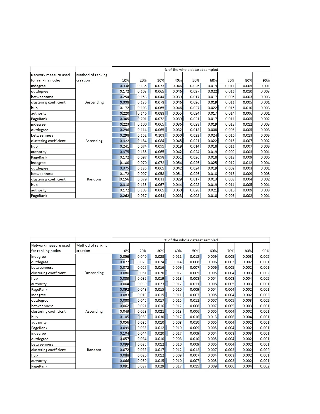
1 Learning in Unlabeled Networks — An Acti v e Learning and Inference Approach T omasz Kajdano wicz 1 , Radosław Michalski 1 , Katarzyna Musial 2 , Przemysław Kazienk o 1 1 Wr ocław University of T echnology Department of Computational Intelligence Wr ocław , P oland E-mail: tomasz.kajdanowicz@pwr .edu.pl, radoslaw .michalski@pwr .edu.pl, kazienko@pwr .edu.pl - 2 Bournemouth University F aculty of Science and T echnology Bournemouth, UK E-mail: kmusialgabrys@bournemouth.ac.uk The task of determining labels of all netw ork nodes based on the knowledge about netw ork structure and labels of some training subset of nodes is called the within–network classi- fication. It may happen that none of the labels of the nodes is known and additionally there is no information about num- ber of classes (types of labels) to which nodes can be as- signed. In such a case a subset of nodes has to be selected for initial label acquisition. The question that arises is: ”la- bels of which nodes should be collected and used for learn- ing in order to provide the best classification accuracy for the whole network?”. Acti ve learning and inference is a practical framew ork to study this problem. In this paper , set of methods for activ e learning and infer- ence for within network classification is proposed and vali- dated. The utility score calculation for each node based on network structure is the first step in the entire process. The scores enable to rank the nodes. Based on the created rank- ing, a set of nodes, for which the labels are acquired, is se- lected (e.g. by taking top or bottom N from the ranking). The new measure–neighbour methods proposed in the paper sug- gest not obtaining labels of nodes from the ranking but rather acquiring labels of their neighbours. The paper examines 29 distinct formulations of utility score and selection methods reporting their impact on the results of two collectiv e classi- fication algorithms: Iterativ e Classification Algorithm (ICA) and Loopy Belief Propagation (LBP). W e advocate that the accuracy of presented methods de- pends on the structural properties of the examined network. W e claim that measure–neighbour methods will work bet- ter than the regular methods for networks with higher clus- tering coefficient and worse than regular methods for net- works with lo w clustering coefficient. According to our hy- pothesis, based on clustering coefficient of a network we are able to recommend appropriate acti ve learning and inference method. Experimental studies were carried out on six real–world networks. In order to in vestigate our hypothesis, all analysed networks were categorized based on their structural charac- teristics into three groups. In addition, the representativ eness of initial set of nodes for which the labels are obtained and its influence on classification accuracy was e xamined. Ke ywords: complex networks, network analysis, classifica- tion, classification in networks, within network classification, activ e learning, selection of starting nodes for classification, ICA, LBP . 1. Introduction In many real–world networks, a set of nodes and connections between them are known b ut the informa- tion about their characteristics can be fragmentary and not coherent. On many occasions, howe ver , the infor- mation about nodes’ labels is essential, e.g. knowing users’ preferences or demographic profile is needed in the process of personalised recommendation of prod- ucts or services. Of course, all labels can be obtained by asking ev erybody about them but, due to the scale of some networks and anonymity of many users in the online world, it may be a very time–consuming, costly and ineffecti ve process. In order to reduce the resources required for manual acquisition of labels for all nodes, more sophisticated method, which enables to uncover labels of only limited number of nodes and based on this knowledge to perform the automatic clas- sification for the rest of nodes, is needed. The research presented in this paper aims at addressing this issue by proposing an effecti ve method for selection of starting nodes and acquisition of their labels that will serve as a training set for within network classification task. W e also claim that there is no method that will work accurately in all cases and we sho w in our experiments Preprint, this article has been accepted to AI Communications V ol. 29, No. 1, 2016, IOS Press 2 that the accurac y of dif ferent methods strongly depend on some of the structural characteristics of a network. For the illustration purposes we present an exam- ple of marketing campaign that will help to under- stand presented research. Let us assume that a market- ing campaign has to be addressed to a giv en commu- nity of customers. The knowledge about relationships between customers is a v ailable (e.g. derived from their monitored interactions), hence, we can create a cus- tomer social network. The main purpose of the cam- paign is to propose new product only to those who are likely to buy it within the next year . Howe ver , the top management allocates to the campaign only a fixed amount of resources, which is not sufficient to target all community members. Thus, the question is which customers should be initially targeted in order to opti- mise the return on in vestment (R OI) of the entire cam- paign. R OI strongly depends on the quality of classi- fication of community members into two classes: (i) customers and (ii) non–customers as we sav e resources by not sending the offer to non–customers. One of the approaches to model the campaign is to use collective classification. In order to perform collec- tiv e classification task, it is required to retrie ve class la- bels for an initial population of nodes and next to use it in the inference process. Before classifying the whole network, some selected nodes need to be pro vided with the offer and their positive and negati ve responses to- gether with the response rate should be collected. Af- terwards, based on theirs behaviour as well as relation- ships between social network nodes, collective classifi- cation could model responses for the remaining nodes. The main issue is to determine which nodes should be selected to acquire their labels in order to maximise the performance of classification. An intuitive answer is that we should start with the nodes estimating the whole network most accurately . The solutions of the problem of which nodes’ labels should be obtained in order to perform the collectiv e classification are called active learning or active infer ence appr oaches because they activ ely , not randomly , support selection of the learning set. The problem of selecting appropriate nodes in or- der to start collectiv e classification process is studied in this paper . First, the literature re view in the areas of (i) collective classification, as well as (ii) activ e learn- ing and inference methods is described in Section 2. Section 3 presents the method for selection of initial nodes for classification purposes proposed in this paper and in Section 4 there are rev oked basic collective clas- sification algorithms. The experiments using the pro- posed method and the datasets used in the process are described in Section 5 and discussed in Section 6. Fi- nally , Section 7 summarises the main contribution of the paper . 2. Related work The research area that is in the focus of this paper is activ e learning and inference methods for within net- work classification and the literature that relates to this topic is presented belo w . Howe ver , first the problem of collectiv e classification is discussed to give a general background of the field and facilitate the understanding for non–expert readers. 2.1. Collective classification Although problem of classification in traditional ma- chine learning is not new , together with the explosion of W eb–based social networks [23], the new branch in this area called collective (relational) classification has emerged. The main difference between collectiv e classification and traditional approach to classification problem is that the former one allows data to be de- pendent whereas the latter one assumes independent and identically distributed data (i.i.d.). Collectiv e ap- proach allo ws to consider both characteristics of nodes and topology of the network in the process of assign- ing node to a specific class. It means, that not only features of a node to be classified are taken into ac- count b ut also the attributes and labels of related nodes (e.g. direct neighbours) can be considered [16]. T wo approaches can be distinguished for classification of nodes in the network (i) within-network (Figure 1) and (ii) across-network inference (Figure 2). In the within- network classification [10] training nodes are directly connected to nodes whose labels are to be assigned in the classification process. In the across-network clas- sification [22] models learnt from one network are ap- plied to another similar network. One of the issues in collectiv e classification is to de- termine set of features that should be used in order to maximize the classification accuracy . Recent research in this area shows that the v alues of ne w attributes de- riv ed from structural properties of the graph, such as betweenness centrality , may improve the accuracy of the classification task [14]. Another confirmation of that fact and some more discussion about it comes from other research [18]. Another element that should be considered in the collectiv e classification is the order 3 Fig. 1. An illustration of within-network classification task. Fig. 2. An illustration of across-network classification task. of visiting nodes in the graph to perform re–labelling. The order of visiting the nodes influences the values of input values deriv ed from the structure. T o address that problem variety algorithms hav e been proposed. Random ordering [20] is a simple strategy used with iterativ e classification algorithms and can be quite ro- bust. Another and most popular e xamples of collecti ve classification methods are: Iterativ e Classification Al- gorithm (ICA) and Gibbs Sampling Algorithm (GSA), introduced by Geman & Geman in the image process- ing conte xt [15]. Both of them belong to so called ap- proximate local inference algorithms that are based on local conditional classifiers [30]. Next technique is a Loopy Belief Propagation (LBP) [28] that is a global approximate inference method used for collectiv e clas- sification. But, according to recent studies [17], abov e mentioned methods are not robust enough to work ef- ficiently and accurately in sparsely labelled and large- scale environments. This is a very important conclu- sion as majority of W eb– and technology–based social networks are very sparse and large. Another drawback is that the y cannot be easily deployed within multi- dimensional networks [19], what creates space for de- veloping ne w , robust collecti ve classifiers. According to [12], a very promising area of re- search, which may contrib ute to solve the issues iden- tified above, is b uilding compound ensemble collective classifiers. As it has been already sho wn, despite the fact that ensemble methods are performing accurately for i.i.d. data, there is a lack of similar analysis for re- lational data. For instance, in [7] it was presented that bagging reduces total classification error in i.i.d. data by reducing the error due to variance. The extension of i.i.d. ensembles to improve classification accuracy for relational domains has been shown in [11]. That in- cludes a method for constructing ensembles while ac- counting for the increased variance of network data and an ensemble method for reducing variance in the in- ference process. Another promising work [13] sho wed that dif ferent ensemble method – stacking – improves collectiv e classification by reducing inference bias. 2.2. Active learning and infer ence in networks As mentioned abov e activ e learning and inference are methods used to select nodes for which labels should be acquired in order to perform collecti ve clas- sification [1], [31], [32], [2], [29]. The main goal of these methods is to impro ve classification accuracy by choosing nodes in a non-random way . In contrast to passiv e methods where all labels are obtained once, ac- tiv e methods perform this task iterati vely . Research re- sults sho w , that in order to achie ve similar accuracy , in some cases number of nodes to be queried for labels is logarithmic when comparing to passi ve methods [4]. It should also be emphasized that the goal of acti ve infer - ence and learning methods is different than e.g. seed- ing strategies where the most influential nodes are se- lected. Acti ve inference and learning in the context of collectiv e classification aims at selecting nodes that en- able to minimize the classification error for the whole network. The main drawback of acti ve learning and in- ference methods is that the set of queried labels is los- ing its i.i.d. characteristics, what may lead to spending querying b udget on bias sampling [34] or propagating the information in areas, where surrounding nodes may cov er the inner ”islands” that are labeled differently [5]. T o overcome some of the discussed limitations ac- tiv e inference and learning offer different approaches when dealing with separable and non-separable data, e.g. agnostic activ e learning [3] or query by committee [33]. One of the approaches to activ e learning in relational data is Reflect and Correct (RA C) method introduced in [5] and further dev eloped in [6]. It is based on a sim- ple intuition that the misclassified nodes are gathered close to each other; they are clustered together . Thus, misclassifying one node might cause wrong labelling of neighbours. Therefore, it is reasonable to acquire the actual label of representativ e nodes from such clusters 4 and use it in the inference. In order to find these clus- ters a label utility function can be applied [6]. Authors introduce three types of features – local, relational and global – which are used as a learner of the classifier . These features measure three dif ferent aspects of mis- classification. Local feature focuses on the attrib utes of a node, the relational takes into consideration its neigh- bourhood and the global feature measures the differ - ence between the prior belief about the class distribu- tions and posterior distributions based on the predic- tions. Having all these features av ailable, authors of [6] use a training graph and the predictions of a collective model on this graph to learn the distrib ution of labels. This approach presents a reasonable assumption that we are having some budget to spend for acquiring la- bels. Authors compared the results of the introduced RA C method against two other approaches including their viral marketing approach and greedy acquisition showing that RA C method outperforms the others. Another approach was proposed in [25]. The paper introduces a technique for node selection in an active learning framew ork. It selects a set of nodes that should be used in the collecti ve classification based on a given limited budget. Using the idea of smoothness (similar distributions of independent attributes as well as rela- tional features between nodes) it decides which nodes to select. The smoothness idea incorporates high util- ity from nodes that are close to each of the queried nodes. It is also proposed how to compute utility for each non–surv eyed node and how to sample within the budget. Howe ver , in this method, authors assumed that network structure may not be av ailable a priori, so the queries may reflect the labels and the neighbourhood of the node. A similar approach has been introduced in relational acti ve learning proposal in [21]. The key idea behind this approach was to select these nodes to acquire the label, whose predictions are potentially most certain. It is w orth to emphasize that this is incon- sistent with many con ventional utility metrics used in i.i.d. settings, which fav our labelling nodes with high uncertainty . 3. Relational active lear ning and infer ence 3.1. The method for active learning and infer ence in within–network classification based on node selection The proposed method for active learning and infer- ence in within-network classification task consists of fiv e main steps, see Figure 3. First, for a gi ven un- labelled network, the utility scores for each network node are obtained by calculating the node’ s structural measures such as degree centrality , closeness central- ity , etc. In general, the utility score should reflect the usefulness of the node’ s label in the process of within– network classification. Further discussion on consid- ered utility scores is provided in Section 3.2. In addi- tion, new ’measure’–neighbour approaches for assess- ment of the nodes’ utility have been proposed in Sec- tion 3.3. Afterwards, the previously obtained utility scores are sorted in the ascending or descending order; it en- ables to form nodes’ ranking. Depending on the type of the utility score, the most useful nodes are these with the highest or smallest score value. In the next step, the method selects nodes for which the label will be queried based on top N items in the ranking. Once the process of label acquisition is completed, the ap- propriate relational classification algorithm can be ap- plied to perform within–network classification. Note, that this last step is not the main contribution of the paper and man y different classification algorithms can be applied. In this research two of them were selected as the most representative and widely used, i.e. Itera- tiv e Classification Algorithm (ICA) and Loopy Belief Propagation (LBP). 3.2. Utility scor es Utility scores reflect the usefulness of the node’ s la- bel in the process of within–network classification. It is expected that learning the relational classification model using some previously acquired labels will re- sult with small classification error . The process of label acquisition in activ e learning should be expressed as simple optimization problem of nodes selection, b ut in the within–network classification setting it is not pos- sible. The general requirement of the selection mech- anism is to pick those nodes’ labels from label set L whose usage in relational inference will result in the smallest possible misclassification error E . In general terms, the expected misclassification er- ror for all unlabelled nodes v i ∈ V U K on their labels Y U K i with x i attributes depends on abilities of relational classification algorithm Φ that is learnt on previously acquired labels Y K for the initial node set: ∑ Y i \ Y K E ( Y i | X = x i , Y K , Φ ( Y K )) (1) 5 Fig. 3. Major steps of the activ e learning and inference method for within-network classification. Therefore, the main problem is to obtain unkno wn val- ues of Y K for which classification algorithm Φ will provide proper results. Then, the aggregated error must reflect an expectation o ver all possible v alues of Y K : ∑ Y i \ Y K ∑ l ∈ L P ( Y K = l ) E ( Y i | X = x i , Y K = l , Φ ( Y K = l )) (2) where P ( Y K = l ) is the chance that Y K takes a value of label l . Although the presented error is in general suitable for across–network classification, it does not comply with within–network classification. It is im- possible to assess the correctness of classification for all nodes related to Y i \ Y K due to the lack of these la- bels. Thus, it is impossible to propose an y utility score that will directly lead to classification error minimiza- tion. Nev ertheless, it is still possible to make use of other utility scores that reflect structural properties of nodes, relying on the assumption that classification error de- pends on these measures. Depending on the charac- teristics of the underlying network, a proper measure can be chosen from the v ast variety of nodes structural measures [24] such as indegree centrality , outdegree centrality , betweeness centrality , clustering coeficient, hubnes, authority , page rank. 3.3. A new ’measur e’–neighbour appr oach to utility scor e T o extend the typical structural measures approach, enumerated in Section 3.2, authors proposed and ev al- uated another method. Assuming that some nodes with the highest measures’ values may actually be located on the border of ’classes’, it may be useful to pick not this node itself, but its neighbours. The intuition suggests that it may hold especially for the between- ness or page rank measures, since nodes with high be- tweenness and page rank may be located at the bor- der of clusters or groups or may ev en play the role of bridges. In this case, it may be worth acquiring the la- bel of the neighbour instead of the bridge label itself. For example, in the case of betweenness, we identify nodes with the highest value of betweenness and se- lect their neighbours for label acquisition. By analogy , we can create indegree–neighbour utility score, page rank–neighbour utility score, etc. All of them focus on neighbours of nodes with a giv en property . In order to confirm or reject the above concept, the authors performed set of experiments comparing the results of this approach with the typical measure–based methods, see e.g. T able 4 and 6. The neighbour selection heavily depends on the structure of the network. It may happen that in partic- ular cases some nodes selected from rankings do not hav e neighbours. Therefore actual number of neigh- bouring nodes may be smaller than the size of sampled ranking. It was assumed that for each selected node from ranking it is selected only one neighbour . Thus, for instance if it is selected 10% of nodes from the network according to particular ranking, we may end up with smaller than 10% population of network con- stituted by neighbours (see Figure 13). Moreover , for the propagation algorithm (LBP) when a node from the training set has no neighbours, the information about the label during the classification process will not be propagated. On the contrary the ICA method does not depend on network structure in the sense that even if the labelled node has no neighbours, the label may be assigned to nodes in other, e ven disconnected, compo- nents. 6 Howe ver , in general, this did not have adverse ef fect on the obtained results. The exception was one dataset (CS PHD) where the netw ork was highly disconnected and almost no nodes were labelled in the neighbour al- gorithm. In other cases, despite the f act that less nodes were used as an input to classification algorithm, LBP– neighbour method outperformed classical LBP in both approaches – top and bottom (i.e. when initial nodes were selected from top and bottom of the rankings cre- ated based on the utility scores respectiv ely). 4. Within-netw ork classification algorithms There exist several algorithms for within-network classification. T wo of them were utilized in experi- ments in Section 5. The first algorithm is the Iterati ve Classification Al- gorithm (ICA). The basic idea behind ICA is quite sim- ple. Considering a node v i ∈ V U K , where V U K is a set of nodes with unknown labels, V U K ⊂ V and V is the set of all nodes in the network, we aim at discover - ing v i ’ s label l i . Having labels of v i ’ s neighbourhood known, ICA utilizes a local classifier Φ that takes the attribute values of nodes with known labels ( V K ) and returns the most appropriate label value l i for v i from the class label set L , i.e. l i ∈ L . If the knowledge of the neighbouring labels is only partial, the classifica- tion process needs to be repeated iterati vely . In each it- eration, labelling of each node v i is done using current best estimates of local classifier Φ and continues until the label assignments stabilize. A local classifier might be an y function that is able to accomplish the classifi- cation task. It can range from simple to complex mod- els like Nai ve Bayes, decision tree or SVM. Algorithm 1 depicts the ICA algorithm as a pseudo- code where the local classifier is trained using the initially labelled nodes V K . It can be observed that the attributes utilized in classification depend on the current label assignment (lines 8 and 9 in Algorithm 1). Thus, the repetition of classification phase needs to be performed until labels stabilize or the maxi- mum number of iteration is reached. Computation of nodes’ attrib utes (line 2 and 8) is the calculation of various nodes’ structural measures describing profile of each no de, including label–dependent and/or label– independent features [18]. Note that optimization of the model (line 4) is based on the local knowledge, since x i attribute of v i reflects only local information with v i ’ s perspectiv e. Algorithm 1 Iterativ e Classification Algorithm (ICA), the idea based on [30] 1: for each node v i ∈ V U K do 2: compute x i , i.e. v i ’ s attributes using the observed (known) nodes from V K 3: end for 4: train classifier Φ by Θ optimization using the at- tributes of V K nodes 5: repeat 6: generate ordering O ov er nodes in V U K 7: for each node v i ∈ O do 8: compute x i , i.e. v i ’ s attributes using current assignments 9: l i ← Φ ( x i , Θ ) 10: end for 11: until label stabilization or the maximum number of iterations is reached Another method applied in experiments was the Loopy Belief Propagation algorithm (LBP). It is an al- ternativ e to ICA approach to perform collectiv e classi- fication. The main difference is that it defines a global objectiv e function to be optimized, instead of perform- ing local classifier optimization (ICA). LBP is an iterativ e message–passing algorithm. The messages are transferred between all connected nodes v i and v j ; where v i , v j ∈ V , ( v i , v j ) ∈ E , E is the set of network edges. These messages might be interpreted as belief to what extent v j label should be based on v i label. The global objective function, which is optimized in LBP , is deriv ed from the idea of pairwise Markov Ran- dom Field (pairwise MRF) [35]. In order to calculate the message for propagation, the calculation presented in Eq. 3 is performed. m i → j ( l j ) = α ∑ l i ∈ L Ψ i j ( l i , l j ) φ ( l i ) ∏ v k ∈ V U K \ v j m k → i ( l i ) (3) where m i → j ( l j ) denotes a message to be sent from node v i to v j , α is the normalization constant that ensures each message to sum to 1, Ψ and φ denote the clique potentials. For further details please see [30]. The calculation of believ e b ( l i ) for node v i can be expressed as in Eq. 4: b ( l i ) = αφ ( l i ) ∏ v j ∈ V U K m j → i ( l i ) (4) The LBP algorithm consists of two main phases: message passing that is repeated until the messages are stabilized and believ e computation, see Algorithm 2. 7 Algorithm 2 Loopy Belief Propagation (LBP), the idea based on [30] 1: for each edge ( v i , v j ) ∈ E , v i , v j ∈ V U K do 2: for each class label l i ∈ L do 3: m i → j ( l ) ← 1 4: end for 5: end for 6: //perform message passing 7: repeat 8: for each edge ( v i , v j ) ∈ E , v i , v j ∈ V U K do 9: for each class label l i ∈ L do 10: m i → j ( l j ) ← α ∑ l i ∈ L Ψ i j ( l i , l j ) φ ( l i ) 11: ∏ v k ∈ V U K \ v j m k → i ( l i ) 12: end f or 13: end for 14: until stop condition 15: //compute beliefs 16: for all v i ∈ V U K do 17: for all l i ∈ L do 18: b i ( l i ) ← αφ ( l i ) ∏ v j ∈ V U K m j → i ( l i ) 19: end for 20: end for 5. Experiments 5.1. Experimental set–up In order to e v aluate the proposed method for ac- tiv e learning and inference in terms of classification accuracy , the Iterativ e Classification (ICA) and Loopy Belief Propagation (LBP) algorithms were tested with various utility scores. The e xperimental scenario aims at e xamining the follo wing structural measures used as utility scores: – indegree centrality , – outdegree centrality , – betweenness centrality , – clustering coefficient, – hubness, – authority , – page rank. All of them were applied in two selection methods: nodes with the top (the greatest) and bottom (the small- est) values of indi vidual scores. Independently , another new ’measure’–neighbour method proposed in Section 3.3 was also ev aluated. Its idea is to chose the neigh- bours of the node with the greatest/smallest value of a giv en utility score. In total, 29 selection methods were tested: 14 for original structural measures (7 measures; ’top’ or ’bot- tom’ for each), 14 for ’measure’–neighbour methods and a random selection. The random selection was re- peated 14 times and the average error was taken as its final validation result. The experiments were carried out on original dataset with labels acquired according to particular setting of selection method and utility score. Thanks to that, each dataset was split into known and unknown node sets. The models were learnt on acquired labels in nine dis- tinct proportions (from 10% to 90% of known labels) and tested on the remaining part. In order to ev alu- ate the quality of classification, the classification error was recorded. According to pre viously gathered expe- rience on the configuration of the classification algo- rithms [17] the implementation of ICA was based on Random Forest base classifier [8] and it we used 50 it- erations or 0 . 01 as relati ve change of labels in the LBP as the stop condition. ’Measure’–neighbour v ersion of training set selection (Section 3.3) used a draw with the uniform distribution from adjacent nodes. 5.2. Datasets The experiments were carried out on six datasets. The AMD NETWORK graph presents attendance at the conference seminars. The dataset was a result of the project that took place during ”The Last HOPE” Conference held in July 18-20, 2008 in New Y ork City , USA. The Radio Frequency Identification devices were distrib uted among participants of the conference that allowed to identify them uniquely and to track what sessions they attended. The dataset was built from the information about descriptions of participants’ in- terests, their interactions via instant messages, as well as their location ov er the course of the conference. Lo- cation tracking allowed to extract a list of attendances for each conference talk. In general, the most interest- ing data from the experiment point of vie w are: infor- mation about conference participants, conference talks and presence on the talks. Another genealogy dataset CS PHD is the network that contains ties between PhD students and their ad- visors in theoretical computer science field where the arcs lead from advisors to students [27]. The third dataset NET SCIENCE contains a co- authorship network of scientists working in the area of network science [26]. It was extracted from the bibli- ographies of two re vie w articles on networks. Another biological dataset YEAST is a protein- protein interaction network [9]. 8 The P AIRS FSG dataset is a dictionary from the Univ ersity of South Florida with word association, rhyme and word fragment norms. Its graph reflects cor- relations between nouns, verbs and adjectiv es. In the experiments we use the original P AIRS FSG data as well as its reduced version P AIRS FSG SMALL. The profiles of all datasets were shortly depicted in T able 1. In order to in vestigate our hypothesis that the accuracy of classification depends on network charac- teristics, the datasets were divided into three groups (see column ’Group’ in T able 1 as well as description of groups in T able 2). It was done based on the com- monly used network’ s characteristics, such as average node degree, a verage path length, modularity , graph density , network diameter, and average clustering co- efficient of nodes. Based on those characteristics, net- works that belong to Group 1 are small–world net- works, those that belong to Group 2 are non–small– world modular networks and those in Group 3 are ran- dom networks that are very sparse (at the edge of phase transition condition for random networks). The graphs that belong to the first group have short av erage path length, the smallest network diameter out of all analysed networks, and clustering coefficient larger than 0.3. W ith relati vely large clustering coeffi- cient and short average path length networks in group 1 exhibit characteristics of small–world netw orks. The second group contains networks with moderate aver - age path length, modularity from the range ( 0 . 5; 0 . 9 ) , graph density from the range ( 0 . 01; 0 . 1 ) and clus- tering coefficient smaller than 0 . 15. Those character- istics indicate that networks in this group are non– small–world modular netw orks. Group 3 contains only one dataset which is highly disconnected, with many isolated nodes, density and clustering coef ficient ap- proaching zero, and over 400 nodes with node degree equal to 0. This group represents random networks with very low probability that the link will exist be- tween two randomly selected nodes, which means that the giant component is not present and such networks consist of many small connected components. Further detailed characteristics of the networks followed by in- formation about number of distinct classes are av ail- able in the Supplement Material in Sections 1 and 2. 6. Experimental results and discussion As the experiments were performed using large number of parameters, the obtained results can be anal- ysed from man y dif ferent perspecti ves. Overall, it can be noticed that accuracy of the in vestigated approaches varies and the methods themselves cannot be compared in a straightforward way . This is clearly visible in Fig- ure 4 depicting results obtained for the best combina- tion of ICA, ICA neighbour , LBP , and LBP neighbour settings and compared with random selection. All of the results are presented in T ables 3, 4, 5 and 6. There are three basic factors that influence the out- put. The first one is the structural profile of the net- work, the second is the method of selecting nodes for the initial label acquisition (seed selection strategy), and the third one is the method of within–network col- lectiv e classification. Also, the percentage of uncov- ered classes during the initial selection process con- tributes to the classification accurac y . In general, there is no single node selection method combined with inference concepts that would be best for e very kind of network and ev ery size of initial node set. Howe ver , some approaches and combinations of the reasoning algorithms with seed acquisition meth- ods are better than others for particular network pro- files, see Section 6.1. This would suggest that the re- sults depends on the network profile. One of the observations that can be deriv ed from the experimental results is the better performance of node selection methods based on ’measure’–neighbour approach described in Section 3.3 compared with the original rankings, especially for datasets in groups 1 and 2. This suggests that the bigger the clustering co- efficient of the network, i.e. the higher probability that the clusters will exist in the network, the better the clas- sification results. It is visible, if we juxtapose results for individual measures from T able 3 with T able 4 and from T able 5 with T able 6. The comparison showing how often top or bottom of ranks for given measures outperformed each other is presented in T able 7. As a result, ’measure’–neighbour methods more often sur- pass random selection than the measure based meth- ods, see the last column in T able 4 and 6. Moreover , while analysing the last column in T ables 3, 4, 5, and 6, we can find out that there is alw ays at least one ICA and at least one LBP node selection method outper- forming the random approach. In some cases, e.g. for AMD and P AIRS FSG (T ables 4 and 6), all or almost all ’measure’–neighbour methods are better than ran- dom selection. The proof for existence of some meth- ods better than random in any case is very important from practical point of view . It justifies that searching for more ef fectiv e inference methods can always be successful. Experimental results also revealed that, regardless of the kind of nodes’ selection method in acti ve learning 9 (a) AMD dataset (group 1) (b) NET SCIENCE dataset (group 1) (c) P AIRS FSG dataset (group 2) (d) P AIRS FSG SMALL dataset (group 2) (e) YEAST dataset (group 2) (f) CS PHD dataset (group 3) Fig. 4. Comparison of classification error for ICA and LBP; both only for their most efficient utility scores for original utility scores and ’measure’-neighbour variants. 10 (degree, betweenness, etc.) and selection strate gy (top or bottom of the ranking), none of the methods was able to satisfactory generalize networks that are very sparse and random by nature (especially for network CS PHD which belongs to group 3, see Section 5.2). For such problem, the results were quite similar to ran- dom seeding, see T ables 3, 4, 5 and 6. When analysing the activ e learning method giving the best results for ICA, in most cases, the inference results were not as much susceptible to the percent- age of known nodes as for the LBP method. It means that the global network propag ation of information ap- plied by LBP is more dependent on the size of the training set than ICA method. In general, acquisition of labels by means of the best proposed methods (e.g. nodes with the greatest degree or neighbours of nodes with the lowest page rank) in conjunction with ICA and LBP algorithms, in most cases, outperformed random results. Howe ver , when using LBP the results might suffer from its basic property: if the selection method does not provide nodes from all connected components then the information about labels is not propagated to separated parts of the network. In addition, as it was described in Section 4, the Loopy Belief Propagation (LBP) method is heavily network dependent, because the underlying network structure and global objective function determine the propagation, while the ICA method utilizes only the local structure of the network. The experimental re- sults confirm that these dif ferences hea vily influenced the results of indi vidual classification methods. F or ex- ample compare results for AMD and NET SCIENCE (good performance of LBP for small–world like net- works) with CS PHD (the poor LBP results for the loosely connected network with small node degree). 6.1. Influence of network char acteristics on classification r esults T o facilitate the analysis of the large number of ex- perimental results, for each group of networks pre- sented in Section 5.2, the appropriate ’ results pro- file’ has been created (see T able 2). Classification per - formed on the networks from group 1, which can be characterised as networks that exhibit small–world phenomenon, features good accuracy of ’measure’– neighbour methods with LBP neighbourhood (bottom page rank) outperforming other approaches. In addi- tion, most of the ’measure’–neighbour methods out- perform random case. Classification error, which for this group is high for small training sets, substantially decreases for the bigger training sets. Classification results for the second group of networks exhibit rel- ativ ely small variance of error . In general, the more classes in the dataset, the worse classification accu- racy . Moreover , for smaller modularity and density as well as greater clustering coefficient LBP neighbour approach outperforms others. Finally , for the third group of networks, which are close to random networks with a very low connecti vity probability , ’measure’–neighbour methods are worse than original and random approaches. The classifica- tion results are rather poor for all cases, b ut due to the fact that ICA method does not depend on connections within network for classification, it outperforms LBP- based methods. Additionally , we performed a set of robust fit re gres- sions in order to in vestigate the relation between struc- tural properties and the results of the classifications (see Figures 5, 6, 7, and 8). For this part of the study by results we understand the number of times when a giv en approach (ICA measure based, ICA measure- neighbour based, LBP measure based, LBP measure- neighbour based) was better than random for each analysed network (sum of the last column from T a- bles 3, 4, 5, 6 for each network). W e took into account two metrics: (i) clustering coefficient and (ii) av erage path length as those are the measures that enable to classify networks as random, small–world or ordered ones. Results sho w that for measure–based methods (for both ICA and LBP approaches) the smaller the clustering coefficient and the bigger the average path length the better the performance of the classifica- tion. Exactly opposite trend is visible for measure- neighbour approaches. Howe ver , we should rather ne- glect the results for a verage path length as in all cases R 2 is very close to 0. Concentrating on clustering co- efficient metric and the obtained results we can make a recommendation that for networks that are discon- nected and very random in their nature (Group 3) we should use measure–based selection strategies and for networks that are connected (Group 1 and 2) we should rather apply ’measure’–neighbour selection strategies. 11 T able 1 Basic properties of datasets utilized in experiments. Dataset Group Nodes Edges Directed Classes (la- bels) A vg. node degree A vg. path length No. of connected compo- nents Modularity Graph density Network Diameter A vg. nodes clustering coeff. AMD NETWORK 1 319 34385 no 16 215.58 1.322 1 0.102 0.678 2 0.824 NET SCIENCE 1 1588 2742 yes 26 1.727 1.997 395 0.955 0.001 7 0.319 P AIRS FSG 2 4931 61449 yes 3 12.462 4.278 1 0.594 0.003 10 0.122 P AIRS FSG SMALL 2 1972 12213 yes 3 6.193 5.358 13 0.688 0.003 14 0.127 YEAST 2 2361 7182 yes 13 3.042 4.648 59 0.59 0.001 16 0.065 CS PHD 3 1451 924 yes 16 0.636 2.265 531 0.967 0 10 0.001 T able 2 The description of groups of datasets and profiles of their collectiv e classification results. Group Datasets Network profile Results profile 1 AMD NETWORK, NET SCIENCE small–world profile-like, short avg. path length; the smallest network diameter; clus- tering coeff. > 0.3 high error level decreasing with for increasing % of training set; good performance of ’measure’-neighbour methods; LBP neighbour (bottom page rank) outperforms the others; most of ’measure’-neighbour methods outperform random 2 YEAST , P AIRS FSG, P AIRS FSG SMALL non–small–world modular networks, moder- ate a vg. path length; modularity ∈ ( 0 . 5; 0 . 9 ) ; graph density ∈ ( 0 . 01; 0 . 1 ) ; clustering coeff. < 0.15 relativ ely small v ariance of results; the more classes, the worst results; for smaller modularity and density , and greater cluster- ing coeff. LBP-neighbour outperforms the others 3 CS PHD random–like network with very low proba- bility of edges between nodes, highly discon- nected; many isolated nodes (avg. node de- gree < 0.7); density 0; clustering coef f. close to 0 LBP error > 0.8; ICA better than LBP , but still poor; ’measure’-neighbour methods w orse than original and random 12 T able 3 Classification error in active learning based on ICA for distinct selection strategy; initial nodes taken directly from the ranking. Note: the last column represents how man y of the non–random selection strategies outperformed the random case. Dataset Lab. nodes T op inde- gree T op out- de- gree T op be- twee- ness T op clust. coeff. T op hub- ness T op au- thor- ity T op page rank Down inde- gree Down out- de- gree Down be- twee- ness Down clust. coeff. Down hub- ness Down au- thor- ity Down page rank Random # bet- ter 10% 0.983 0.983 0.91 0.879 0.976 0.976 0.91 0.875 0.875 0.896 0.91 0.875 0.875 0.875 0.906 7 20% 0.883 0.883 0.902 0.981 0.883 0.883 0.883 0.898 0.898 0.906 0.898 0.938 0.938 0.898 0.878 0 30% 0.897 0.897 0.906 0.875 0.911 0.911 0.933 0.884 0.884 0.853 0.897 0.911 0.911 0.884 0.858 1 40% 0.943 0.943 0.906 0.938 0.885 0.891 0.885 0.912 0.912 0.927 0.943 0.912 0.912 0.917 0.837 0 AMD 50% 0.881 0.881 0.888 0.919 0.881 0.969 0.931 0.95 0.95 0.9 0.906 0.95 0.95 0.95 0.831 0 60% 0.961 0.961 0.914 0.906 0.875 0.875 0.961 0.914 0.914 0.914 0.898 0.891 0.891 0.891 0.811 0 70% 0.969 0.969 0.906 0.938 0.948 0.948 0.906 0.833 0.833 0.948 0.896 0.833 0.958 0.833 0.798 0 80% 0.938 0.938 0.922 0.969 0.953 0.953 0.938 0.938 0.938 0.969 0.953 0.938 0.938 0.938 0.805 0 90% 0.938 0.938 0.938 0.875 0.906 0.906 0.938 0.938 0.938 0.875 0.906 0.906 0.906 0.938 0.782 0 10% 0.967 0.969 0.941 0.944 0.954 0.935 0.934 0.973 0.91 0.922 0.919 0.936 0.935 0.94 0.935 4 20% 0.935 0.925 0.933 0.926 0.916 0.918 0.92 0.911 0.909 0.922 0.914 0.942 0.915 0.923 0.911 2 30% 0.906 0.904 0.933 0.902 0.902 0.922 0.912 0.914 0.911 0.915 0.921 0.925 0.918 0.916 0.908 4 40% 0.932 0.909 0.923 0.911 0.903 0.91 0.915 0.93 0.909 0.912 0.923 0.903 0.925 0.92 0.902 0 NET SCIENCE 50% 0.914 0.904 0.912 0.899 0.915 0.918 0.922 0.91 0.899 0.922 0.91 0.926 0.914 0.912 0.899 2 60% 0.906 0.911 0.925 0.901 0.923 0.913 0.923 0.925 0.954 0.911 0.916 0.923 0.927 0.904 0.898 0 70% 0.916 0.916 0.92 0.902 0.911 0.916 0.923 0.925 0.923 0.913 0.907 0.902 0.907 0.913 0.898 0 80% 0.891 0.908 0.922 0.911 0.922 0.911 0.922 0.922 0.98 0.932 0.918 0.898 0.915 0.928 0.898 2 90% 0.884 0.898 0.898 0.905 0.932 0.918 0.925 0.905 0.925 0.939 0.905 0.918 0.918 0.905 0.896 1 10% 0.855 0.984 0.845 0.845 0.761 0.887 0.839 0.815 0.807 0.85 0.85 0.882 0.85 0.815 0.824 4 20% 0.816 0.889 0.88 0.949 0.855 0.913 0.834 0.883 0.837 0.84 0.955 0.946 0.955 0.56 0.777 1 30% 0.928 0.938 0.959 0.993 0.828 1 0.841 0.607 0.945 0.89 0.993 0.938 0.976 0.607 0.66 2 40% 0.892 0.864 0.988 0.92 0.912 0.948 0.9 0.61 0.936 0.679 0.928 0.888 0.908 0.61 0.643 2 P AIRS FSG 50% 0.291 0.295 0.302 0.335 0.32 0.29 0.349 0.329 0.319 0.337 0.292 0.333 0.339 0.334 0.308 5 60% 0.288 0.295 0.295 0.335 0.325 0.284 0.293 0.328 0.325 0.331 0.28 0.312 0.443 0.528 0.307 6 70% 0.279 0.297 0.293 0.332 0.33 0.28 0.291 0.335 0.313 0.341 0.279 0.313 0.528 0.346 0.306 6 80% 0.27 0.293 0.259 0.333 0.339 0.271 0.276 0.344 0.308 0.35 0.26 0.297 0.439 0.36 0.309 8 90% 0.257 0.296 0.237 0.326 0.342 0.263 0.263 0.362 0.3 0.37 0.281 0.281 0.577 0.383 0.305 8 10% 0.671 0.668 0.683 0.668 0.689 0.695 0.687 0.661 0.669 0.701 0.704 0.709 0.7 0.699 0.665 1 20% 0.654 0.678 0.695 0.695 0.715 0.715 0.697 0.671 0.657 0.713 0.737 0.732 0.734 0.706 0.661 2 30% 0.668 0.673 0.715 0.709 0.735 0.736 0.701 0.68 0.669 0.738 0.739 0.757 0.737 0.723 0.664 0 40% 0.663 0.689 0.726 0.698 0.757 0.76 0.716 0.676 0.641 0.728 0.737 0.754 0.755 0.727 0.667 2 P AIRS FSG SM 50% 0.663 0.663 0.725 0.721 0.756 0.78 0.741 0.695 0.686 0.74 0.714 0.762 0.769 0.728 0.665 2 60% 0.679 0.696 0.761 0.747 0.778 0.804 0.752 0.689 0.689 0.738 0.703 0.762 0.768 0.731 0.667 0 70% 0.664 0.652 0.776 0.786 0.813 0.827 0.769 0.674 0.664 0.759 0.725 0.778 0.774 0.723 0.665 3 80% 0.654 0.662 0.809 0.835 0.83 0.84 0.794 0.702 0.664 0.761 0.705 0.756 0.779 0.748 0.669 3 90% 0.701 0.665 0.767 0.868 0.893 0.843 0.797 0.614 0.65 0.812 0.695 0.756 0.787 0.782 0.661 2 10% 0.965 0.95 0.93 0.751 0.922 0.934 0.873 0.928 0.881 0.94 0.801 0.811 0.774 0.846 0.832 4 20% 0.903 0.901 0.78 0.776 0.788 0.768 0.765 0.75 0.766 0.816 0.778 0.816 0.833 0.796 0.768 4 30% 0.917 0.92 0.77 0.762 0.78 0.751 0.771 0.754 0.79 0.804 0.777 0.831 0.811 0.784 0.748 0 40% 0.926 0.713 0.704 0.739 0.714 0.741 0.768 0.771 0.917 0.834 0.788 0.828 0.812 0.773 0.744 5 YEAST 50% 0.713 0.695 0.88 0.723 0.681 0.744 0.761 0.813 0.811 0.873 0.819 0.861 0.8 0.781 0.74 4 60% 0.924 0.654 0.661 0.697 0.658 0.741 0.753 0.802 0.935 0.827 0.843 0.87 0.8 0.777 0.737 4 70% 0.647 0.64 0.636 0.687 0.633 0.749 0.742 0.791 0.877 0.831 0.922 0.891 0.804 0.767 0.73 5 80% 0.62 0.628 0.628 0.679 0.639 0.761 0.738 0.799 0.899 0.844 0.875 0.913 0.812 0.793 0.729 5 90% 0.612 0.629 0.629 0.637 0.633 0.7 0.738 0.831 0.882 0.827 0.831 0.873 0.785 0.793 0.724 6 10% 0.927 0.939 0.851 0.754 0.755 0.774 0.941 0.94 0.777 0.829 0.82 0.751 0.75 0.973 0.835 8 20% 0.954 0.919 0.733 0.912 0.892 0.926 0.686 0.936 0.919 0.925 0.882 0.908 0.909 0.915 0.844 2 30% 0.802 0.929 0.704 0.797 0.797 0.927 0.668 0.911 0.918 0.939 0.884 0.797 0.794 0.9 0.873 7 40% 0.812 0.641 0.689 0.843 0.841 0.787 0.653 0.771 0.761 0.794 0.841 0.843 0.849 0.896 0.876 13 CS PHD 50% 0.676 0.71 0.678 0.706 0.71 0.646 0.691 0.87 0.912 0.782 0.708 0.708 0.659 0.718 0.797 12 60% 0.689 0.617 0.673 0.689 0.689 0.635 0.706 0.739 0.692 0.647 0.692 0.692 0.697 0.715 0.792 14 70% 0.636 0.649 0.646 0.699 0.696 0.643 0.696 0.73 0.687 0.743 0.699 0.699 0.712 0.705 0.741 13 80% 0.648 0.61 0.629 0.606 0.61 0.615 0.732 0.714 0.676 0.695 0.606 0.61 0.61 0.653 0.756 14 90% 0.794 0.561 0.626 0.626 0.589 0.589 0.776 0.738 0.636 0.71 0.617 0.589 0.589 0.664 0.742 12 13 T able 4 Classification error in active learning based on ’measure’-neighbour version of distinct selection strategy with ICA. Note: the last column represents how man y of the non–random selection strategies outperformed the random case. Dataset Lab. nodes T op inde- gree T op out- de- gree T op be- twee- ness T op clust. coeff. T op hub- ness T op au- thor- ity T op page rank Down inde- gree Down out- de- gree Down be- twee- ness Down clust. coeff. Down hub- ness Down au- thor- ity Down page rank Random # bet- ter 10% 0.869 0.927 0.907 0.883 0.886 0.89 0.855 0.892 0.889 0.865 0.903 0.907 0.896 0.917 0.906 10 20% 0.851 0.87 0.799 0.865 0.837 0.844 0.883 0.894 0.898 0.822 0.821 0.821 0.897 0.83 0.878 10 30% 0.83 0.742 0.795 0.781 0.805 0.822 0.846 0.8 0.789 0.777 0.807 0.812 0.794 0.828 0.858 14 40% 0.749 0.75 0.763 0.816 0.726 0.78 0.728 0.749 0.772 0.779 0.786 0.772 0.776 0.766 0.837 14 AMD 50% 0.738 0.798 0.757 0.768 0.719 0.704 0.742 0.706 0.746 0.762 0.722 0.683 0.757 0.788 0.831 14 60% 0.751 0.762 0.707 0.722 0.673 0.708 0.71 0.768 0.694 0.794 0.711 0.785 0.706 0.738 0.811 14 70% 0.669 0.752 0.677 0.736 0.689 0.69 0.652 0.7 0.739 0.671 0.706 0.691 0.727 0.703 0.798 14 80% 0.678 0.671 0.604 0.651 0.662 0.676 0.653 0.694 0.729 0.747 0.673 0.712 0.722 0.724 0.805 14 90% 0.614 0.662 0.583 0.613 0.635 0.629 0.593 0.671 0.689 0.669 0.669 0.63 0.709 0.672 0.782 14 10% 0.937 0.914 0.928 0.937 0.943 0.939 0.932 0.937 0.935 0.964 0.935 0.953 0.933 0.94 0.935 5 20% 0.904 0.905 0.901 0.884 0.932 0.938 0.927 0.922 0.94 0.952 0.935 0.961 0.936 0.91 0.911 5 30% 0.901 0.902 0.916 0.876 0.914 0.893 0.911 0.903 0.893 0.899 0.899 0.928 0.915 0.885 0.908 9 40% 0.901 0.905 0.893 0.901 0.897 0.889 0.916 0.895 0.891 0.896 0.903 0.915 0.933 0.893 0.902 9 NET SCIENCE 50% 0.886 0.885 0.89 0.89 0.902 0.91 0.894 0.883 0.884 0.905 0.942 0.917 0.925 0.887 0.899 8 60% 0.902 0.891 0.881 0.885 0.904 0.898 0.897 0.882 0.891 0.884 0.897 0.906 0.903 0.89 0.898 9 70% 0.897 0.887 0.89 0.87 0.892 0.902 0.888 0.882 0.912 0.879 0.892 0.917 0.918 0.867 0.898 10 80% 0.879 0.885 0.899 0.88 0.888 0.893 0.897 0.876 0.871 0.882 0.9 0.926 0.928 0.861 0.898 10 90% 0.892 0.87 0.899 0.869 0.872 0.907 0.881 0.889 0.877 0.884 0.88 0.917 0.916 0.873 0.896 10 10% 0.796 0.965 0.807 0.83 0.767 0.98 0.977 0.801 1 0.803 0.824 0.844 0.826 0.979 0.824 6 20% 0.756 0.834 0.824 0.859 0.73 0.81 0.809 0.802 0.827 0.806 0.85 0.842 0.874 0.793 0.777 2 30% 0.839 0.854 0.838 0.89 0.787 0.835 0.828 0.787 0.817 0.828 0.877 0.882 0.888 0.78 0.66 0 40% 0.834 0.808 0.799 0.902 0.776 0.861 0.829 0.777 0.852 0.82 0.908 0.904 0.901 0.781 0.643 0 P AIRS FSG 50% 0.293 0.291 0.301 0.305 0.31 0.299 0.302 0.303 0.295 0.303 0.293 0.295 0.301 0.297 0.308 13 60% 0.293 0.307 0.298 0.3 0.306 0.301 0.303 0.301 0.302 0.293 0.287 0.297 0.302 0.3 0.307 14 70% 0.294 0.295 0.306 0.306 0.304 0.294 0.298 0.293 0.301 0.295 0.296 0.296 0.295 0.297 0.306 14 80% 0.287 0.294 0.301 0.307 0.299 0.294 0.294 0.296 0.305 0.297 0.287 0.298 0.301 0.294 0.309 14 90% 0.29 0.286 0.302 0.301 0.31 0.304 0.305 0.299 0.291 0.297 0.291 0.294 0.291 0.291 0.305 13 10% 0.636 0.668 0.662 0.658 0.662 0.669 0.666 0.665 0.661 0.647 0.646 0.663 0.664 0.647 0.665 10 20% 0.66 0.663 0.658 0.655 0.671 0.673 0.671 0.662 0.647 0.659 0.641 0.653 0.643 0.65 0.661 9 30% 0.66 0.658 0.673 0.65 0.676 0.694 0.675 0.652 0.648 0.643 0.651 0.639 0.647 0.63 0.664 10 40% 0.651 0.657 0.682 0.654 0.668 0.678 0.652 0.644 0.65 0.627 0.649 0.642 0.646 0.624 0.667 11 P AIRS FSG SM 50% 0.663 0.647 0.665 0.662 0.666 0.7 0.68 0.652 0.65 0.617 0.635 0.636 0.648 0.617 0.665 10 60% 0.657 0.656 0.664 0.657 0.68 0.699 0.681 0.647 0.655 0.617 0.628 0.631 0.629 0.632 0.667 11 70% 0.666 0.654 0.682 0.661 0.671 0.681 0.676 0.623 0.662 0.606 0.624 0.637 0.656 0.617 0.665 9 80% 0.646 0.644 0.662 0.66 0.678 0.702 0.682 0.643 0.658 0.622 0.609 0.623 0.598 0.614 0.669 11 90% 0.66 0.656 0.679 0.674 0.677 0.698 0.673 0.64 0.669 0.624 0.622 0.598 0.599 0.636 0.661 8 10% 0.756 0.89 0.776 0.909 0.925 0.784 0.889 0.892 1 0.925 0.9 0.941 0.93 0.941 0.832 3 20% 0.711 0.724 0.726 0.715 0.763 0.721 0.738 0.912 1 0.917 0.746 0.934 0.777 0.951 0.768 8 30% 0.706 0.697 0.702 0.705 0.695 0.703 0.723 0.74 1 0.855 0.845 0.776 0.796 0.723 0.748 9 40% 0.709 0.705 0.702 0.703 0.69 0.687 0.728 0.732 0.947 0.756 0.725 0.777 0.748 0.727 0.744 10 YEAST 50% 0.705 0.705 0.703 0.698 0.674 0.695 0.711 0.749 0.935 0.765 0.716 0.772 0.714 0.712 0.74 10 60% 0.724 0.685 0.686 0.695 0.692 0.695 0.715 0.709 0.729 0.72 0.722 0.73 0.696 0.699 0.737 14 70% 0.687 0.689 0.699 0.686 0.683 0.688 0.707 0.698 0.719 0.692 0.702 0.714 0.718 0.687 0.73 14 80% 0.68 0.701 0.689 0.683 0.681 0.696 0.687 0.687 0.704 0.692 0.7 0.706 0.684 0.691 0.729 14 90% 0.699 0.693 0.692 0.687 0.68 0.711 0.704 0.684 0.683 0.683 0.698 0.71 0.685 0.687 0.724 14 10% 0.934 0.953 0.884 0.696 0.83 0.692 0.892 0.951 0.781 0.748 0.762 0.78 0.944 0.919 0.835 7 20% 0.975 0.76 0.652 0.721 0.715 0.82 0.897 0.928 0.963 0.914 0.854 0.679 0.901 0.93 0.844 6 30% 0.891 0.85 0.93 0.814 0.917 0.855 0.883 0.936 0.848 0.767 0.782 0.792 0.946 0.922 0.873 7 40% 0.937 0.908 0.741 0.95 0.949 0.921 0.964 0.875 0.779 0.843 0.979 0.896 0.931 0.923 0.876 4 CS PHD 50% 0.878 0.938 0.819 0.714 0.658 0.921 0.939 0.902 0.922 0.956 0.902 0.938 0.819 0.956 0.797 2 60% 0.923 0.828 0.939 0.801 0.818 0.807 0.96 0.91 0.803 0.911 0.774 0.816 0.951 0.789 0.792 2 70% 0.775 0.701 0.878 0.958 0.765 0.889 0.914 0.86 0.791 0.854 0.891 0.93 0.872 0.917 0.741 1 80% 0.68 0.958 0.921 0.942 0.925 0.829 0.803 0.969 0.968 0.932 0.839 0.922 0.93 0.848 0.756 1 90% 0.814 0.831 0.922 0.947 0.951 0.689 0.929 0.913 0.9 0.645 0.886 0.816 0.956 0.934 0.742 2 14 T able 5 Classification error in activ e inference based on LBP for distinct selection strategy; initial nodes taken directly from the ranking. Note: the last column represents how man y of the non–random selection strategies outperformed the random case. Dataset Lab. nodes T op inde- gree T op out- de- gree T op be- twee- ness T op clust. coeff. T op hub- ness T op au- thor- ity T op page rank Down inde- gree Down out- de- gree Down be- twee- ness Down clust. coeff. Down hub- ness Down au- thor- ity Down page rank Random # bet- ter 10% 0.931 0.931 0.882 0.868 0.931 0.931 0.927 0.913 0.913 0.896 0.879 0.917 0.917 0.913 0.863 0 20% 0.938 0.938 0.934 0.891 0.938 0.938 0.938 0.895 0.895 0.898 0.93 0.898 0.898 0.895 0.817 0 30% 0.897 0.897 0.893 0.888 0.897 0.897 0.893 0.884 0.884 0.884 0.897 0.866 0.866 0.884 0.793 0 40% 0.901 0.901 0.912 0.917 0.901 0.901 0.901 0.896 0.896 0.917 0.906 0.896 0.896 0.917 0.77 0 AMD 50% 0.894 0.894 0.888 0.9 0.894 0.894 0.894 0.925 0.925 0.919 0.894 0.925 0.925 0.944 0.729 0 60% 0.891 0.891 0.852 0.906 0.891 0.891 0.891 0.883 0.883 0.922 0.867 0.914 0.914 0.922 0.714 0 70% 0.833 0.833 0.865 0.917 0.833 0.833 0.833 0.948 0.948 0.938 0.865 0.948 0.948 0.948 0.692 0 80% 0.828 0.828 0.844 0.984 0.828 0.828 0.828 0.953 0.953 0.953 0.797 0.953 0.953 0.953 0.681 0 90% 0.875 0.875 0.875 0.906 0.906 0.906 0.875 0.938 0.938 0.969 0.844 0.938 0.938 0.938 0.651 0 10% 0.995 0.986 0.992 0.995 0.999 0.999 0.998 0.986 0.997 0.998 0.999 0.999 0.999 0.984 0.959 0 20% 0.986 0.986 0.992 0.986 0.999 0.999 0.997 0.977 0.987 0.993 0.997 0.999 0.999 0.962 0.929 0 30% 0.981 0.984 0.992 0.979 0.999 0.999 0.998 0.965 0.974 0.988 0.997 0.999 0.999 0.937 0.904 0 40% 0.981 0.97 0.993 0.967 0.999 0.999 0.998 0.966 0.97 0.982 0.995 0.999 0.999 0.932 0.883 0 NET SCIENCE 50% 0.982 0.967 0.999 0.96 0.999 0.999 0.999 0.96 0.963 0.981 0.996 0.999 0.999 0.932 0.861 0 60% 0.983 0.966 0.998 0.956 0.998 0.998 0.998 0.957 0.968 0.974 0.99 0.998 0.998 0.928 0.848 0 70% 0.975 0.961 0.998 0.957 0.998 0.998 0.998 0.964 0.975 0.964 0.995 0.998 0.998 0.939 0.84 0 80% 0.963 0.952 0.997 0.959 0.997 0.997 0.997 0.956 0.973 0.959 0.997 0.997 0.997 0.918 0.827 0 90% 0.959 0.939 0.993 0.959 0.993 0.993 0.993 0.939 0.973 0.946 0.993 0.993 0.993 0.864 0.813 0 10% 0.965 0.893 0.957 0.936 0.995 0.941 0.968 0.92 1 0.938 0.941 0.936 0.941 0.92 0.908 1 20% 0.946 0.877 0.919 0.976 0.943 0.925 0.994 0.889 0.946 0.934 0.982 0.979 0.973 0.889 0.86 0 30% 0.986 0.876 0.893 0.993 0.921 0.969 0.997 0.848 0.972 0.938 0.997 0.972 0.976 0.848 0.844 0 40% 0.972 0.859 0.932 0.992 0.98 0.96 1 0.823 0.964 0.912 0.996 0.976 0.972 0.823 0.823 0 P AIRS FSG 50% 0.29 0.272 0.278 0.305 0.316 0.285 0.295 0.274 0.295 0.259 0.258 0.275 0.268 0.276 0.245 0 60% 0.284 0.261 0.276 0.315 0.286 0.289 0.3 0.259 0.282 0.24 0.241 0.273 0.262 0.265 0.234 0 70% 0.309 0.257 0.287 0.298 0.28 0.309 0.318 0.257 0.257 0.247 0.232 0.276 0.257 0.27 0.223 0 80% 0.33 0.257 0.309 0.276 0.243 0.326 0.347 0.248 0.25 0.237 0.207 0.263 0.255 0.273 0.213 1 90% 0.458 0.253 0.451 0.294 0.245 0.456 0.476 0.267 0.231 0.235 0.19 0.235 0.259 0.292 0.208 1 10% 0.667 0.722 0.678 0.681 0.726 0.681 0.665 0.712 0.671 0.716 0.727 0.709 0.685 0.684 0.666 1 20% 0.666 0.63 0.679 0.669 0.692 0.673 0.679 0.665 0.664 0.653 0.648 0.745 0.66 0.639 0.639 1 30% 0.68 0.641 0.696 0.656 0.682 0.696 0.702 0.693 0.644 0.623 0.623 0.64 0.632 0.603 0.661 8 40% 0.683 0.65 0.711 0.715 0.743 0.706 0.72 0.62 0.643 0.578 0.673 0.635 0.593 0.591 0.664 7 P AIRS FSG SM 50% 0.688 0.636 0.739 0.654 0.694 0.751 0.758 0.59 0.64 0.57 0.618 0.609 0.585 0.566 0.69 10 60% 0.685 0.657 0.768 0.676 0.705 0.781 0.796 0.567 0.641 0.548 0.601 0.605 0.563 0.59 0.591 4 70% 0.664 0.638 0.815 0.688 0.705 0.837 0.842 0.516 0.63 0.525 0.589 0.62 0.511 0.576 0.621 6 80% 0.725 0.636 0.891 0.728 0.743 0.906 0.898 0.751 0.618 0.489 0.618 0.588 0.491 0.537 0.66 7 90% 0.721 0.665 0.975 0.853 0.772 0.99 0.995 0.432 0.589 0.437 0.589 0.553 0.411 0.457 0.669 8 10% 0.865 0.796 0.825 0.869 0.845 0.873 0.948 0.84 1 0.889 0.93 0.953 0.952 0.848 0.863 5 20% 0.83 0.746 0.795 0.812 0.822 0.84 0.868 0.817 1 0.884 0.903 0.95 0.92 0.822 0.803 2 30% 0.819 0.737 0.776 0.737 0.795 0.832 0.845 0.806 1 0.873 0.895 0.946 0.903 0.8 0.775 2 40% 0.812 0.729 0.777 0.748 0.804 0.831 0.835 0.791 0.992 0.863 0.896 0.946 0.886 0.764 0.743 1 YEAST 50% 0.812 0.737 0.776 0.775 0.767 0.814 0.843 0.755 0.935 0.852 0.889 0.931 0.815 0.734 0.696 0 60% 0.797 0.711 0.775 0.814 0.773 0.825 0.822 0.73 0.947 0.866 0.92 0.922 0.805 0.735 0.74 3 70% 0.815 0.748 0.812 0.811 0.8 0.835 0.808 0.686 0.866 0.849 0.889 0.921 0.766 0.735 0.678 0 80% 0.837 0.789 0.803 0.806 0.795 0.837 0.82 0.651 0.896 0.795 0.765 0.915 0.738 0.774 0.663 1 90% 0.814 0.764 0.781 0.776 0.76 0.886 0.776 0.65 0.869 0.709 0.684 0.916 0.667 0.823 0.671 2 10% 0.998 0.999 0.999 0.998 0.997 0.999 1 0.999 1 0.999 0.998 0.998 0.998 0.991 0.997 2 20% 0.972 0.998 0.999 0.98 0.979 0.982 1 0.999 1 0.994 0.98 0.98 0.98 0.968 0.996 9 30% 0.945 0.984 0.976 0.957 0.956 0.948 1 0.999 0.999 0.993 0.956 0.957 0.956 0.946 0.992 10 40% 0.933 0.95 0.953 0.931 0.929 0.929 1 0.998 0.997 0.978 0.929 0.931 0.933 0.939 0.987 11 CS PHD 50% 0.94 0.938 0.947 0.94 0.938 0.928 1 0.998 0.994 0.977 0.938 0.94 0.942 0.906 0.98 11 60% 0.925 0.932 0.946 0.941 0.939 0.941 1 0.998 0.986 0.979 0.939 0.941 0.939 0.911 0.976 10 70% 0.928 0.953 0.937 0.928 0.925 0.925 1 1 0.966 0.975 0.928 0.928 0.928 0.89 0.967 11 80% 0.911 0.948 0.939 0.93 0.925 0.93 1 0.991 0.897 0.972 0.93 0.93 0.948 0.883 0.965 11 90% 0.935 0.953 0.925 0.916 0.916 0.916 1 0.953 0.897 0.944 0.916 0.916 0.944 0.832 0.958 13 15 T able 6 Classification error in active inference based on ’measure’-neighbour version of distinct selection strategy with LBP . Note: the last column represents how man y of the non–random selection strategies outperformed the random case. Dataset Lab. nodes T op inde- gree T op out- de- gree T op be- twee- ness T op clust. coeff. T op hub- ness T op au- thor- ity T op page rank Down inde- gree Down out- de- gree Down be- twee- ness Down clust. coeff. Down hub- ness Down au- thor- ity Down page rank Random # bet- ter 10% 0.789 0.827 0.841 0.845 0.775 0.81 0.81 0.837 0.814 0.839 0.821 0.83 0.844 0.818 0.863 14 20% 0.735 0.736 0.729 0.731 0.744 0.734 0.703 0.76 0.7 0.737 0.742 0.764 0.746 0.776 0.817 14 30% 0.676 0.648 0.679 0.68 0.657 0.675 0.656 0.663 0.671 0.674 0.64 0.686 0.644 0.696 0.793 14 40% 0.631 0.623 0.595 0.589 0.569 0.578 0.607 0.658 0.585 0.56 0.582 0.624 0.633 0.611 0.77 14 AMD 50% 0.557 0.549 0.541 0.608 0.566 0.532 0.603 0.579 0.564 0.58 0.528 0.549 0.492 0.545 0.729 14 60% 0.503 0.492 0.522 0.528 0.455 0.454 0.528 0.536 0.536 0.542 0.5 0.495 0.508 0.462 0.714 14 70% 0.432 0.439 0.413 0.447 0.443 0.442 0.457 0.454 0.494 0.523 0.484 0.457 0.464 0.455 0.692 14 80% 0.418 0.403 0.386 0.475 0.436 0.401 0.447 0.424 0.411 0.458 0.361 0.394 0.399 0.473 0.681 14 90% 0.402 0.328 0.299 0.393 0.372 0.323 0.394 0.412 0.38 0.373 0.295 0.314 0.413 0.345 0.651 14 10% 0.971 0.92 0.926 0.923 0.969 0.976 0.962 0.923 0.964 0.972 0.969 1 0.999 0.902 0.959 5 20% 0.903 0.866 0.918 0.848 0.951 0.948 0.934 0.878 0.915 0.931 0.949 0.999 0.999 0.818 0.929 7 30% 0.863 0.839 0.897 0.787 0.919 0.929 0.903 0.805 0.858 0.896 0.923 0.998 0.997 0.74 0.904 9 40% 0.831 0.772 0.878 0.738 0.907 0.902 0.893 0.792 0.847 0.859 0.88 0.996 0.997 0.699 0.883 9 NET SCIENCE 50% 0.786 0.745 0.846 0.684 0.872 0.873 0.856 0.73 0.813 0.797 0.864 0.996 0.971 0.645 0.861 9 60% 0.776 0.703 0.831 0.647 0.841 0.831 0.821 0.699 0.75 0.785 0.835 0.993 0.937 0.59 0.848 12 70% 0.72 0.693 0.786 0.636 0.782 0.786 0.797 0.661 0.731 0.739 0.829 0.992 0.916 0.612 0.84 12 80% 0.702 0.676 0.729 0.641 0.752 0.742 0.767 0.668 0.693 0.653 0.793 0.996 0.867 0.591 0.827 12 90% 0.676 0.645 0.71 0.644 0.715 0.712 0.732 0.635 0.688 0.639 0.752 0.987 0.814 0.554 0.813 12 10% 0.916 0.913 0.892 0.902 0.915 0.888 0.89 0.876 1 0.916 0.927 0.906 0.922 0.864 0.908 7 20% 0.877 0.839 0.84 0.909 0.858 0.895 0.906 0.861 0.911 0.873 0.954 0.917 0.913 0.797 0.86 4 30% 0.854 0.835 0.791 0.902 0.809 0.898 0.864 0.792 0.859 0.882 0.943 0.907 0.915 0.821 0.844 5 40% 0.797 0.834 0.812 0.91 0.75 0.892 0.798 0.795 0.858 0.851 0.954 0.917 0.916 0.757 0.823 6 P AIRS FSG 50% 0.239 0.199 0.23 0.227 0.225 0.234 0.236 0.201 0.22 0.188 0.207 0.203 0.332 0.18 0.245 13 60% 0.222 0.188 0.216 0.214 0.214 0.231 0.231 0.173 0.2 0.182 0.183 0.193 0.171 0.178 0.234 14 70% 0.214 0.191 0.203 0.195 0.2 0.219 0.232 0.163 0.195 0.164 0.177 0.192 0.161 0.161 0.223 13 80% 0.205 0.169 0.206 0.175 0.183 0.216 0.209 0.14 0.183 0.15 0.169 0.173 0.151 0.154 0.213 13 90% 0.204 0.172 0.21 0.169 0.171 0.204 0.2 0.135 0.168 0.137 0.168 0.158 0.134 0.133 0.208 13 10% 0.616 0.605 0.633 0.615 0.639 0.634 0.632 0.602 0.614 0.708 0.621 0.736 0.739 0.591 0.666 11 20% 0.738 0.559 0.596 0.587 0.583 0.614 0.622 0.745 0.544 0.537 0.739 0.722 0.725 0.522 0.639 9 30% 0.547 0.53 0.569 0.566 0.556 0.575 0.734 0.516 0.521 0.694 0.74 0.699 0.688 0.49 0.661 9 40% 0.519 0.724 0.54 0.531 0.548 0.733 0.581 0.717 0.715 0.675 0.705 0.485 0.666 0.717 0.664 6 P AIRS FSG SM 50% 0.73 0.484 0.536 0.498 0.531 0.748 0.555 0.704 0.715 0.722 0.697 0.695 0.432 0.667 0.69 7 60% 0.494 0.706 0.521 0.485 0.521 0.742 0.74 0.677 0.708 0.373 0.731 0.737 0.385 0.4 0.591 7 70% 0.728 0.732 0.491 0.469 0.488 0.75 0.731 0.416 0.711 0.388 0.74 0.693 0.677 0.714 0.621 5 80% 0.726 0.726 0.742 0.433 0.471 0.516 0.755 0.705 0.704 0.364 0.654 0.679 0.729 0.339 0.66 6 90% 0.705 0.74 0.699 0.712 0.456 0.733 0.737 0.72 0.693 0.657 0.682 0.71 0.647 0.664 0.669 4 10% 0.775 0.758 0.777 0.817 0.77 0.822 0.817 0.781 1 0.826 0.873 0.865 0.841 0.833 0.863 11 20% 0.7 0.745 0.699 0.714 0.713 0.728 0.74 0.72 1 0.837 0.854 0.883 0.856 0.815 0.803 8 30% 0.807 0.639 0.631 0.656 0.68 0.856 0.671 0.744 1 0.761 0.748 0.869 0.697 0.751 0.775 10 40% 0.614 0.577 0.564 0.646 0.604 0.634 0.815 0.745 0.946 0.812 0.819 0.764 0.809 0.666 0.743 7 YEAST 50% 0.758 0.535 0.55 0.619 0.554 0.611 0.627 0.646 0.815 0.77 0.774 0.718 0.77 0.668 0.696 8 60% 0.689 0.511 0.562 0.758 0.753 0.563 0.587 0.632 0.69 0.662 0.747 0.755 0.607 0.594 0.74 10 70% 0.678 0.701 0.664 0.57 0.522 0.777 0.552 0.572 0.729 0.606 0.595 0.593 0.576 0.544 0.678 11 80% 0.685 0.703 0.519 0.74 0.528 0.688 0.53 0.674 0.697 0.579 0.734 0.684 0.496 0.531 0.663 6 90% 0.702 0.496 0.526 0.567 0.714 0.515 0.694 0.633 0.519 0.701 0.509 0.721 0.476 0.496 0.671 9 10% 1 1 0.999 1 1 1 1 1 1 1 1 0.995 0.995 0.994 0.997 3 20% 0.999 0.999 0.999 0.999 0.994 1 1 1 0.998 0.999 0.986 0.995 0.996 0.998 0.996 4 30% 0.997 0.99 0.999 0.998 0.997 0.998 1 0.998 1 0.998 0.996 0.989 0.994 0.99 0.992 3 40% 0.98 0.999 0.991 0.986 0.986 0.99 1 1 0.997 0.998 0.975 0.978 0.984 0.992 0.987 6 CS PHD 50% 0.996 0.993 0.982 0.978 0.981 0.983 0.998 0.999 0.997 0.999 0.982 0.99 0.983 0.988 0.98 1 60% 0.981 0.987 0.995 0.993 0.991 0.984 0.997 0.994 0.986 0.994 0.98 0.977 0.975 0.99 0.976 1 70% 0.987 0.982 0.954 0.992 0.997 0.973 0.999 0.999 0.995 0.992 0.968 0.973 0.976 0.979 0.967 1 80% 0.992 0.986 0.979 0.992 0.978 0.988 1 1 0.99 0.997 0.962 0.978 0.974 0.972 0.965 1 90% 0.988 0.988 0.986 0.994 0.98 0.981 0.994 0.981 0.979 0.98 0.982 0.98 0.984 0.967 0.958 0 16 T able 7 The comparison showing how often top or bottom of ranks for given measures outperformed each other; all datasets merged. The number indicated how many times results of a particular method (top or bottom) w as better than another one. It happened in some cases that both methods were equal and provided the same error le vel. Ov erall, there were 72 comparisons. In-degree Out-degree Betweenness Clustering coeff. Hub centrality A uthority P ageRank top bottom top bottom top bottom top bottom top bottom top bottom top bottom LBP 19 53 52 18 32 39 30 28 35 27 31 30 13 59 LBP-neighbour 27 44 56 15 38 34 42 29 52 20 36 36 20 52 ICA 48 24 37 33 40 31 36 31 37 33 48 23 52 17 ICA-neighbour 38 34 40 32 33 39 35 37 41 31 41 31 28 44 17 0 0.2 0.4 0.6 0.8 1 −40 −20 0 20 40 60 80 100 clustering coefficient no. of times when regular selection strategy used with ICA method is better than random reg. line: y = −68.05 *x + 53.23; R 2 =0.407 Datapoints Regression Upper reg. conf. level Lower reg. conf. level 1 2 3 4 5 6 −10 0 10 20 30 40 50 60 average path length no. of times when regular selection strategy used with ICA method is better than random reg. line: y = 5.81 *x + 5.23; R 2 =0.000 Fig. 5. Robust fit regression between clustering coefficient (left plot) / average path length (right plot) and the number of times when ICA method with regular selection strategy is better than random one (sum of the last column from T able 3 for each network). Plot on the right does not include CS PHD network as the network is not connected so a verage path length is not informative.. 0 0.2 0.4 0.6 0.8 1 20 40 60 80 100 120 140 160 clustering coefficient no. of times when measure−based selection strategy used with ICA method is better than random reg. line: y = 54.71 *x + 72.79; R 2 =0.373 Datapoints Regression Upper reg. conf. level Lower reg. conf. level 1 2 3 4 5 6 70 80 90 100 110 120 130 average path length no. of times when measure−based selection strategy used with ICA method is better than random reg. line: y = −2.26 *x + 103.65; R 2 =0.025 Fig. 6. Regression between clustering coefficient (left plot) / a verage path length (right plot) and the number of times when ICA approach with ’measure’–neighbour selection strategies is better than random one (sum of the last column from T able 4 for each network). Right plot does not include CS PHD network as the network is not connected so a verage path length is not informative. 18 0 0.2 0.4 0.6 0.8 1 −50 0 50 100 clustering coefficient no. of times when regular selection strategy used with LBP method is better than random reg. line: y = −65.00 *x + 41.96; R 2 =0.320 Datapoints Regression Upper reg. conf. level Lower reg. conf. level 1 2 3 4 5 6 −30 −20 −10 0 10 20 30 40 50 60 average path length no. of times when regular selection strategy used with LBP method is better than random reg. line: y = 9.05 *x + −17.75; R 2 =0.019 Fig. 7. Regression between clustering coefficient (left plot) / average path length (right plot) and the number of times when LBP method with regular selection strategy is better than random one (sum of the last column from T able 5 for each network). Plot on the right does not include CS PHD network as the network is not connected so a verage path length is not informative.. 0 0.2 0.4 0.6 0.8 1 0 20 40 60 80 100 120 140 160 180 clustering coefficient no. of times when measure−neighbour based selection strategy used with LBP method is better than random reg. line: y = 80.72 *x + 62.25; R 2 =0.417 1 2 3 4 5 6 50 60 70 80 90 100 110 120 130 140 150 average path length no. of times when measure−neighbour based selection strategy used with LBP method is better than random reg. line: y = −9.10 *x + 127.46; R 2 =0.009 Datapoints Regression Upper reg. conf. level Lower reg. conf. level Fig. 8. Regression between clustering coefficient (left plot) / a verage path length (right plot) and the number of times when LBP approach with ’measure’–neighbour selection strategies is better than random one (sum of the last column from T able 6 for each network). Right plot does not include CS PHD network as the network is not connected so a verage path length is not informative. 19 6.2. Repr esentativeness of the selected training sets While considering the relational classification re- sults, it should be in vestigated to what extend the se- lected nodes used for training and propagation ap- propriately represent the whole netw ork, especially in terms of class conditional distribution. In order to assess the representativeness of selected training set, the standard Kullback–Leibler div ergence (a.k.a. relativ e entropy) was used which is a measure of the difference between two probability distrib utions. It measures how much information is lost when one probability distribution (in our case it is a distribution of classes in a given sample – 10%, ..., 90% of the whole dataset) is used to approximate another one; in here it is the probability distribution of classes in the whole dataset. The smaller the div ergence, the smaller loss; 0 means that no information is lost and that both distributions are the same. Results for all datasets are presented in the Supplement Materials in Section 3. Here, we present only the calculations for two net- works: (i) P AIRS FSG with 3 classes (Figure 9) and (ii) NET SCIENCE with 26 classes (Figure 10). The former has the smallest number of classes and the latter the largest number of classes out of all tested datasets. Both Figures 9 and 10 show the Kullback–Leibler div ergence for the selected networks and different structural measures used to create the rankings of nodes and for three methods of ranking ordering: de- scending, ascending and random. Although, the di ver - gence is generally bigger for NET SCIENCE network than P AIRS, the absolute values are relati vely small. The highest v alue is 0 . 105 for NET SCIENCE, for the ranking created using hub measure and if only 10% of nodes with the smallest v alue of hub measure was se- lected. Moreover , for all networks (please see supple- ment material) the diver gence is the highest for small sample sizes (10%, 20% and 30%). This is intuitive, but what is more important, the maximum value of di- ver gence nev er exceeds 1 (see Supplement Material). T aking into account the fact that the limit of the mea- sure is infinity , this value is acceptable from the per- spectiv e of data sampling. The f all of Kullback–Leibler di vergence values with the increasing percentage of nodes used for learning is quite ob vious and visible in Figures 9 and 10. Even for not perfect distribution adjustment for smaller contri- bution of selected nodes we achiev e very good repre- sentativ eness (KL diver gence value at the level of 0.01) already for 50% of nodes, see Figure 10. One of the main challenges in activ e learning and inference is to acquire all classes that exist within a giv en dataset during the initial node selection. The sampling quality can be also measured by assessing what the percentage of uncovered classes in the pro- cess of sampling is. It is very important as if not all classes are discov ered in the phase of uncovering ini- tial labels then the method will not be able to general- ize these classes during the classification process. The percentage of classes uncov ered during each selection of initial nodes process is presented in Figure 11. Net- works P AIRS FSG, P AIRS FSG SMALL and YEAST are neglected as no matter what method was used al- ways all classes were uncovered in the selection pro- cess. Also the classification results for those networks are relati vely good when comparing with the remain- ing datasets. The smallest percentage of classes has been discov- ered for CD PHD network. In some cases ev en if 90% of data was sampled, there were still some classes that stayed unco vered. Comparing this outcome with the classification results, it can be noticed that classifica- tion error for this data set is very high – not smaller than 0.96 for LBP (’measure’-neighbour version) and 0.55 for ICA (Figure 4). This is also partially visi- ble for the NET SCIENCE network: not all classes are being uncovered for 10% or 20% and the classifica- tion error for this percentages exceeded 0.8 (Figure 4). This mainly results from the profile of these networks. They are compounded of dozens of classes and not all of them can be found within 10% or 20% of selected nodes, see T able 1. 20 Fig. 9. Kullback–Leibler di ver gence for the P AIRS FSG network Fig. 10. Kullback–Leibler di ver gence for the NET SCIENCE network 21 Fig. 11. Percentage of the classes uncovered in the initial node set used for learning; ID - indegree, OD - outdegree, B - betweeneess, CC- clustering coefficient, H - hubness, A - authority , PR - page rank. 22 Fig. 12. The visualisation of the NET SCIENCE network; colours representv classes (labels). 6.3. T op vs. bottom selection fr om rankings Next step of the analysis is to determine how the results are influenced by using the nodes from top or bottom of particular rankings. The results re vealed that in most cases the methods using top nodes from ranks were better (see T able 7). Howe ver , some exceptions from this rule can be no- ticed. LBP was performing better for in–degree based ranks, if used nodes from the bottom of ranks. It was because nodes with low in–degree in some datasets had large out–degree, so they were able to propagate the label effecti vely and it was the same label within their direct neighbours, see e.g. Figure 12. Due to the fact that the selection of training set bas ed on ’measure’–neighbour sampling is heavily depen- dent on the structure of the network, it happened that the number of neighbouring nodes utilized for learning and inference was smaller than the nominal number of nodes taken from the ranking. According to the nature of LBP , while using this algorithm regardless of the training set selection method (original and ’measure’– neighbour one), if a node taken from the ranking has no neighbour , the information about its label will not be propagated. On the other hand, the ICA method is able to overcome this problem and the label may be as- signed to ev en disconnected nodes. This phenomenon can be observed e.g. for the YEAST dataset in Fig- ure 13. In general, this LBP drawback did not influence the results so much, except one dataset – CS PHD, where the network was highly disconnected and almost Fig. 13. The comparison of the number of nodes which theoretically should be sampled against actually sampled for the YEAST dataset and the ’measure’-neighbour method. no nodes were labelled in the ’measure’-neighbour al- gorithm. In other cases, LBP–neighbour method out- performed typical LBP in both approaches – top and bottom – despite the fact that less nodes were used as an input for classification algorithm. 7. Conclusions and future w ork Activ e learning is an important problem that occurs when we need to specify what network sample should be taken to initially acquire its node labels (classes) in order to classify the rest of the network. In this pa- per v arious strategies of activ e learning for within– network classification were studied. In particular , two representativ e classification al- gorithms: locally–dri ven Iterati ve Classification Algo- rithm (ICA) and globally–based Loopy Belief Propa- gation (LBP) were tested. For each of them, seven main structure–based mea- sures for node ranking were experimentally exam- ined: (1) indegree, (2) outdegree, (3) betweenness, (4) clustering coefficient, (5) hubness, (6) authority and (7) page rank. Additionally , a new ’measure’– neighbour set of methods w as proposed in Section 3.3. Its no vel idea is to select for the initial acquisition not the nodes taken from a gi ven ranking but their neigh- bours. Besides, for each ranking list either top or bot- tom nodes were considered for label discovery . In total, 29 selection methods were tested: 14 for original struc- tural measures (7 measures with either ’top’ or ’bot- tom’ approach), 14 for ’measure’–neighbour selection and the random one. All of them were compared with each other . Experiments were carried out on six real–world datasets with different network profiles and diverse number of classes. 23 The outcomes revealed that depending on both (1) network profiles and (2) complexity of class condi- tional probabilities the distinct settings of the meth- ods perform differently . For example, inference ap- plied within networks that exhibits small–world prop- erties (with high clustering coef ficient) giv e good per- formance for ’measure’–neighbour methods. Howe ver , this does not hold for random networks with very lo w connectivity where ’measure’–neighbour approaches are outperformed by original and random methods (networks from Group 3). Also, the results significantly depend on the distri- bution of individual classes among nodes with a gi ven measure, e.g. top linked nodes (high degree) can be- long to some classes more frequently than on a verage within the network (class imbalance). It is quite visible, if we compare results for selection methods with not close to zero v alues of Kullback–Leibler div er gence between the selected set and the entire node set. The classification accuracy for such approaches is usually worse than in the cases when class distributions for the sample set and for the whole dataset match closely each other . Overall, the new ’measure’–neighbour selection meth- ods proposed in the paper performed better than their original approaches. They also more often surpassed the random selection in the final inference error lev el. It leads to one of the main findings of this paper: the relational inference is more effecti ve if we learn on the labels of neighbours of the nodes with a giv en struc- tural property (degree, page rank, etc.) rather than on the labels of those nodes. It should be also emphasized that none of the pre- sented methods was able to generalize the datasets with many classes ( > 10) at the satisf actory le vel, especially for smaller percentage of learning nodes. In general, the experimental results presented in the paper have shown that the final classification quality depends on many factors like selection strate gy , size of the learning set (percentage of all nodes), inference al- gorithm and netw ork specific profile. Ho wever , in each case we can find many selection strategies that result in lower le vel of classification error than simple random approach. This is very important for real world appli- cations especially when the total cost of wrong classi- fication is high. The better and well adapted to a giv en en vironment selection mechanism, the lower misclas- sification lev el and lower costs. It plays an important role e.g. in marketing of frequently changing products or services where it is hardly possible to collect feed- back from larger communities of potential customers. Also at high risk screening for very rare diseases but with very expensiv e diagnostic tests and fatal conse- quences, it is difficult to acquire an accurate group of patients that may suf fer from such illness. Thus, more effecti ve methods, including network–based, need to be applied. Better initial selection methodologies for complex networks may reduce costs in such cases. The dev elopment of general adaptation rules that would enable to adjust node selection method to the network structural profile and class distributions is a new future research direction deri ved from the paper conclusions. Additionally , activ e learning can be seen as an iterati ve process with adaptiv e selection of more and more nodes. It w ould complicate the learning e ven more. Acknowledgments This work was partially supported by the Euro- pean Union as part of the European Social Fund, the European Commission under the 7th Framework Programme, Coordination and Support Action, Grant Agreement Number 316097, ENGINE - European research centre of Network intelliGence for INno- vation Enhancement (http://engine.pwr .wroc.pl/), and The National Science Centre, the decision no. DEC- 2013/09/B/ST6/02317. References [1] D. Angluin. Queries and concept learning. Machine Learning , 2:319–342, 1988. [2] J. Attenberg and F . Provost. Online activ e inference and learn- ing. In Pr oceedings of the Seventeenth A CM SIGKDD Interna- tional Conference on Knowledge Discovery and Data Mining , 2011. [3] M. Balcan, A. Beygelzimer , and J. Langford. Agnostic acti ve learning. In Proceedings of the 23rd International Conference on Machine learning , pages 65–72, 2006. [4] A. Beygelzimer, S. Dasgupta, and J. Langford. Importance weighted active learning. In Proceedings of the 26-th Interna- tional Confer ence on Machine Learning , 2009. [5] M. Bilgic and L. Getoor. Effecti ve label acquisition for collec- tiv e classification. In Proceedings of the ACM SIGKDD Inter- national Confer ence on Knowledge Discovery and Data Min- ing , pages 43–51, 2008. [6] M. Bilgic and L. Getoor . Acti ve inference for collecti ve classi- fication. In Proceedings of T wenty-F ourth Conference on Arti- ficial Intelligence AAAI10 . AAAI Press, 2010. [7] L. Breiman. Bagging predictors. Mac hine Learning , 24(2):123–140, 1996. 24 [8] L. Breiman. Random forests. Machine learning , 45(1):5–32, 2001. [9] D. Bu, Y . Zhao, L. Cai, H. Xue, X. Zhu, H. Lu, J. Zhang, S. Sun, L. Ling, N. Zhang, G. Li, and R. Chen. T opological structure analysis of the proteinprotein interaction network in budding yeast. Nucleic Acids Resear ch , 31(9):2443–2450, 2003. [10] C. Desrosiers and G. Karypis. W ithin-network classification using local structure similarity . Lecture Notes in Computer Sci- ence , 5781:260–275, 2009. [11] H. Eldardiry and J. Neville. Across-model collectiv e ensemble classification. Association for the Advancement of Artificial Intelligence , 2011. [12] H. Eldardiry and J. Neville. An analysis of how ensembles of collective classifiers improve predictions in graphs. In Pro- ceedings of the 21st A CM International Conference on Infor- mation and Knowledge Management , 2012. [13] A. Fast and D. Jensen. Why stacked models perform effec- tiv e collectiv e classification. In Pr oceedings of the 2008 Eighth IEEE International Confer ence on Data Mining. , pages 785– 790. IEEE, 2008. [14] B. Gallagher and T . Eliassi-Rad. Leveraging label-independent features for classification in sparsely labeled netw orks: An em- pirical study . In SNA-KDD08 . A CM, 2008. [15] S. Geman and D. Geman. Stochastic relaxation, gibbs distri- butions and the bayesian restoration of images. IEEE Tr ans- actions on P attern Analysis and Machine Intelligence , 6:721– 741, 1984. [16] T . Kajdanowicz and P . Kazienko. Collective classification. En- cyclopedia of Social Network Analysis and Mining, Springer , 2013. [17] T . Kajdanowicz, P . Kazienk o, and M. Janczak. Collectiv e clas- sification techniques: an experimental study . New Tr ends in Databases and Information Systems , 185:99–108, 2012. [18] K. Kazienko and T . Kajdanowicz. Label-dependent node clas- sification in the network. Neur ocomputing , 75(1):199–209, 2012. [19] P . Kazienk o, K. Musial, and T . Kajdanowicz. Multidimensional social network in the social recommender system. IEEE T rans- actions on Systems, Man and Cybernetics - P art A: Systems and Humans , 41(4):746–759, 2011. [20] A. Knobbe, M. de Haas, and A. Siebes. Propositionalisation and aggregates. In Proceedings of Fifth Eur opean Conference on Principles of Data Mining and Knowledge Discovery , pages 277–288, 2001. [21] A. Kuwadekar and J. Neville. Relational active learning for joint collective classification models. In Pr oceedings of the 28th International Confer ence on Machine Learning , pages 385–392, 2011. [22] Q. Lu and L. Getoor . Link-based classification. In Pr oceedings of 20th International Conference on Machine Learning ICML , pages 496–503, 2003. [23] K. Musial and P . Kazienko. Social networks on the internet. W orld W ide W eb Journal , 16(1):31–72, 2013. [24] K. Musiał, P . Kazienko, and P . Br ´ odka. User position measures in social networks. In Pr oceedings of the 3rd W orkshop on Social Network Mining and Analysis , SNA-KDD ’09, pages 6:1–6:9, New Y ork, NY , USA, 2009. A CM. [25] G. Namata, B. London, L. Getoor, and B. Huang. Query-driven activ e surve ying for collectiv e classification. In W orkshop on Mining and Learning with Graphs, International Confer ence on Machine Learning ICML , 2012. [26] M. E. J. Newman. Finding community structure in net- works using the eigenv ectors of matrices. Physical Review E , 74:036104+, 2006. [27] W . Nooy , A. Mrvar , and V . Batagelj. Exploratory Social Net- work Analysis with P ajek , chapter 11. Cambridge University Press, 2004. [28] J. Pearl. Probabilistic r easoning in intelligent systems. Morgan Kaufmann, 1988. [29] M. Rattigan, M. Maier, and D. Jensen. Exploiting network structure for active inference in collectiv e classification. In Pr o- ceedings of ICDM W orkshop on Mining Graphs and Complex Structur es , 2007. [30] P . Sen, G. Namata, M. Bilgic, L. Getoor, B. Gallagher, and T . Eliassi-Rad. Collective classification in network data. Arti- ficial Intelligence Magazine , 29(3):93–106, 2008. [31] B. Settles. Activ e learning literature survey . Computer Sciences T echnical Report 1648, University of W isconsinMadison , 1995. [32] B. Settles. From theories to queries: Activ e learning in practice. In JMLR W orkshop and Conference Proceedings , pages 16:1– 18, 2011. [33] H. Seung, M. Opper , and H. Sompolinsky . Query by commit- tee. In Proceedings of the fifth annual W orkshop on Computa- tional Learning Theory , pages 287–294, 1992. [34] M. Sugiyama. Active learning for misspecified models. Ad- vances in neural information processing systems , 18:1305– 1312, 2006. [35] B. T askar, P . Abbeel, and D. Koller . Discriminativ e probabilis- tic models for relational data. In Pr oceedings of 18th Confer- ence in Uncertainty in Artificial Intelligence , San Francisco, 2002. Morgan Kaufmann, Publishers. 25 Learning in Unlabelled Netw orks - An Activ e Learning and Inference A ppr oach Supplement materials 1. Characteristics of networks used in the experiments Below characteristics of all used in the experiments datasets are presented in a form of boxplots. For each class within a given network such metrics as: inde gree centrality , outdegree centrality , betweeness centrality , P age Rank, clustering coefficient, hub centrality , and authority are considered. Each boxplots shows: on each box, the central mark is the median, the edges of the box are the 25th and 75th percentiles, the whiskers extend to the most extreme data points not considered outliers, and outliers are plotted individually . 26 "00 "10 "20 "30 "40 "50 "60 "70 "80 "90 ’40 ’60 ’70 ’80 ’90 −0.5 0 0.5 1 1.5 class Box plot for indegree centrality in different classes indegree centrality "00 "10 "20 "30 "40 "50 "60 "70 "80 "90 ’40 ’60 ’70 ’80 ’90 0 0.2 0.4 0.6 0.8 1 class Box plot for outdegree centrality in different classes outdegree centrality "00 "10 "20 "30 "40 "50 "60 "70 "80 "90 ’40 ’60 ’70 ’80 ’90 0 0.5 1 class Box plot for betweenness centrality in different classes betweenness centrality "00 "10 "20 "30 "40 "50 "60 "70 "80 "90 ’40 ’60 ’70 ’80 ’90 0 0.2 0.4 0.6 0.8 class Box plot for PageRank in different classes PageRank "00 "10 "20 "30 "40 "50 "60 "70 "80 "90 ’40 ’60 ’70 ’80 ’90 0 2 4 6 8 10 x 10 −3 class Box plot for clustering coefficient in different classes clustering coefficient "00 "10 "20 "30 "40 "50 "60 "70 "80 "90 ’40 ’60 ’70 ’80 ’90 0 0.2 0.4 0.6 0.8 1 class Box plot for hub centrality in different classes hub centrality "00 "10 "20 "30 "40 "50 "60 "70 "80 "90 ’40 ’60 ’70 ’80 ’90 0 0.05 0.1 0.15 class Box plot for authority in different classes authority Fig. 14. Characteristics of CSPhd network. 27 A B C D E F G H I J K L M N O P 0.2 0.4 0.6 0.8 1 class Box plot for indegree centrality in different classes indegree centrality A B C D E F G H I J K L M N O P 0.2 0.4 0.6 0.8 1 class Box plot for outdegree centrality in different classes outdegree centrality A B C D E F G H I J K L M N O P 0 0.2 0.4 0.6 0.8 1 class Box plot for betweenness centrality in different classes betweenness centrality A B C D E F G H I J K L M N O P 0.5 1 1.5 class Box plot for PageRank in different classes PageRank A B C D E F G H I J K L M N O P 0.7 0.8 0.9 1 class Box plot for clustering coefficient in different classes clustering coefficient A B C D E F G H I J K L M N O P 0.02 0.04 0.06 0.08 class Box plot for hub centrality in different classes hub centrality A B C D E F G H I J K L M N O P 0.02 0.04 0.06 0.08 class Box plot for authority in different classes authority Fig. 15. Characteristics of AMD network. 28 "A" "B" "C" "D" "E" "F" "G" "H" "I" "J" "K" "L" "M" "N" "O" "P" "Q" "R" "S" "T" "U" "V" "W" "X" "Y" "Z" 0 0.2 0.4 0.6 0.8 1 class Box plot for indegree centrality in different classes indegree centrality "A" "B" "C" "D" "E" "F" "G" "H" "I" "J" "K" "L" "M" "N" "O" "P" "Q" "R" "S" "T" "U" "V" "W" "X" "Y" "Z" 0 0.2 0.4 0.6 0.8 1 class Box plot for outdegree centrality in different classes outdegree centrality "A" "B" "C" "D" "E" "F" "G" "H" "I" "J" "K" "L" "M" "N" "O" "P" "Q" "R" "S" "T" "U" "V" "W" "X" "Y" "Z" 0 0.2 0.4 0.6 0.8 1 class Box plot for betweenness centrality in different classes betweenness centrality "A" "B" "C" "D" "E" "F" "G" "H" "I" "J" "K" "L" "M" "N" "O" "P" "Q" "R" "S" "T" "U" "V" "W" "X" "Y" "Z" 0 2 4 6 8 class Box plot for PageRank in different classes PageRank "A" "B" "C" "D" "E" "F" "G" "H" "I" "J" "K" "L" "M" "N" "O" "P" "Q" "R" "S" "T" "U" "V" "W" "X" "Y" "Z" −0.2 0 0.2 0.4 0.6 class Box plot for clustering coefficient in different classes clustering coefficient "A" "B" "C" "D" "E" "F" "G" "H" "I" "J" "K" "L" "M" "N" "O" "P" "Q" "R" "S" "T" "U" "V" "W" "X" "Y" "Z" 0 0.1 0.2 0.3 class Box plot for hub centrality in different classes hub centrality "A" "B" "C" "D" "E" "F" "G" "H" "I" "J" "K" "L" "M" "N" "O" "P" "Q" "R" "S" "T" "U" "V" "W" "X" "Y" "Z" 0 0.1 0.2 0.3 class Box plot for authority in different classes authority Fig. 16. Characteristics of Net Science network. 29 A N V 0 0.2 0.4 0.6 0.8 1 class Box plot for indegree centrality in different classes indegree centrality A N V 0 0.2 0.4 0.6 0.8 1 class Box plot for outdegree centrality in different classes outdegree centrality A N V 0 0.2 0.4 0.6 0.8 1 class Box plot for betweenness centrality in different classes betweenness centrality A N V 0 5 10 15 20 class Box plot for PageRank in different classes PageRank A N V 0 0.2 0.4 0.6 0.8 1 class Box plot for clustering coefficient in different classes clustering coefficient A N V 0 0.01 0.02 0.03 0.04 0.05 class Box plot for hub centrality in different classes hub centrality A N V 0 0.05 0.1 0.15 0.2 0.25 class Box plot for authority in different classes authority Fig. 17. Characteristics of P airs FSG network. 30 A N V 0 0.2 0.4 0.6 0.8 1 class Box plot for indegree centrality in different classes indegree centrality A N V 0 0.2 0.4 0.6 0.8 1 class Box plot for outdegree centrality in different classes outdegree centrality A N V 0 0.2 0.4 0.6 0.8 1 class Box plot for betweenness centrality in different classes betweenness centrality A N V 0 5 10 15 20 25 class Box plot for PageRank in different classes PageRank A N V 0 0.5 1 1.5 class Box plot for clustering coefficient in different classes clustering coefficient A N V 0 0.05 0.1 class Box plot for hub centrality in different classes hub centrality A N V 0 0.1 0.2 0.3 0.4 class Box plot for authority in different classes authority Fig. 18. Characteristics of P airs FSG small network. 31 A B C D E F G M O P R T U 0 0.2 0.4 0.6 0.8 1 class Box plot for indegree centrality in different classes indegree centrality A B C D E F G M O P R T U 0 0.2 0.4 0.6 0.8 1 class Box plot for outdegree centrality in different classes outdegree centrality A B C D E F G M O P R T U 0 0.2 0.4 0.6 0.8 1 class Box plot for betweenness centrality in different classes betweenness centrality A B C D E F G M O P R T U 0 2 4 6 class Box plot for PageRank in different classes PageRank A B C D E F G M O P R T U 0 0.5 1 1.5 class Box plot for clustering coefficient in different classes clustering coefficient A B C D E F G M O P R T U 0 0.05 0.1 0.15 0.2 0.25 class Box plot for hub centrality in different classes hub centrality A B C D E F G M O P R T U 0 0.05 0.1 0.15 0.2 0.25 class Box plot for authority in different classes authority Fig. 19. Characteristics of yeast network. 32 2. Distribution of classes in analysed netw orks Below distrib ution of classes within each analysed network is presented. (a) CSPhD network (b) AMD network (c) NetScience network (d) P AIRS FSG network (e) P AIRS FSG small network (f) YEAST network Fig. 20. Histograms of classes for all ev aluated networks 33 3. Representati veness of sampled data The representativeness of a data sample is assessed using Kullback–Leibler div ergence (a.k.a. relativ e entropy) which is a measure of the dif ference between two probability distributions. It measures how much information is lost when one probability distribution (in our case it is a distribution of classes in a gi ven sample – 10%, ..., 90% of the whole dataset) is used to approximate another one (in this paper it is the probability distribution of classes in the whole dataset). The smaller the div ergence the smaller loss; 0 means that no information is lost. Below the K ullback–Leibler diver gence for each analysed network is presented. Fig. 21. K ullbac k–Leibler diver gence for CSPhd network. 34 Fig. 22. K ullbac k–Leibler diver gence for AMD network. Fig. 23. K ullbac k–Leibler diver gence for Net Science network. 35 Fig. 24. K ullbac k–Leibler diver gence for P airs FSG network. Fig. 25. K ullbac k–Leibler diver gence for P airs small FSG network. 36 Fig. 26. K ullbac k–Leibler diver gence for yeast network.