Learning dynamic Boltzmann machines with spike-timing dependent plasticity

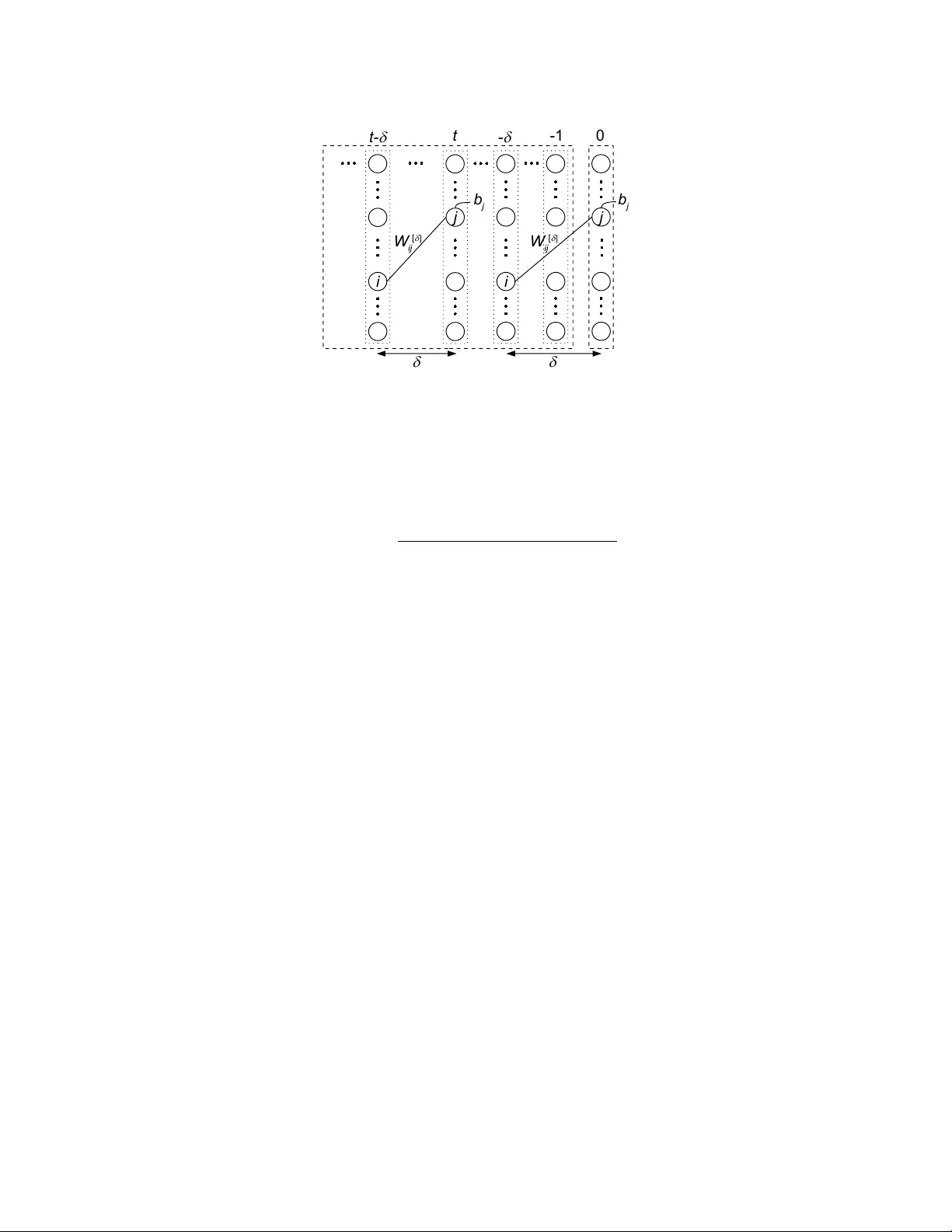
September 28, 2015 RT0967 Mathematics 13 pages Resear ch Report Learning dynamic Boltzmann machines with spik e-timing dependent plasticity T akayuki Osogami and Makoto Otsuka IBM Research - T okyo IBM Japan, Ltd. 19-21 Hakozaki, Chuo-ku, T okyo 103-8510, Japan Lear ning dynamic Boltzmann machines with spike-timing dependent plasticity T akayuki Osogami IBM Research - T okyo Makoto Otsuka IBM Research - T okyo Abstract W e propose a particularly structured Boltzmann machine, which we refer to as a dynamic Boltzmann machine (DyBM), as a stochastic model of a multi- dimensional time-series. The DyBM can have infinitely many layers of units but allows exact and ef ficient inference and learning when its parameters have a pro- posed structure. This proposed structure is motiv ated by postulates and observa- tions, from biological neural networks, that the synaptic weight is strengthened or weakened, depending on the timing of spikes (i.e., spike-timing dependent plas- ticity or STDP). W e show that the learning rule of updating the parameters of the DyBM in the direction of maximizing the likelihood of gi ven time-series can be interpreted as STDP with long term potentiation and long term depression. The learning rule has a guarantee of con vergence and can be performed in a distributed matter (i.e., local in space) with limited memory (i.e., local in time). 1 Introduction Boltzmann machines hav e seen successful applications in recognition of images and other tasks of machine learning [38, 32, 5, 4], particularly with recent dev elopment of deep learning [14]. The standard approaches to training a Boltzmann machine iterati vely apply a Hebbian rule [10] either exactly or approximately , where the v alues of the parameters are updated in the directions of in- creasing the likelihood of given training data with respect to the equilibrium distribution of the Boltzmann machine [15]. This Hebbian rule for the Boltzmann machine is limited in the sense that the concept of time is missing. For biological neural networks, spike-timing dependent plasticity (STDP) has been postulated and supported empirically [21, 2, 31]. For example, the synaptic weight is strengthened when a post-synaptic neuron fires shortly after a pre-synaptic neuron fires (i.e., long term potentiation) but is weak ened if this order of firing is rev ersed (i.e., long term depression). In this paper , we study the dynamics of a Boltzmann machine, or a dynamic Boltzmann machine (DyBM) 1 , and deri ve a learning rule for the DyBM that can be interpreted as STDP . While the con ventional Boltzmann machine is trained with a collection of static patterns (such as images), the DyBM is trained with a time-series of patterns. In particular , the DyBM gi ves the conditional probability of the next values (patterns) of a time-series given its historical v alues. This conditional probability can depend on the whole history of the time-series, and the DyBM can thus be used iterativ ely as a generativ e model of a time-series. Specifically , we define the DyBM as a Boltzmann machine having multiple layers of units, where one layer represents the most recent values of a time-series, and the remaining layers represent the historical values of the time-series. W e assume that the most recent values are conditionally independent of each other giv en the historical values. The DyBM allows an infinite number of layers, so that the most recent values can depend on the whole history of the time series. W e train the DyBM in such a way that the likelihood of gi ven time-series is maximized with respect to the 1 The natural acronym, DBM, is reserv ed for Deep Boltzmann Machines [29]. 2 conditional distribution of the next values given the historical values. This definition of the DyBM and the general approach to training the DyBM constitute the first contribution of this paper . W e show that the learning rule for the DyBM is significantly simplified and exhibits various char- acteristics of STDP that have been observ ed in biological neural networks [1], when the DyBM has an infinite number of layers and particularly structured parameters. Specifically , we assume that the weight between a unit representing a most recent v alue (time 0) and a unit representing the value in the past (time − t ) is the sum of geometric functions with respect to t . W e sho w that updating pa- rameters associated with a pair of units requires only the information that is av ailable at those units (i.e., local in space), and the required information can be maintained by k eeping a first-in-first-out (FIFO) queue of the last v alues of a unit (i.e., local in time). The con ver gence of the learning rule is guaranteed with sufficiently lo w learning rate, because the parameters are always updated such that the likelihood of gi ven training data is increased. The learning rule that is formally derived for the DyBM and its interpretation as STDP constitute the second contribution of this paper . The prior work has extended the Boltzmann machine to incorporate the timing of spikes in various ways [13, 33, 34, 36, 24]. Howe ver , the existing learning rules for those extended Boltzmann ma- chines in volve approximation with contrasti ve div ergence and do not ha ve some of the characteristics of the STDP (e.g., long term depression) that we show for the DyBM. W e will see that the DyBM can be considered as a recurrent neural network (RNN) equipped with memory units. The DyBM is thus related to Long Short T erm Memory [17, 7, 8, 6] and other RNNs [11, 26, 28, 22, 35]. What distinguishes the DyBM from e xisting RNNs is that training a DyBM does not require “backpropagation through time, ” or a chain rule of deriv ativ es. This distinguishing feature of the DyBM follows from the fact the DyBM can be equiv alently interpreted both as an RNN and as a non-recurrent Boltzmann machine. The learning rule deri ved from the interpretation as a non-recurrent Boltzmann machine clearly does not in volv e backpropagation through time b ut is a proper learning rule for the equiv alent RNN. As a result, training a DyBM is free from the “vanishing gradient problem” [16, 27]. The learning rule for some of the existing recurrent neural networks in v olves STDP but in a more limited form than our learning rule. For example, the learning rule of [26] depends on the timing of spikes but only on whether a post-synaptic neuron fires immediately after a pre-synaptic neuron fires. In our learning rule, the magnitude of the changes in the weight can depend on the dif ference between the timings of the two spikes, as has been observ ed for biological neural networks [1]. An extended version of this paper has appeared in [25]. This paper, howe ver , contains some of the details and perspectives that are omitted from [25]. Also, note that the notations and terminologies in this paper are not necessarily consistent with those in [25]. 2 Defining dynamic Boltzmann machine After re viewing the Boltzmann machine and the restricted Boltzmann machine in Section 2.1, we define the DyBM in Section 2.2. A learning rule for the DyBM and its interpretation as STDP will be provided in Section 3. 2.1 Con ventional Boltzmann machine A Boltzmann machine is a network of units that are mutually connected with weight (see Fig- ure 1 (a)). Let N be the number of units. For i ∈ [1 , N ] , let x i be the v alue of the i -th unit, where x i ∈ { 0 , 1 } . Let w i,j be the weight between the i -th unit and the j -th unit for i, j ∈ [1 , N ] . It is standard to assume that w i,i = 0 and w i,j = w j,i for i, j ∈ [1 , N ] . For i ∈ [1 , N ] , the bias, b i , is associated with the i -th unit. W e use the following notations of column vectors and matrices: x ≡ ( x i ) i ∈ [1 ,N ] , b ≡ ( b i ) i ∈ [1 ,N ] , and W ≡ ( w i,j ) i,j ∈ [1 ,N ] 2 . Let θ ≡ ( b , W ) denote the parameters of the Boltzmann machine. The energy of the v alues, x , for the N units of the Boltzmann machine having θ is given by E θ ( x ) = − b > x − 1 2 x > W x . (1) 3 j i W i j (a) Boltzmann machine W i j [1 ] j i (b) RBM W i j [ d ] j i (c) DyBM Figure 1: (a) A Boltzmann machine, (b) a restricted Boltzmann machine, and (c) a DyBM. The (equilibrium) probability of generating particular values, x , is giv en by P θ ( x ) = exp  − τ − 1 E θ ( x )  P ˜ x exp ( − τ − 1 E θ ( ˜ x )) , (2) where the summation over ˜ x denotes the summation over all of the possible configurations of a binary vector of length N , and τ is the parameter called temperature. The Boltzmann machine can be trained in the direction of maximizing the log likelihood of a giv en set, D , of the v ectors of the values: ∇ θ log P θ ( D ) = X x ∈D ∇ θ log P θ ( x ) , (3) where P θ ( D ) ≡ Q x ∈D P θ ( x ) , and ∇ θ log P θ ( x ) = − τ − 1  ∇ θ E θ ( x ) − X ˜ x P θ ( ˜ x ) ∇ θ E θ ( ˜ x )  . (4) A Hebbian rule can be derived from (4). For example, to increase the likelihood of a data point, x , we should update W i,j by W i,j ← W i,j + η ( x i x j − h X i X j i θ ) , (5) where h X i X j i θ denotes the expected v alue of the product of the values of the i -th unit and the j -th unit with respect to P θ in (2), and η is a learning rate [15]. A particularly interesting case is a restricted Boltzmann machine (RBM), where the units are divided into two layers, and there is no weight between the units in each layer (see Figure 1 (b)). In this case, P θ ( x ) can be e valuated approximately with contrastive diver gence [12, 30] or other methods [37, 3] when the exact computation of (4) is intractable (e.g., when N is large). A ke y property of the RBM that allo ws contrasti ve di vergence is the following conditional indepen- dence. F or t ∈ [1 , 2] , let x [ t ] be the v alues of the units in the t -th layer and b [ t ] be the corresponding bias. Let W [1] be the matrix whose ( i, j ) element is the weight between the i -th unit in the first layer and the j -th unit in the second layer . Then the conditional probability of x [2] giv en x [1] is giv en by P θ ( x [2] | x [1] ) = Y j ∈ [1 ,N ] P θ,j ( x [2] j | x [1] ) (6) ≡ Y j ∈ [1 ,N ] exp  − τ − 1 E θ,j ( x [2] j | x [1] )  X x [2] j ∈{ 0 , 1 } exp  − τ − 1 E θ,j ( x [2] j | x [1] )  , (7) where P θ,j ( x [2] j | x [1] ) denotes the conditional probability that the j -th unit of the second layer has value x [2] j giv en that the first layer has values x [1] , and we define E θ,j ( x [2] j | x [1] ) ≡ − b j x [2] j − ( x [1] ) > W [1] : ,j x [2] j , (8) 4 where W [1] : ,j denotes the j -th column of W [1] . Namely , the value of the units in the second layer , x [2] , is conditionally independent of each other giv en x [1] . 2.2 Dynamic Boltzmann machine W e propose the dynamic Boltzmann machine (DyBM), which can hav e infinitely many layers of units (see Figure 1 (c)). Similar to the RBM, the DyBM has no weight between the units in the right-most layer of Figure 1 (c). Unlike the RBM, each layer of the DyBM has a common number , N , of units, and the bias and the weight in the DyBM can be shared among dif ferent units in a particular manner . Formally , we define the DyBM- T as the Boltzmann machine having T layers from − T + 1 to 0 , where T is a positiv e integer or infinity . Let x ≡ ( x [ t ] ) − T 2 as a ( T − 1) -st order Markov model, where the next values are conditionally independent of the history gi ven the v alues of the last ( T − 1) steps. W ith a DyBM- ∞ , the next values can depend on the whole history of the time-series. In principle, the DyBM- ∞ can thus model any time-series possibly with long-term dependency , as long as the values of the time-series at a moment is conditionally independent of each other giv en its values preceding that moment. Using the conditional probability giv en by a DyBM- T , the probability of a sequence, x = x ( − L, 0] , of length L is giv en by p ( x ) = 0 Y t = − L +1 P θ ( x [ t ] | x ( t − T , : t − 1] ) , (9) where we arbitrarily define x [ t ] ≡ 0 for t ≤ − L . Namely , the v alues are set zero if there are no corresponding history . 3 Spike-timing dependent plasticity W e deri ve a learning rule for a DyBM- T in such a way that the log likelihood of a given (set of) time-series is maximized. W e will see that the learning rule is particularly simplified in the limit of T → ∞ when the parameters of the DyBM- ∞ have particular structures. W e will show that this learning rule exhibits v arious characteristics of spike-timing dependent plasticity (STDP). 3.1 General learning rule of dynamic Boltzmann machines The log lik elihood of a giv en set, D , of time-series can be maximized by maximizing the sum of the log likelihood of x ∈ D . By (9), the log likelihood of x = x ( − L, 0] has the following gradient: ∇ θ log p ( x ) = 0 X t = − L +1 ∇ θ log P θ ( x [ t ] | x ( t − T ,t − 1] ) . (10) 5 d i j W i j [ d ] ^ - d j i W j i [ - d ] ^ W i j [ d ] d w ei gh t Figure 2: The figure illustrates Equation (12) with particular forms of Equation (13). The horizontal axis represents δ , and the vertical axis represents the value of W [ δ ] i,j (solid curves), ˆ W [ δ ] i,j (dashed curves), or ˆ W [ − δ ] j,i (dotted curves). Notice that W [ δ ] i,j is defined for δ > 0 and is discontinuous at δ = d i,j . On the other hand, ˆ W [ δ ] i,j and ˆ W [ − δ ] j,i are defined for −∞ < δ < ∞ and discontinuous at δ = d i,j and δ = − d j,i , respectiv ely . W e can thus exploit the conditional independence of (7) to deri ve the learning rule: ∇ θ log P θ ( x [0] | x ( − T , − 1] ) = − τ − 1 X j ∈ [1 ,N ]  ∇ θ E θ,j ( x [0] j | x ( − T , − 1] ) − X ˜ x [0] j ∈{ 0 , 1 } P θ,j ( ˜ x [0] j | x ( − T , − 1] ) ∇ θ E θ,j ( ˜ x [0] j | x ( − T , − 1] )  . (11) One could, for example, update θ in the direction of (11) every time new x [0] is observed, using the latest history , x ( − T , − 1] . This is an approach of stochastic gradient. In practice, howe ver , the computation of (11) can be intractable for a large T , because there are Θ( M T ) parameters to learn, where M is the number of the pairs of connected units ( M = Θ( N 2 ) when all of the units are densely connected). 3.2 Deriving a specific learning rule W e thus propose a particular form of weight sharing, which is motivated by observations from biological neural networks [1] but leads to particularly simple, exact, and efficient learning rule. In biological neural networks, STDP has been postulated and supported experimentally . In particular , the synaptic weight from a pre-synaptic neuron to a post-synaptic neuron is strengthened, if the post-synaptic neuron fires (generates a spike) shortly after the pre-synaptic neuron fires (i.e., long term potentiation or L TP). This weight is weakened, if the post-synaptic neuron fires shortly befor e the pre-synaptic neuron fires (i.e., long term depression or L TD). These dependenc y on the timing of spikes is missing in the Hebbian rule for the Boltzmann machine (5). T o derive a learning rule that has the characteristics of STDP with L TP and L TD, we consider the weight of the form illustrated in Figure 2. For δ > 0 , we define the weight, W [ δ ] i,j , as the sum of two weights, ˆ W [ δ ] i,j and W [ − δ ] j,i : W [ δ ] i,j = ˆ W [ δ ] i,j + ˆ W [ − δ ] j,i . (12) 6 In Figure 2, the value of ˆ W [ δ ] i,j is high when δ = d i,j , the (synaptic) delay from i -th (pre-synaptic) unit to the j -th (post-synaptic) unit. Namely , the post-synaptic neuron is likely to fire (i.e., x [0] j = 1 ) immediately after the spike from the pre-synaptic unit arrives with the delay of d i,j (i.e, x [ − d i,j ] i = 1 ). This likelihood is controlled by the magnitude of ˆ W [ d i,j ] i,j , which we will learn from training data. The value of ˆ W [ δ ] i,j gradually decreases, as δ increases from d i,j . That is, the effect of the stimulus of the spike arri ved from the i -th unit diminishes with time [1]. The v alue of ˆ W [ d i,j − 1] i,j is lo w , suggesting that the post-synaptic unit is unlikely to fire (i.e., x [0] j = 1 ) immediately before the spike from the i -th (pre-synaptic) unit arri ves. This unlikelihood is controlled by the magnitude of ˆ W [ d i,j − 1] i,j , which we will learn. As δ decreases from d i,j − 1 , the magnitude of ˆ W [ δ ] i,j gradually decreases [1]. Here, δ can get smaller than 0, and ˆ W [ δ ] i,j with δ < 0 represents the weight between the spike of the pre-synaptic neuron that is generated after the spike of the post-synaptic neuron. The assumption of W [0] i,j = 0 is con venient for computational purposes but can be justified in the limit of infinitesimal time steps. Specifically , consider a scaled DyBM where both the step size of the time and the probability of firing are made 1 /n -th of the original DyBM. In the limit of n → ∞ , the scaled DyBM has continuous time, and the probability of having simultaneous spikes from two units tends to zero. For tractable learning and inference, we assume the follo wing form of weight: ˆ W [ δ ] i,j =            0 if δ = 0 X k ∈K u i,j,k λ δ − d i,j k if δ ≥ d i,j X ` ∈L − v i,j,` µ − δ ` otherwise (13) where λ k , µ ` ∈ (0 , 1) for k ∈ K and ` ∈ L . W e will learn the v alues of u i,j,k and v i,j,` based on training dataset. W e assume that λ k for k ∈ K , µ ` for ` ∈ L , and d i,j for i, j ∈ [1 , N ] are giv en (or need to be learned as h yper-parameters). With an analogy to biological neural netw orks, these gi ven parameters ( λ k , µ ` , and d i,j ) are determined based on physical constraints or chemical properties, while the weight ( u i,j,k and v i,j,` ) and the bias ( b ) are learned based on the neural spikes ( x ). The sum of geometric functions with v arying decay rates [19] in (13) is moti vated by long-term memory (or dependency) [23, 34]. See Figure 3 for the flexibility of the sum of geometric functions. In particular , the sum of geometric functions can well approximate a hyperbolic function, whose v alue decays more slowly than any geometric functions. This slow decay is considered to be essential for long-term memory . Howe ver , our results also hold for the simple cases where |K | = |L| = 1 . W ith the abov e specifications and letting T → ∞ , we can now represent the E θ,j ( x [0] j | x ( − T , − 1] ) appearing in (11) as follows: E θ,j ( x [0] j | x ( −∞ , − 1] ) = − b j x [0] j − − 1 X t = −∞ ( x [ t ] ) > W [ − t ] : ,j x [0] j , (14) where W [ − t ] : ,j ≡  W [ − t ] i,j  i =1 ,...,N denotes a column vector . By (12) and (13), the second term of (14) is giv en by − 1 X t = −∞ ( x [ t ] ) > W [ − t ] : ,j x [0] j = N X i =1  X k ∈K u i,j,k α i,j,k − X ` ∈L v i,j,` β i,j,` − X ` ∈L v j,i,` , γ i,`  x [0] j (15) 7 0 5 10 15 20 25 30 t 1 0 - 3 1 0 - 2 1 0 - 1 1 0 0 Figure 3: The solid curve shows the sum of three geometric functions ( 10 − 0 . 3 t , 10 − 0 . 1 t − 1 , and 10 − 0 . 1 t/ 3 − 2 ) shown with dotted lines (the v ertical axis is in the log scale). where α i,j,k , β i,j,` , and γ i,` are the quantities, which we refer to as eligibility traces, that depend on x ( −∞ , − 1] i , the history of the i -th unit: α i,j,k ≡ − d i,j X t = −∞ λ − t − d i,j k x [ t ] i ; (16) β i,j,` ≡ − 1 X t = − d i,j +1 µ t ` x [ t ] i ; (17) γ i,` ≡ − 1 X t = −∞ µ − t ` x [ t ] i . (18) W e now deri ve the deri v atives of (14), which we need for (11), as follo ws: ∂ ∂ b j E θ,j ( x [0] j | x ( −∞ , − 1] ) = − x [0] j , (19) ∂ ∂ u i,j,k E θ,j ( x [0] j | x ( −∞ , − 1] ) = − α i,j,k x [0] j , (20) ∂ ∂ v i,j,` E θ,j ( x [0] j | x ( −∞ , − 1] ) = β i,j,` x [0] j , (21) ∂ ∂ v j,i,` E θ,j ( x [0] j | x ( −∞ , − 1] ) = γ i,` x [0] j . (22) By plugging the abov e deriv ativ es into (11), we have, for i, j ∈ [1 , N ] , k ∈ K , and ` ∈ L , that ∂ ∂ b j log P θ ( x [0] | x ( −∞ , − 1] ) = τ − 1  x [0] j − h X [0] j i θ  (23) ∂ ∂ u i,j,k log P θ ( x [0] | x ( −∞ , − 1] ) = τ − 1 α i,j,k  x [0] j − h X [0] j i θ  (24) ∂ ∂ v i,j,` log P θ ( x [0] | x ( −∞ , − 1] ) = − τ − 1 β i,j,`  x [0] j − h X [0] j i θ  − τ − 1 γ j,`  x [0] i − h X [0] i i θ  , (25) 8 W i j [ d ] j i i W i j [ d ] b j d 0 - 1 - d t- d j b j d t Figure 4: The homogeneous DyBM. where h X [0] j i θ denotes the expected value of the j -th unit in the 0-th layer of the DyBM- ∞ gi ven the history x ( −∞ , − 1] . Because the v alue is binary , this expected value is gi ven by h X [0] j i θ = P θ,j (1 | x ( −∞ , − 1] ) (26) = exp  − τ − 1 E θ,j (1 | x ( −∞ , − 1] )  1 + exp  − τ − 1 E θ,j (1 | x ( −∞ , − 1] )  , (27) which can be calculated, using the eligibility traces in (16)-(18). Here, the first term of the denomi- nator of (27) is 1, because E θ,j (0 | x ( −∞ , − 1] ) = 0 . T o maximize the likelihood of a giv en set, D , of sequences, the parameters θ can be updated with θ ← θ + η X x ∈D ∇ θ log P θ ( x [0] | x ( −∞ , − 1] ) . (28) T ypically , a single time-series, y [1 ,L ] , is av ailable for training the DyBM- ∞ . In this case, we form D ≡ { y [1 ,t ] | t ∈ [1 , L ] } , where y [1 ,t ] is used as x [0] ≡ y [ t ] and x ( −∞ , − 1] ≡ y ( −∞ ,t − 1] , where recall that we arbitrarily set zeros when there are no history (i.e., y [ t ] ≡ 0 for t ≤ 0 ). When D is made from a single time-series, the eligibility traces (16)-(18) needed for training with y [1 ,t ] can be computed recursiv ely from the ones used for y [1 ,t − 1] . In particular , we ha ve α i,j,k ← λ k  α i,j,k + y [ t − d i,j ] i  (29) γ i,` ← µ `  γ i,` + y [ t − 1] i  . (30) This recursiv e calculation requires keeping the follo wing FIFO queue of length d i,j − 1 : q i,j ≡  y [ t − 2] i , . . . , y [ t − d i,j +1] i , y [ t − d i,j ] i  (31) for each i, j ∈ [1 , N ] . After training with y [1 ,t − 1] , the q i,j is updated by adding y [ t − 1] i and delet- ing y [ t − d i,j ] i . The remaining eligibility trace β i,j,` can be calculated non-recursi vely by the use of q i,j . In fact, our experience suggests that a recursiv e calculation of β i,j,k is amenable to numerical instability , so that β i,j,k should be calculated non-recursiv ely . 3.3 Homogeneous dynamic Boltzmann machine Here, we will show that the DyBM- ∞ can indeed be understood as a generati ve model of a time series. For this purpose, we will specify the bias for the units in the s -th layer for s ≤ − 1 and the weight between the units in the s -th layer and the units in the t -th layer , for s, t ≤ − 1 . Recall that 9 y i [ t ] y i [ t - 1 ] y i [ t - 2] y i [ t - d i j - 1] Neuron i N e uron j t g i , l b i , j , l t a i , j , k Figure 5: Spikes trav eling from a pre-synaptic neuron ( i ) to a post-synaptic neuron ( j ) and eligibility traces. these bias and weight hav e not been specified in the discussion so f ar, because they do not af fect the conditional probability: P θ ( x [0] | x ( −∞ , − 1] ) . (32) This model of a single time step with (32) is used iterativ ely in (9) to define the distribution of a time series. Strictly speaking, howe ver , this iterativ e use of (32) is not a generativ e model defined solely with a Boltzmann machine. W e now consider the following homogeneous DyBM (see Figure 4), which is a special case of a DyBM- ∞ . Let each layer of the units has a common vector of bias. That is, for any s , the units in the s -th layer have the bias, b . Let the matrix of the weight between tw o layers, s and t , depend only on the distance, t − s , between the two layers. That is, for an y pair of s and t , the i -th unit in the s -th layer and the j -th unit in the t -th layer is connected with the weight, W [ t − s ] i,j , for i, j ∈ [1 , N ] . The learning rule deriv ed for the DyBM- ∞ in Section 3.1 - Section 3.2 holds for the homogeneous DyBM. The key property of the homogeneous DyBM is that the homogeneous DyBM consisting of the layers up to the t -th layer , for t < 0 , is equi valent to the homogeneous DyBM consisting of the layers up to the 0 -th layer . Therefore, the iterative use of the model of the single time step (32) is now equi v alent to the generative model of a time-series defined with a single homogeneous DyBM. Specifically , the values of the time-series at time t are generated based on the conditional probability , P θ ( x [ t ] | x ( −∞ ,t − 1] ) , that is given by the homogeneous DyBM consisting of the layers up to the t - th layer . The values, x [ t ] , generated at time t are then used as a part of the history x ( −∞ ,t ] for the homogeneous DyBM consisting of the layers up to the ( t + 1) -st layer , which in turn defines the conditional probability of the values at time t + 1 . The homogeneous DyBM can also have the layers for positive time steps ( t > 0 ). The homogeneous DyBM can then be interpreted as a recurrent neural network, which we will discuss in the following with reference to an artificial neural network. 3.4 Interpr etation as an artificial neural network Figure 5 illustrates the learning rule deriv ed in Section 3.1-Section 3.2 from a point of artificial neural netw orks. Consider a pre-synaptic neuron, i , and a post-synaptic neuron, j . The FIFO queue, q i,j , can be considered as an axon that stores the spikes traveling from i to j . The conduction delay of this axon is d i,j , and the spikes generated in the last d i,j − 1 steps are stored. The spikes in the axon determine the value of β i,j,` for each ` ∈ L . Another eligibility trace, γ i,` , records the aggregated information about the spikes generated at the neuron i , where the spikes generated in the past are discounted with the rate that depends on ` ∈ L . The remaining eligibility trace, α i,j,k , records the aggregated information about the spikes that hav e reached j from i , where the spikes arriv ed in the past are discounted with the rate that depends on k ∈ K . The DyBM- ∞ can then be considered as a recurrent neural network, taking binary values, equipped with memory units that store eligibility traces and the FIFO queue (see Figure 6). For learning or inference with an N -dimensional binary time-series of arbitrary length, this recurrent neural network 10 i q i j a i j k j g i l b i j l Figure 6: The homogeneous DyBM as a recurrent neural network with memory . needs the working space of O ( N + M D ) binary bits and O ( M |K | + M |L| ) floating-point numbers, where M is the number of ordered pairs of connected units (i.e, the number of the pairs of i and j such that W [ δ ] i,j 6 = 0 for a δ ≥ 1 in the DyBM- ∞ ), and D is the maximum delay such that d i,j ≤ D . Specifically , the binary bits correspond to the N bits of x [0] and M FIFO queues. The floating-point numbers correspond to eligibility traces ( α i,j,k and γ i,k for i, j ∈ [1 , N ] , k ∈ K , and ` ∈ L ), the coefficients of the weight ( u i,j,k and v i,j,` for i, j ∈ [1 , N ] , k ∈ K , and ` ∈ L ), and the bias ( b j for j ∈ [1 , N ] ). Each of the parameters of the DyBM- ∞ can be updated in a distrib uted manner by the use of the learning rules from (23)-(25). Observe that this distributed update can be performed in constant time that is independent of N , D , |K| , and |L| . According to (27) and (14), the neuron j is more likely to fire ( x [0] j = 1 ) when (i) b j is high, (ii) u i,j,k and α i,j,k are high, or (iii) both conditions are met. The learning rule (23) suggests that b j increases ov er time, if the neuron j fires more often than it is e xpected from the latest v alues of the parameters of the DyBM- ∞ . The learning rule (24) suggests that u i,j,k increases over time, if the neuron j fires more often than it is expected, and the magnitude of the changes in u i,j,k is proportional to the magnitude of α i,j,k . These implement long term potentiation. According to (27) and (14), the neuron j is less likely to fire when (i) v i,j,` and β i,j,` are high, (ii) v j,i,` and γ i,` are high, (iii) or both conditions are met. The learning rule (25) suggests that v i,j,k increases over time, if the neuron j fires less often than it is expected, and the magnitude of the changes in v i,j,k is proportional to the magnitude of β i,j,` . When i and j are e xchanged, the learning rule (25) suggests that v i,j,k increases ov er time, if the neuron j fires less often than it is expected, and the magnitude of the changes in v i,j,k is proportional to the magnitude of γ i,` . These implement long term depression. Here, the terms in (23)-(25) that inv olve expected v alues (27) can be considered as a mechanism of homeostatic plasticity [20] that keeps the firing probability relatively constant. This particular mechanism of homeostatic plasticity does not appear to ha ve been discussed with STDP in the liter - ature [20, 39]. W e expect, howe ver , that this formally deri ved mechanism of homeostatic plasticity plays an essential role in stabilizing the learning of artificial neural networks. W ithout this homeo- static plasticity , the values of the parameters can indeed di verge or fluctuate during training. 4 Conclusion Our work provides theoretical underpinnings on the postulates about STDP . Recall that the Hebb rule was first postulated in the middle of the last century [10] b ut had seen limited success in engineering applications until more than 30 years later when the Hopfield network [18] and the Boltzmann machine [15] are used to pro vide theoretical underpinnings. In particular , a Hebbian rule w as sho wn to increase the likelihood of data with respect to the distribution associated with the Boltzmann machine [15]. STDP has been postulated for biological neural networks and has been used for artificial neural networks but in rather ad hoc ways. Our work establishes the relation between STDP and the Boltzmann machine for the first time in a formal manner . Specifically , we propose the DyBM as a stochastic model of time-series. The DyBM gives the conditional probability of the next values of a multi-dimensional time-series giv en its historical values. This conditional probability can depend on the whole history of arbitrary length, so that the 11 DyBM (specifically , DyBM- ∞ ) does not hav e the limitation of a Marko v model or a higher order Markov model with a finite order . The conditional probability given by the DyBM- ∞ can thus be applied recursi vely to obtain the probability of generating a particular time-series of arbitrary length. The DyBM- ∞ can be trained in a distrib uted manner (i.e., local in space) with limited memory (i.e., local in time) when its parameters have a proposed structure. The learning rule is local in space in that the parameters associated with a pair of the units in the DyBM- ∞ can be updated by using only the information that is av ailable locally in those units. The learning rule is local in time in that it requires only a limited length of the history of a time-series. This training is guaranteed to con verge as long as the learning rate is set sufficiently small. The DyBM- ∞ having the proposed structure (i.e., the homogeneous DyBM) can be considered as a recurrent neural netw ork, taking binary v alues, with memory units (or a recurrent Boltzmann machine with memory). Specifically , each neuron stores eligibility traces and updates their values based on the spikes that it generates and the spikes received from other neurons. An axon stores spikes that trav el from a pre-synaptic neuron to a post-synaptic neuron. The synaptic weight is updated e very moment, depending on the spikes that are generated at that moment and the values of these eligibility traces and the spikes stored in the axon. This learning rule exhibits various characteristics of STDP , including long term potentiation and long term depression, which have been postulated and observ ed empirically in biological neural networks. The learning rule also exhibits a form of homeostatic plasticity that is similar to those studied for Bayesian spiking networks (e.g., [9]). Howe ver , the Bayesian spiking network is a mixture-of-expert model, which is a particular type of a directed graphical model, while we study a product-of-expert model, which is a particular type of an undirected graphical model. W e expect that the theoretical underpinnings on STDP provided in this paper will accelerate engi- neering applications of STDP . In particular , the prior work [13, 33, 34, 36] has proposed various extensions of the Boltzmann machine to deal with time-series data, but existing learning algorithms for these extended Boltzmann machines in volv e approximations. On the other hand, the homoge- neous DyBM can be considered as a recurrent Boltzmann machine with memory , which naturally extends the Boltzmann machine (at the equilibrium state) by taking into account the dynamics and by incorporating the memory . STDP is to the DyBM what the Hebb rule is to the Boltzmann machine. Acknowledgements This research was supported by CREST , JST . References [1] L. F . Abbott and S. B. Nelson. Synaptic plasticity: Taming the beast. Natur e neur oscience , 3:1178–1183, 2000. [2] G. Bi and M. Poo. Synaptic modifications in cultured hippocampal neurons: Dependence on spik e timing, synaptic strength, and postsynaptic cell type. The Journal of Neur oscience , 18(24):10464–10472, 1998. [3] K. Cho, T . Raiko, and A. Ilin. Enhanced gradient and adaptive learning rate for training re- stricted Boltzmann machines. In Pr oceedings of the 28th Annual International Confer ence on Machine Learning (ICML 2011) , pages 105–112, 2011. [4] G. E. Dahl, R. P . Adams, and H. Larochelle. Training restricted Boltzmann machines on word observations. In Pr oceedings of the 29th Annual International Confer ence on Machine Learning (ICML 2012) , pages 679–686, 2012. [5] K. Georgie v and P . Nakov . A non-IID framew ork for collaborativ e filtering with restricted Boltzmann machines. In Pr oceedings of the 30th Annual International Conference on Mac hine Learning (ICML 2013) , pages 1148–1156, 2013. [6] A. Graves and N. Jaitly . T owards end-to-end speech recognition with recurrent neural net- works. In Proceedings of the 31st Annual International Conference on Machine Learning (ICML 2014) , pages 1764–1772, 2014. 12 [7] A. Graves, M. Liwicki, H. Bunke, J. Schmidhuber , and S. Fern ´ andez. Unconstrained on-line handwriting recognition with recurrent neural networks. In Advances in Neural Information Pr ocessing Systems 20 , pages 577–584. 2008. [8] A. Grav es and J. Schmidhuber . Offline handwriting recognition with multidimensional re- current neural networks. In Advances in Neural Information Pr ocessing Systems 21 , pages 545–552. 2009. [9] S. Habenschuss, J. Bill, and B. Nessler . Homeostatic plasticity in Bayesian spiking networks as expectation maximization with posterior constraints. In Advances in Neural Information Pr ocessing Systems, 25 , pages 782–790, 2012. [10] D. O. Hebb. The or ganization of behavior: A neur opsychological appr oach . John Wile y & Sons, 1949. [11] M. Hermans and B. Schrauwen. Training and analysing deep recurrent neural networks. In Advances in Neural Information Pr ocessing Systems 26 , pages 190–198. 2013. [12] G. E. Hinton. Training products of experts by minimizing contrastiv e di vergence. Neural computation , 14(8):1771–1800, 2002. [13] G. E. Hinton and A. D. Bro wn. Spiking Boltzmann machines. In Advances in Neural Infor- mation Pr ocessing Systems , pages 122–128, 1999. [14] G. E. Hinton and R. R. Salakhutdinov . Reducing the dimensionality of data with neural net- works. Science , 313(5786):504–507, 2006. [15] G. E. Hinton and T . J. Sejno wski. Optimal perceptual inference. In Pr oceedings of the IEEE confer ence on Computer V ision and P attern Recognition , pages 448–453, 1983. [16] S. Hochreiter , Y . Bengio, P . Frasconi, and J. Schmidhuber . Gradient flow in recurrent nets: The difficulty of learning long-term dependencies. In A Field Guide to Dynamical Recurr ent Neural Networks . IEEE Press, 2001. [17] S. Hochreiter and J. Schmidhuber . Long short-term memory . Neural Computation , 9(8):1735– 1780, 1997. [18] J. J. Hopfield. Neural networks and physical systems with emergent collecti ve computational abilities. Pr oceedings of the National Academy of Sciences , 79(8):2554–2558, 1982. [19] P . R. Killeen. Writing and overwriting short-term memory . Psychonomic Bulletin & Review , 8:18–43, 2001. [20] A. Lazar , G. Pipa, and J. T riesch. SORN: A self-organizing recurrent neural netw ork. F r ontiers in Computational Neur oscience , 3, 2009. [21] H. Markram, J. L ¨ ubke, M. Frotscher , and B. Sakmann. Regulation of synaptic efficac y by coincidence of postsynaptic APs and EPSPs. Science , 275(5297):213–215, 1997. [22] J. Martens and I. Sutskev er . Learning recurrent neural networks with Hessian-free optimiza- tion. In Pr oceedings of the 28 th International Confer ence on Mac hine Learning (ICML 2011) , pages 1033–1040, 2011. [23] D. McCarthy and K. G. White. Behavioral models of delayed detection and their applilcation to the study of memory . In The Effect of Delay and of Intervening Events on Reinforcement V alue: Quantitative Analyses of Behavior , V olume V , chapter 2. Psychology Press, 2013. [24] R. Mittelman, B. Kuipers, S. Sav arese, and H. Lee. Structured recurrent temporal restricted Boltzmann machines. In Pr oceedings of the 31st Annual International Confer ence on Machine Learning (ICML 2014) , pages 1647–1655, 2014. [25] T . Osogami and M. Otsuka. Se ven neurons memorizing sequences of alphabetical images via spike-timing dependent plasticity . Scientific Reports , 5:14149, 2015. doi: 10.1038/srep14149. [26] M. Pachitariu and M. Sahani. Learning visual motion in recurrent neural networks. In Advances in Neural Information Pr ocessing Systems 25 , pages 1322–1330. 2012. [27] R. Pascanu, T . Mik olov , and Y . Bengio. On the difficulty of training recurrent neural netw orks. In Proceedings of the 30th Annual International Confer ence on Machine Learning (ICML 2013) , pages 1310–1318, 2013. 13 [28] P . H. O. Pinheiro and R. Collobert. Recurrent con volutional neural networks for scene label- ing. In Pr oceedings of the 31st Annual International Confer ence on Mac hine Learning (ICML 2014) , pages 82–90, 2014. [29] R. Salakhutdinov and G. E. Hinton. Deep Boltzmann machines. In Pr oceedings of the Inter- national Confer ence on Artificial Intelligence and Statistics , volume 5, pages 448–455, 2009. [30] R. Salakhutdinov , A. Mnih, and G. E. Hinton. Restricted Boltzmann machines for collaborati ve filtering. In Pr oceedings of the 24th Annual International Conference on Machine Learning (ICML 2007) , pages 791–798, 2007. [31] P . J. Sj ¨ ostr ¨ om, G. G. T urrigiano, and S. B. Nelson. Rate, timing, and cooperativity jointly determine cortical synaptic plasticity . Neuron , 32(6):1149–1164, 2001. [32] K. Sohn, G. Zhou, C. Lee, and H. Lee. Learning and selecting features jointly with point-wise gated Boltzmann machines. In Pr oceedings of the 30th Annual International Confer ence on Machine Learning (ICML 2013) , pages 217–225, 2013. [33] I. Sutske ver and G. E. Hinton. Learning multilevel distributed representations for high- dimensional sequences. In International Conference on Artificial Intelligence and Statistics , pages 548–555, 2007. [34] I. Sutske ver , G. E. Hinton, and G. W . T aylor . The recurrent temporal restricted Boltzmann machine. In Advances in Neural Information Pr ocessing Systems , pages 1601–1608, 2008. [35] I. Sutske ver , J. Martens, and G. E. Hinton. Generating text with recurrent neural networks. In Pr oceedings of the 28 th International Confer ence on Machine Learning (ICML 2011) , pages 1017–1024, 2011. [36] G. W . T aylor and G. E. Hinton. Factored conditional restricted Boltzmann machines for mod- eling motion style. In Pr oceedings of the 26th Annual International Confer ence on Machine Learning (ICML 2009) , pages 1025–1032, 2009. [37] T . T ieleman. Training restricted boltzmann machines using approximations to the likelihood gradient. In Pr oceedings of the 25th Annual International Confer ence on Machine Learning (ICML 2008) , pages 1064–1071, 2008. [38] T . T ran, D. Q. Phung, and S. V enkatesh. Thurstonian Boltzmann machines: Learning from multiple inequalities. In Pr oceedings of the 30th Annual International Confer ence on Machine Learning (ICML 2013) , pages 46–54, 2013. [39] G. G. T urrigiano and S. B. Nelson. Homeostatic plasticity in the developing nervous system. Natur e Reviews Neur oscience , 5(2):97–107, 2004. 14