Minimum Weight Perfect Matching via Blossom Belief Propagation

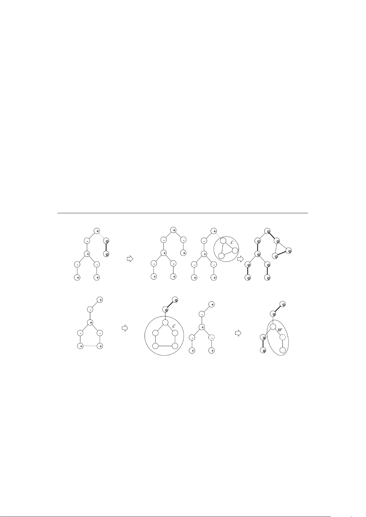
Minimum W eight Perfect Matching via Blossom Belief Propagation Sungsoo Ahn, Sejun Park, Michael Chertk ov ∗ , Jinwoo Shin † September 24, 2015 Abstract Max-product Belief Propagation (BP) is a popular message-passing algorithm for computing a Maximum-A-Posteriori (MAP) assignment ov er a distribution represented by a Graphical Model (GM). It has been sho wn that BP can solve a number of combinato- rial optimization problems including minimum weight matching, shortest path, network flow and verte x cov er under the following common assumption: the respecti ve Linear Programming (LP) relaxation is tight, i.e., no integrality gap is present. Howe ver , when LP shows an integrality gap, no model has been known which can be solved systemati- cally via sequential applications of BP . In this paper, we de velop the first such algorithm, coined Blossom-BP , for solving the minimum weight matching problem ov er arbitrary graphs. Each step of the sequential algorithm requires applying BP o ver a modified graph constructed by contractions and expansions of blossoms, i.e., odd sets of vertices. Our scheme guarantees termination in O ( n 2 ) of BP runs, where n is the number of vertices in the original graph. In essence, the Blossom-BP offers a distrib uted v ersion of the cel- ebrated Edmonds’ Blossom algorithm by jumping at once over many sub-steps with a single BP . Moreover , our result provides an interpretation of the Edmonds’ algorithm as a sequence of LPs. 1 Intr oduction Graphical Models (GMs) provide a useful representation for reasoning in a number of scien- tific disciplines [ 1 , 2 , 3 , 4 ]. Such models use a graph structure to encode the joint probability distribution, where v ertices correspond to random variables and edges specify conditional de- pendencies. An important inference task in many applications inv olving GMs is to find the most-likely assignment to the variables in a GM, i.e., Maximum-A-Posteriori (MAP). Belief Propagation (BP) is a popular algorithm for approximately solving the MAP inference problem and it is an iterati ve, message passing one that is exact on tree structured GMs. BP often shows remarkably strong heuristic performance beyond trees, i.e., o ver loop y GMs. Furthermore, BP is of a particular relev ance to large-scale problems due to its potential for parallelization [ 5 ] and its ease of programming within the modern programming models for parallel computing, e.g., GraphLab [ 6 ], GraphChi [ 7 ] and OpenMP [ 8 ]. ∗ M. Chertkov is with the Theoretical Division at Los Alamos National Laboratory , USA. Author’ s e-mail: chertkov@lanl.gov † S. Ahn, S. Park and J. Shin are with the Department of Electrical Engineering at K orea Advanced Institute of Science T echnology , Republic of K orea. Authors’ e-mails: ssahn0215@kaist.ac.kr, sejun.park@kaist.ac.kr, jinwoos@kaist.ac.kr 1 The con ver gence and correctness of BP was recently established for a certain class of loopy GM formulations of sev eral classical combinatorial optimization problems, including matching [ 9 , 10 , 11 ], perfect matching [ 12 ], shortest path [ 13 ], independent set [ 14 ], network flo w [ 15 ] and vertex cover [ 16 ]. The important common feature of these models is that BP con verges to a correct assignment when the Linear Programming (LP) relaxation of the com- binatorial optimization is tight, i.e., when it sho ws no integrality gap. The LP tightness is an ine vitable condition to guarantee the performance of BP and no combinatorial optimization instance has been kno wn where BP w ould be used to solv e problems without the LP tightness. On the other hand, in the LP literature, it has been extensiv ely studied how to enforce the LP tightness via solving multiple intermediate LPs that are systematically designed, e.g., via the cutting-plane method [ 22 ]. Moti vated by these studies, we pose a similar question for BP , “ho w to enforce correctness of BP , possibly by solving multiple intermediate BPs”. In this pa- per , we show ho w to resolve this question for the minimum weight (or cost) perfect matching problem ov er arbitrary graphs. Contribution. W e de velop an algorithm, coined Blossom-BP , for solving the minimum weight matching problem over an arbitrary graph. Our algorithm solv es multiple interme- diate BPs until the final BP outputs the solution. The algorithm is sequential, where each step includes running BP ov er a ‘contracted’ graph deri ved from the original graph by contractions and infrequent expansions of blossoms, i.e., odd sets of vertices. T o build such a scheme, we first design an algorithm, coined Blossom-LP , solving multiple intermediate LPs. Second, we sho w that each LP is solvable by BP using the recent frame work [ 16 ] that establishes a generic connection between BP and LP . For the first part, cutting-plane methods solving multiple in- termediate LPs for the minimum weight matching problem ha ve been discussed by sev eral authors o ver the past decades [ 17 , 18 , 19 , 20 , 21 ] and a pro vably polynomial-time scheme w as recently suggested [ 22 ]. Ho we ver , LPs in [ 22 ] were quite complex to solve by BP . T o address the issue, we design much simpler intermediate LPs that allo w utilizing the framework of [ 16 ]. W e prove that Blossom-BP and Blossom-LP guarantee to terminate in O ( n 2 ) of BP and LP runs, respecti vely , where n is the number of vertices in the graph. T o establish the polynomial complexity , we show that intermediate outputs of Blossom-BP and Blossom-LP are equiv alent to those of a variation of the Blossom-V algorithm [ 23 ] which is the latest implementation of the Blossom algorithm due to Kolmogoro v . The main difference is that Blossom-V updates parameters by maintaining disjoint tree graphs, while Blossom-BP and Blossom-LP implic- itly achie ve this by maintaining disjoint cycles, claws and tree graphs. Notice, howe ver , that these combinatorial structures are auxiliary , as required for proofs, and the y do not appear explicitly in the algorithm descriptions. Therefore, they are much easier to implement than Blossom-V that maintains complex data structures, e.g., priority queues. T o the best of our kno wledge, Blossom-BP and Blossom-LP are the simplest possible algorithms a v ailable for solving the problem in polynomial time. Our proof implies that in essence, Blossom-BP of- fers a distributed version of the Edmonds’ Blossom algorithm [ 24 ] jumping at once ov er many sub-steps of Blossom-V with a single BP . The subject of solving con ve x optimizations (other than LP) via BP was discussed in the literature [ 25 , 26 , 27 ]. Howe ver , we are not aware of any similar attempts to solve Inte ger Programming, via sequential application of BP . W e believ e that the approach de veloped in this paper is of a broader interest, as it promises to advance the challenge of designing BP-based MAP solv ers for a broader class of GMs. Furthermore, Blossom-LP stands alone as pro viding an interpretation for the Edmonds’ algorithm in terms of a sequence of tractable LPs. The Edmonds’ original LP formulation contains exponentially many constraints, thus naturally 2 suggesting to seek for a sequence of LPs, each with a subset of constraints, gradually reducing the integrality gap to zero in a polynomial number of steps. Ho wev er, it remained illusi ve for decades: e ven when the bipartite LP relaxation of the problem has an integral optimal solution, the standard Edmonds’ algorithm k eeps contracting and expanding a sequence of blossoms. As we mentioned earlier , we resolve the challenge by showing that Blossom-LP is (implicitly) equi valent to a v ariant of the Edmonds’ algorithm with three major modifications: (a) parameter-update via maintaining cycles, claws and trees, (b) addition of small random corrections to weights, and (c) initialization using the bipartite LP relaxation. Organization. In Section 2 , we provide backgrounds on the minimum weight perfect match- ing problem and the BP algorithm. Section 3 describes our main result – Blossom-LP and Blossom-BP algorithms, where the proof is gi ven in Section 4 . 2 Pr eliminaries 2.1 Minimum weight perfect matching Gi ven an (undirected) graph G = ( V , E ) , a matching of G is a set of verte x-disjoint edges, where a perfect matching additionally requires to cov er every vertices of G . Giv en integer edge weights (or costs) w = [ w e ] ∈ Z | E | , the minimum weight (or cost) perfect matching problem consists in computing a perfect matching which minimizes the summation of its associated edge weights. The problem is formulated as the following IP (Inte ger Programming): minimize w · x subject to X e ∈ δ ( v ) x e = 1 , ∀ v ∈ V , x = [ x e ] ∈ { 0 , 1 } | E | (1) W ithout loss of generality , one can assume that weights are strictly positiv e. 1 Furthermore, we assume that IP ( 1 ) is feasible, i.e., there exists at least one perfect matching in G . One can naturally relax the abov e inte ger constraints to x = [ x e ] ∈ [0 , 1] | E | to obtain an LP (Linear Programming), which is called the bipartite relaxation. The integrality of the bipartite LP relaxation is not guaranteed, howe ver it can be enforced by adding the so-called blossom inequalities [ 23 ]: minimize w · x subject to X e ∈ δ ( v ) x e = 1 , ∀ v ∈ V , X e ∈ δ ( S ) x e ≥ 1 , ∀ S ∈ L , x = [ x e ] ∈ [0 , 1] | E | , (2) where L ⊂ 2 V is a collection of odd cycles in G , called blossoms, and δ ( S ) is a set of edges between S and V \ S . It is kno wn that if L is the collection of all the odd cycles in G , then LP ( 2 ) alw ays has an integral solution. Ho wev er , notice that the number of odd cycles is exponential in | V | , thus solving LP ( 2 ) is computationally intractable. T o o vercome this complication we are looking for a tractable subset of L of a polynomial size which guarantees the integrality . Our algorithm, searching for such a tractable subset of L is iterative: at each iteration it adds or subtracts a blossom. 1 If some edges ha ve neg ativ e weights, one can add the same positiv e constant to all edge weights, and this does not alter the solution of IP ( 1 ). 3 2.2 Background on max-pr oduct Belief Propagation The max-product Belief Propagation (BP) algorithm is a popular heuristic for approximating the MAP assignment in a GM. BP is implemented iteratively; at each iteration t , it maintains four messages { m t α → i ( c ) , m t i → α ( c ) : c ∈ { 0 , 1 }} between every variable z i and every associated α ∈ F i , where F i := { α ∈ F : i ∈ α } ; that is, F i is a subset of F such that all α in F i include the i th position of z for any given z . The messages are updated as follo ws: m t +1 α → i ( c ) = max z α : z i = c ψ α ( z α ) Y j ∈ α \ i m t j → α ( z j ) (3) m t +1 i → α ( c ) = ψ i ( c ) Y α 0 ∈ F i \ α m t α 0 → i ( c ) . (4) where each z i only sends messages to F i ; that is, z i sends messages to α j only if α j se- lects/includes i . The outer-term in the message computation ( 3 ) is maximized ov er all possible z α ∈ { 0 , 1 } | α | with z i = c . The inner-term is a product that only depends on the variables z j (excluding z i ) that are connected to α . The message-update ( 4 ) from variable z i to factor ψ α is a product containing all messages recei ved by ψ α in the pre vious iteration, except for the message sent by z i itself. Gi ven a set of messages { m i → α ( c ) , m α → i ( c ) : c ∈ { 0 , 1 }} , the so-called BP mar ginal beliefs are computed as follo ws: b i [ z i ] = ψ i ( z i ) Y α ∈ F i m α → i ( z i ) . (5) This BP algorithm outputs z B P = [ z B P i ] where z B P i =      1 if b i [1] > b i [0] ? if b i [1] = b i [0] 0 if b i [1] < b i [0] . It is kno wn that z B P con verges to a MAP assignment after a sufficient number of iterations, if the factor graph is a tree and the MAP assignment is unique. Ho wever , if the graph contains loops, the BP algorithm is not guaranteed to con verge to a MAP assignment in general. 2.3 Belief propagation f or linear programming A joint distribution of n (binary) random v ariables Z = [ Z i ] ∈ { 0 , 1 } n is called a Graphical Model (GM) if it factorizes as follo ws: for z = [ z i ] ∈ Ω n , Pr[ Z = z ] ∝ Y i ∈{ 1 ,...,n } ψ i ( z i ) Y α ∈ F ψ α ( z α ) , where { ψ i , ψ α } are (gi ven) non-negati ve functions, the so-called factors; F is a collection of subsets F = { α 1 , α 2 , ..., α k } ⊂ 2 { 1 , 2 ,...,n } (each α j is a subset of { 1 , 2 , . . . , n } with | α j | ≥ 2 ); z α is the projection of z onto dimen- sions included in α . 2 In particular , ψ i is called a variable factor . Assignment z ∗ is called 2 For e xample, if z = [0 , 1 , 0] and α = { 1 , 3 } , then z α = [0 , 0] . 4 a maximum-a-posteriori (MAP) solution if z ∗ = arg max z ∈{ 0 , 1 } n Pr[ z ] . Computing a MAP solution is typically computationally intractable (i.e., NP-hard) unless the induced bipartite graph of factors F and variables z , so-called factor graph, has a bounded treewidth [ 28 ]. The max-product Belief Propagation (BP) algorithm is a popular simple heuristic for approximat- ing the MAP solution in a GM, where it iterates messages over a factor graph. BP computes a MAP solution exactly after a sufficient number of iterations, if the factor graph is a tree and the MAP solution is unique. Ho wev er , if the graph contains loops, BP is not guaranteed to con ver ge to a MAP solution in general. Due to the space limitation, we pro vide detailed backgrounds on BP in the supplemental material. Consider the follo wing GM: for x = [ x i ] ∈ { 0 , 1 } n and w = [ w i ] ∈ R n , Pr[ X = x ] ∝ Y i e − w i x i Y α ∈ F ψ α ( x α ) , (6) where F is the set of non-variable factors and the f actor function ψ α for α ∈ F is defined as ψ α ( x α ) = ( 1 if A α x α ≥ b α , C α x α = d α 0 otherwise , for some matrices A α , C α and vectors b α , d α . No w we consider the Linear Program (LP) corresponding to this GM: minimize w · x subject to ψ α ( x α ) = 1 , ∀ α ∈ F , x = [ x i ] ∈ [0 , 1] n . (7) One observes that the MAP solution for GM ( 6 ) corresponds to the (optimal) solution of LP ( 7 ) if the LP has an integral solution x ∗ ∈ { 0 , 1 } n . Furthermore, the follo wing suf ficient conditions relating max-product BP to LP are kno wn [ 16 ]: Theorem 1 The max-pr oduct BP applied to GM ( 6 ) con verg es to the solution of LP ( 7 ) if the following conditions hold: C1. LP ( 7 ) has a unique inte gral solution x ∗ ∈ { 0 , 1 } n , i.e., it is tight. C2. F or every i ∈ { 1 , 2 , . . . , n } , the number of factors associated with x i is at most two, i.e., | F i | ≤ 2 . C3. F or every factor ψ α , every x α ∈ { 0 , 1 } | α | with ψ α ( x α ) = 1 , and every i ∈ α with x i 6 = x ∗ i , ther e exists γ ⊂ α such that |{ j ∈ { i } ∪ γ : | F j | = 2 }| ≤ 2 ψ α ( x 0 α ) = 1 , wher e x 0 k = ( x k if k / ∈ { i } ∪ γ x ∗ k otherwise . ψ α ( x 00 α ) = 1 , wher e x 00 k = ( x k if k ∈ { i } ∪ γ x ∗ k otherwise . 5 3 Main r esult: Blossom Belief Propagation In this section, we introduce our main result – an iterativ e algorithm, coined Blossom-BP , for solving the minimum weight perfect matching problem over an arbitrary graph, where the algorithm uses the max-product BP as a subroutine. W e first describe the algorithm using LP instead of BP in Section 3.1 , where we call it Blossom-LP . Its BP implementation is explained in Section 3.2 . 3.1 Blossom-LP algorithm Let us modify the edge weights: w e ← w e + n e , where n e is an i.i.d. random number chosen in the interval h 0 , 1 | V | i . Note that the solution of the minimum weight perfect matching problem ( 1 ) remains the same after this modification since sum of the overall noise is smaller than 1. The Blossom-LP algorithm updates the follo wing parameters iterativ ely . ◦ L ⊂ 2 V : a laminar collection of odd cycles in G . ◦ y v , y S : v ∈ V and S ∈ L . In the abov e, L is called laminar if for ev ery S, T ∈ L , S ∩ T = ∅ , S ⊂ T or T ⊂ S . W e call S ∈ L an outer blossom if there exists no T ∈ L such that S ⊂ T . Initially , L = ∅ and y v = 0 for all v ∈ V . The algorithm iterates between Step A and Step B and terminates at Step C . Blossom-LP algorithm A. Solving LP on a contracted graph. First construct an auxiliary (contracted) graph G † = ( V † , E † ) by contracting ev ery outer blossom in L to a single vertex, where the weights w † = [ w † e : e ∈ E † ] are defined as w † e = w e − X v ∈ V : v 6∈ V † ,e ∈ δ ( v ) y v − X S ∈L : v ( S ) 6∈ V † ,e ∈ δ ( S ) y S , ∀ e ∈ E † . W e let v ( S ) denote the blossom verte x in G † coined as the contracted graph and solve the follo wing LP: minimize w † · x subject to X e ∈ δ ( v ) x e = 1 , ∀ v ∈ V † , v is a non-blossom verte x X e ∈ δ ( v ) x e ≥ 1 , ∀ v ∈ V † , v is a blossom verte x x = [ x e ] ∈ [0 , 1] | E † | . (8) B. Updating parameters. After we obtain a solution x = [ x e : e ∈ E † ] of LP ( 8 ), the parameters are updated as follo ws: (a) If x is integral, i.e., x ∈ { 0 , 1 } | E † | and P e ∈ δ ( v ) x e = 1 for all v ∈ V † , then proceed to the termination step C . 6 (b) Else if there exists a blossom S such that P e ∈ δ ( v ( S )) x e > 1 , then we choose one of such blossoms and update L ← L\{ S } and y v ← 0 , ∀ v ∈ S. Call this step ‘blossom S expansion’. (c) Else if there exists an odd cycle C in G † such that x e = 1 / 2 for ev ery edge e in it, we choose one of them and update L ← L ∪ { V ( C ) } and y v ← 1 2 X e ∈ E ( C ) ( − 1) d ( e,v ) w † e , ∀ v ∈ V ( C ) , where V ( C ) , E ( C ) are the set of v ertices and edges of C , respectively , and d ( v , e ) is the graph distance from verte x v to edge e in the odd cycle C . The algorithm also remembers the odd cycle C = C ( S ) corresponding to e very blossom S ∈ L . If (b) or (c) occur , go to Step A . C. T ermination. The algorithm iterati vely expands blossoms in L to obtain the minimum weighted perfect matching M ∗ as follo ws: (i) Let M ∗ be the set of edges in the original G such that its corresponding edge e in the contracted graph G † has x e = 1 , where x = [ x e ] is the (last) solution of LP ( 8 ). (ii) If L = ∅ , output M ∗ . (iii) Otherwise, choose an outer blossom S ∈ L , then update G † by expanding S , i.e. L ← L\{ S } . (i v) Let v be the vertex in S covered by M ∗ and M S be a matching covering S \{ v } using the edges of odd cycle C ( S ) . (v) Update M ∗ ← M ∗ ∪ M S and go to Step (ii). W e provide the following running time guarantee for this algorithm, which is proven in Section 4 . Theorem 2 Blossom-LP outputs the minimum weight perfect matching in O ( | V | 2 ) iterations. 3.2 Blossom-BP algorithm In this section, we sho w that the algorithm can be implemented using BP . The result is deri ved in two steps, where the first one consists in the follo wing theorem. Theorem 3 LP ( 8 ) always has a half-inte gral solution x ∗ ∈  0 , 1 2 , 1  | E † | such that the col- lection of its half-inte gral edges forms disjoint odd cycles. Proof . For the proof of Theorem 3 , once we show the half-integrality of LP ( 8 ), it is easy to check that the half-inte gral edges forms disjoint odd cycles. Hence, it suffices to show that e very v ertex of the polytope consisting of constraints of LP ( 8 ) is always half-integral. T o this end, we use the follo wing lemma which is prov en in the appendix. 7 (a) Initial graph (b) Solution of LP ( 8 ) in the 1st iteration (c) Solution of LP ( 8 ) in the 2nd iteration (d) Solution of LP ( 8 ) in the 3rd iteration (e) Solution of LP ( 8 ) in the 4th iteration (f) Solution of LP ( 8 ) in the 5th iteration (g) Output matching Figure 1: Example of ev olution of Blossoms under Blossom-LP, where solid and dashed lines correspond to 1 and 1 2 solutions of LP ( 8 ), respecti vely . Lemma 4 Let A = [ A ij ] ∈ { 0 , 1 } m × m be an invertible 0 - 1 matrix whose row has at most two non-zer o entir es. Then, each entry A − 1 ij of A − 1 is in  0 , ± 1 , ± 1 2  . Consider a v ertex x ∈ [0 , 1] | E † | of the polytope consisting of constraints of LP ( 8 ). Then, there exists a linear system of equalities such that x is its unique solution where each equality is either x e = 0 , x e = 1 or P e ∈ δ ( v ) x e = 1 . One can plug x e = 0 and x e = 1 into the linear system, reducing it to Ax = b where A is an in vertible 0 - 1 matrix whose column contains at most two non-zero entries. Hence, from Lemma 4 , x is half-inte gral. This completes the proof of Theorem 3 .  Next let us design BP for obtaining the half-integral solution of LP ( 8 ). First, we duplicate each edge e ∈ E † into e 1 , e 2 and define a new graph G ‡ = ( V † , E ‡ ) where E ‡ = { e 1 , e 2 : e ∈ E ‡ } . Then, we build the follo wing equiv alent LP: minimize w ‡ · x subject to X e ∈ δ ( v ) x e = 2 , ∀ v ∈ V † , v is a non-blossom verte x X e ∈ δ ( v ) x e ≥ 2 , ∀ v ∈ V † , v is a blossom verte x x = [ x e ] ∈ [0 , 1] | E † | , (9) 8 where w ‡ e 1 = w ‡ e 2 = w † e . One can easily observe that solving LP ( 9 ) is equiv alent to solving LP ( 8 ) due to our construction of G ‡ , w ‡ , and LP ( 9 ) always hav e an integral solution due to Theorem 3 . Now , construct the following GM for LP ( 9 ): Pr[ X = x ] ∝ Y e ∈ E ‡ e w ‡ e x e Y v ∈ V † ψ v ( x δ ( v ) ) , (10) where the factor function ψ v is defined as ψ v ( x δ ( v ) ) =      1 if v is a non-blossom vertex and P e ∈ δ ( v ) x e = 2 1 else if v is a blossom vertex and P e ∈ δ ( v ) x e ≥ 2 0 otherwise . For this GM, we deri ve the follo wing corollary of Theorem 1 prov en in the appendix. Corollary 5 If LP ( 9 ) has a unique solution, then the max-pr oduct BP applied to GM ( 10 ) con ver ges to it. The uniqueness condition stated in the corollary above is easy to guarantee by adding small random noise corrections to edge weights. Corollary 5 shows that BP can compute the half- integral solution of LP ( 8 ). 4 Pr oof of Theorem 2 First, it is relativ ely easy to pro ve the correctness of Blossom-BP , as stated in the following lemma. Lemma 6 If Blossom-LP terminates, it outputs the minimum weight perfect matching. Proof . W e let x † = [ x † e ] , y ‡ = [ y ‡ v , y ‡ S : v / ∈ V † , v ( S ) / ∈ V † ] denote the parameter v alues at the termination of Blossom-BP . Then, the strong duality theorem and the complementary slackness condition imply that x † e ( w † − y † u − y † v ) = 0 , ∀ e = ( u, v ) ∈ E † . (11) where y † be a dual solution of x † . Here, observe that y † and y ‡ cov er y -v ariables inside and outside of V † , respecti vely . Hence, one can naturally define y ∗ = [ y † v y ‡ u ] to cov er all y - v ariables, i.e., y v , y S for all v ∈ V , S ∈ L . If we define x ∗ for the output matching M ∗ of Blossom-LP as x ∗ e = 1 if e ∈ M ∗ and x ∗ e = 0 otherwise, then x ∗ and y ∗ satisfy the following complementary slackness condition: x ∗ e w e − y ∗ u − y ∗ v − X S ∈L y ∗ S ! = 0 , ∀ e = ( u, v ) ∈ E , y ∗ S   X e ∈ δ ( S ) x ∗ e − 1   = 0 , ∀ S ∈ L , where L is the last set of blossoms at the termination of Blossom-BP . In the abo ve, the first equality is from ( 11 ) and the definition of w † , and the second equality is because the construc- tion of M ∗ in Blossom-BP is designed to enforce P e ∈ δ ( S ) x ∗ e = 1 . This proves that x ∗ is the optimal solution of LP ( 2 ) and M ∗ is the minimum weight perfect matching, thus completing the proof of Lemma 6 .  T o guarantee the termination of Blossom-LP in polynomial time, we use the follo wing notions. 9 Definition 1 Claw is a subset of edges suc h that every edge in it shar es a common verte x, called center , with all other edges, i.e., the claw forms a star gr aph. Definition 2 Given a graph G = ( V , E ) , a set of odd cycles O ⊂ 2 E , a set of claws W ⊂ 2 E and a matching M ⊂ E , ( O , W , M ) is called cycle-claw-matching decomposition of G if all sets in O ∪ W ∪ { M } ar e disjoint and each verte x v ∈ V is cover ed by e xactly one set among them. T o analyze the running time of Blossom-BP , we construct an iterati ve auxiliary algorithm that outputs the minimum weight perfect matching in a bounded number of iterations. The auxiliary algorithm outputs a cycle-claw-matching decomposition at each iteration, and it ter- minates when the cycle-cla w-matching decomposition corresponds to a perfect matching. W e will pro ve later that the auxiliary algorithm and Blossom-LP are equiv alent and, therefore, conclude that the iteration of Blossom-LP is also bounded. T o design the auxiliary algorithm, we consider the following dual of LP ( 8 ): minimize X v ∈ V † y v subject to w † e − y v − y u ≥ 0 , ∀ e = ( u, v ) ∈ E † , y v ( S ) ≥ 0 , ∀ S ∈ L . (12) Next we introduce an auxiliary iterati ve algorithm which updates iterati vely the blossom set L and also the set of v ariables y v , y S for v ∈ V , S ∈ L . W e call edge e = ( u, v ) ‘tight’ if w e − y u − y v − X S ∈L : e ∈ δ ( S ) y S = 0 . No w , we are ready to describe the auxiliary algorithm having the follo wing parameters. ◦ G † = ( V † , E † ) , L ⊂ 2 V , and y v , y S for v ∈ V , S ∈ L . ◦ ( O , W , M ) : A cycle-cla w-matching decomposition of G † ◦ T ⊂ G † : A tree graph consisting of + and − vertices. Initially , set G † = G and L , T = ∅ . In addition, set y v , y S by an optimal solution of LP ( 12 ) with w † = w and ( O , W , M ) by the cycle-claw-matching decomposition of G † consisting of tight edges with respect to [ y v , y S ] . The parameters are updated iterativ ely as follo ws. The auxiliary algorithm Iterate the f ollowing steps until M becomes a perfect matching: 1. Choose a vertex r ∈ V † from the follo wing rule. Expansion. If W 6 = ∅ , choose a claw W ∈ W of center blossom vertex c and choose a non-center vertex r in W . Remo ve the blossom S ( c ) corresponding to c from L and update G † by expanding it. Find a matching M 0 cov ering all vertices in W and S ( c ) except for r and update M ← M ∪ M 0 . Contraction. Otherwise, choose a c ycle C ∈ O , add and remove it from L and O , respecti vely . In addition, G † is also updated by contracting C and choose the contracted verte x r in G † and set y r = 0 . 10 Set tree graph T having r as + v ertex and no edge. 2. Continuously increase y v of ev ery + vertex v in T and decrease y v of − verte x v in T by the same amount until one of the follo wing ev ents occur: Gro w . If a tight edge ( u, v ) exists where u is a + verte x of T and v is covered by M , find a tight edge ( v , w ) ∈ M . Add edges ( u, v ) , ( v , w ) to T and remo ve ( v, w ) from M where v , w becomes − , + vertices of T , respectiv ely . Matching. If a tight edge ( u, v ) exists where u is a + vertex of T and v is covered by C ∈ O , find a matching M 0 that covers T ∪ C . Update M ← M ∪ M 0 and remov e C from O . Cycle. If a tight edge ( u, v ) exists where u, v are + vertices of T , find a cycle C and a matching M 0 that cov ers T . Update M ← M ∪ M 0 and add C to O . Claw . If a blossom verte x v ( S ) with y v ( S ) = 0 exists, find a claw W (of center v ( S ) ) and a matching M 0 cov ering T . Update M ← M ∪ M 0 and add W to W . If Gro w occurs, resume the step 2. Otherwise, go to the step 1. (a) Gro w (b) Matching (c) Cycle (d) Claw Figure 2: Illustration of four possible executions of Step 2 of the auxiliary algorithm. Here, we use ϕ to label vertices covered by matching M appearing at the intermediate steps of the auxiliary algorithm. Note that the auxiliary algorithm updates parameters in such a way that the number of v ertices in ev ery claw in the cycle-claw-matching decomposition is 3 since every − v ertex has degree 2 . Hence, there exists a unique matching M 0 in the expansion step. Furthermore, the existence of a c ycle-claw-matching decomposition at the initialization can be guaranteed using the com- plementary slackness condition and the half-integrality of LP ( 8 ). W e establish the follo wing lemma for the running time of the auxiliary algorithm. 11 Lemma 7 The auxiliary algorithm terminates in O ( | V | 2 ) iter ations. Proof . T o this end, let ( O , W , M ) be the cycle-cla w-matching decomposition of G † and N = |O | + |W | at some iteration of the algorithm. W e first prov e that |O | + |W | does not increase at every iteration. At Step 1, the algorithm deletes an element in either O or W and hence, |O | + |W | = N − 1 . On the other hand, at Step 2, one can observe that the algorithm run into one of the follo wing scenarios with respect to |O | + |W | : Gro w . |O| + |W | = N − 1 Matching. |O | + |W | = N − 2 Cycle. |O | + |W | = N Claw . |O| + |W | = N Therefore, the total number of odd cycles and cla ws at Step 2 does not increase as well. From now on, we define { t 1 , t 2 , · · · : t i ∈ Z } to be indexes of iterations when Matching occurs at Step 2, and we call the set of iterations { t : t i ≤ t < t i +1 } as the i -th sta ge . W e will sho w that the length of each stage is O ( | V | ) , i.e., for all i , | t i − t i +1 | = O ( | V | ) . (13) This implies that the auxiliary algorithm terminates in O ( | V | 2 ) iterations since the total num- ber of odd cycles and claws at the initialization is O ( | V | ) and it decrease by two if Matching occurs. T o this end, we prove the follo wing key lemmas, which are pro ven in the appendix. Claim 8 At e very iteration of the auxiliary algorithm, ther e exist no path consisting of tight edges between two vertices v 1 , v 2 ∈ V † wher e each v i is either a blossom vertex v ( S ) with y S = 0 or a (blossom or non-blossom) verte x in an odd cycle consisted of tight edges. Claim 9 Consider a + vertex v ∈ V † at some iteration of the auxiliary algorithm. Then, at the first iteration afterward where v becomes a − verte x or is remo ved fr om V † (i.e., due to the contraction of a blossom), it is connected to an odd cycle C ∈ O via an e ven-sized alternating path consisting of tight edges with r espect to matching M whene ver eac h iteration starts during the same stage . Her e, O and M ar e fr om the cycle-claw-decomposition. No w we aim for proving ( 13 ). T o this end, we claim the following. ♠ A + vertex of V † at some iteration cannot be a − one (whene ver it appears in V † ) afterward in the same stage. For proving ♠ , we assume that a + v ertex v ∈ V † at the t -th iteration violates ♠ to deriv e a contradiction, i.e., it becomes a − one in some tree T during t 0 -th iteration in the same stage. W ithout loss of generality , one can assume that the verte x v has the minimum value of t 0 − t among such vertices violating ♠ . W e consider two cases: (a) v is always contained in V † afterward in the same stage, and (b) v is removed from V † (at least once, due to the contraction of a blossom containing v ) afterward in the same stage. First consider the case (a). Then, due to the assumption of the case (a) and Claim 9 , there e xist a path P from v to a cycle C ∈ O when the t 0 -th iteration starts. Then, one can observ e that in order to add v to tree T as a − vertex, it must be the first vertex in path P added to T by Gr ow during the t -iteration. Furthermore, tree T keeps continuing to perform Gro w afterward using tight edges of path P without modifying parameter y until Matching occurs, i.e., the new stage 12 starts. This is because Claw and Cycle are impossible to occur before Matching due to Claim 8 . Hence, it contradicts to the assumption that t and t 0 are in the same stage, and completes the proof of ♠ for the case (a). No w we consider the case (b), i.e., v is removed from V † due to the contraction of a blossom S ∈ L . In this case, the blossom vertex v ( S ) ∈ V † must be expanded before v becomes a − verte x. Howe ver , v ( S ) becomes a + verte x after contracting S and a − verte x before expanding v ( S ) , i.e., v ( S ) also violates ♠ . This contradicts to the assumption that the v ertex v has the minimum v alue of t 0 − t among v ertices violating ♠ , and completes the proof of ♠ . Due to ♠ , a blossom cannot expand after contraction in the same stage, where we remind that a blossom verte x becomes a + one after contraction and a − one before e xpansion. This implies that the number contractions and expansions in the same stage is O ( | V | ) , which leads to ( 13 ) and completes the proof of Lemma 7 .  No w we are ready to prov e the equiv alence between the auxiliary algorithm and the Blossom- LP , i.e., prove that the numbers of iterations of Blossom-LP and the auxiliary algorithm are equal. T o this end, given a cycle-claw-matching decomposition ( O , W , M ) , observe that one can choose the corresponding x = [ x e ] ∈ { 0 , 1 / 2 , 1 } | E † | that satisfies constraints of LP ( 8 ): x e =      1 if e is an edge in W or M 1 2 if e is an edge in O 0 otherwise . Similarly , giv en a half-integral x = [ x e ] ∈ { 0 , 1 / 2 , 1 } | E † | that satisfies constraints of LP ( 8 ), one can find the corresponding cycle-cla w-matching decomposition. Furthermore, one can also define weight w † in G † for the auxiliary algorithm as Blossom-LP does: w † e = w e − X v ∈ V : v 6∈ V † ,e ∈ δ ( v ) y v − X S ∈L : v ( S ) 6∈ V † ,e ∈ δ ( S ) y S , ∀ e ∈ E † . (14) In the auxiliary algorithm, e = ( u, v ) ∈ E † is tight if and only if w † e − y † u − y † v = 0 . Under these equi valences in parameters between Blossom-LP and the auxiliary algorithm, we will use the induction to show that cycle-cla w-matching decompositions maintained by both algorithms are equal at e very iteration, as stated in the follo wing lemma. Lemma 10 Define the following notation: y † = [ y v : v ∈ V † ] and y ‡ = [ y v , y S : v ∈ V , v 6∈ V † , S ∈ L , v ( S ) / ∈ V † ] , i.e., y † and y ‡ ar e parts of y which in volves and does not in volve in V † , r espectively . Then, the Blossom-LP and the auxiliary algorithm update parameters L , y ‡ equivalently and output the same cycle-claw-decomposition of G † at each iter ation. Proof . Initially , it is tri vial. No w we assume the induction hypothesis that L , y ‡ and the cycle- claw-decomposition are equiv alent between both algorithms at the previous iteration. First, it is easy to observe that L is updated equiv alently since it is only decided by the cycle-cla w- decomposition at the previous iteration in both algorithms. Next, it is also easy to check that y ‡ is updated equiv alently since (a) if we remo ve a blossom S from L , it is trivial and (b) if 13 we add a blossom S = V ( C ) for some cycle C to L , y ‡ is uniquely decided by C and w † in both algorithms. In the remaining of this section, we will sho w that once L , y ‡ are updated equiv alently , the cycle-cla w-decomposition also changes equiv alently in both algorithms. Observe that G † , w † only depends on L , y ‡ . In addition, y † maintained by the auxiliary algorithm also satisfies constraints of LP ( 12 ). Consider the cycle-claw-matching decomposition ( O , W , M ) of the auxiliary algorithm, and the corresponding x = [ x e ] ∈ { 0 , 1 / 2 , 1 } | E † | that satisfies constraints of LP ( 8 ). Then, x and y † satisfy the complementary slackness condition: x e ( w † e − y † u − y † v ) = 0 , ∀ e = ( u, v ) ∈ E † y † v ( S )   X e ∈ δ ( v ( S )) x e − 1   = 0 , ∀ S ∈ L , where the first equality is because the cycle-cla w-matching decomposition consists of tight edges and the second equality is because e very claw maintained by the auxiliary algorithm has its center verte x v ( S ) with y v ( S ) = 0 for some S ∈ L . Therefore, x is an optimal solution of LP ( 8 ), i.e., the cycle-claw-decomposition is updated equiv alently in both algorithms. This completes the proof of Lemma 10 .  The above lemma implies that Blossom-LP also terminates in O ( | V | 2 ) iterations due to Lemma 7 . This completes the proof of Theorem 2 . The equiv alence between the half-inte gral solution of LP ( 8 ) in Blossom-LP and the cycle-claw-matching decomposition in the auxiliary algo- rithm implies that LP ( 8 ) is always has a half-integral solution, and hence, one of Steps B. (a), B. (b) or B. (c) always occurs. 5 Conclusion The BP algorithm has been popular for approximating inference solutions arising in graphical models, where its distributed implementation, associated ease of programming and strong parallelization potential are the main reasons for its growing popularity . This paper aims for designing a polynomial-time BP-based scheme solving the minimum weigh perfect matching problem. W e believ e that our approach is of a broader interest to advance the challenge of designing BP-based MAP solvers in more general GMs as well as distributed (and parallel) solvers for lar ge-scale IPs. References [1] J. Y edidia, W . Freeman, and Y . W eiss, “Constructing free-energy approximations and generalized belief propagation algorithms, ” IEEE T ransactions on Information Theory , vol. 51, no. 7, pp. 2282 – 2312, 2005. [2] T . J. Richardson and R. L. Urbanke, Modern Coding Theory . Cambridge Uni versity Press, 2008. [3] M. Mezard and A. Montanari, Information, physics, and computation , ser . Oxford Gradu- ate T exts. Oxford: Oxford Uni v . Press, 2009. [4] M. J. W ainwright and M. I. Jordan, “Graphical models, exponential families, and varia- tional inference, ” F oundations and T rends in Machine Learning , vol. 1, no. 1, pp. 1–305, 2008. 14 [5] J. Gonzalez, Y . Lo w , and C. Guestrin. “Residual splash for optimally parallelizing belief propagation, ” in International Confer ence on Artificial Intelligence and Statistics , 2009. [6] Y . Low , J. Gonzalez, A. K yrola, D. Bickson, C. Guestrin, and J. M. Hellerstein, “GraphLab: A Ne w Parallel Frame work for Machine Learning, ” in Conference on Un- certainty in Artificial Intelligence (U AI) , 2010. [7] A. Kyrola, G. E. Blelloch, and C. Guestrin. “GraphChi: Large-Scale Graph Computation on Just a PC, ” in Operating Systems Design and Implementation (OSDI) , 2012. [8] R. Chandra, R. Menon, L. Dagum, D. Kohr , D. Maydan, and J. McDonald, “P arallel Programming in OpenMP , ” Mor gan Kaufmann , ISBN 1-55860-671-8, 2000. [9] M. Bayati, D. Shah, and M. Sharma, “Max-product for maximum weight matching: Con- ver gence, correctness, and lp duality , ” IEEE T ransactions on Information Theory , v ol. 54, no. 3, pp. 1241 –1251, 2008. [10] S. Sanghavi, D. Malioutov , and A. W illsky , “Linear Programming Analysis of Loopy Belief Propagation for W eighted Matching, ” in Neural Information Pr ocessing Systems (NIPS) , 2007 [11] B. Huang, and T . Jebara, “Loopy belief propagation for bipartite maximum weight b- matching, ” in Artificial Intelligence and Statistics (AIST A TS) , 2007. [12] M. Bayati, C. Borgs, J. Chayes, R. Zecchina, “Belief-Propagation for W eighted b- Matchings on Arbitrary Graphs and its Relation to Linear Programs with Inte ger Solu- tions, ” SIAM Journal in Discr ete Math , vol. 25, pp. 989–1011, 2011. [13] N. Ruozzi, Nicholas, and S. T atikonda, “st Paths using the min-sum algorithm, ” in 46th Annual Allerton Confer ence on Communication, Contr ol, and Computing , 2008. [14] S. Sanghavi, D. Shah, and A. W illsky , “Message-passing for max-weight independent set, ” in Neural Information Pr ocessing Systems (NIPS) , 2007. [15] D. Gamarnik, D. Shah, and Y . W ei, “Belief propagation for min-cost netw ork flo w: con- ver gence & correctness, ” in SOD A , pp. 279–292, 2010. [16] S. Park, and J. Shin, “Max-Product Belief Propagation for Linear Programming: Con- ver gence and Correctness, ” arXi v preprint arXiv:1412.4972, to appear in Confer ence on Uncertainty in Artificial Intelligence (U AI) , 2015. [17] M. Trick. “Networks with additional structured constraints”, PhD thesis, Georgia Insti- tute of T echnology , 1978. [18] M. Padber g, and M. Rao. “Odd minimum cut-sets and b-matchings, ” in Mathematics of Operations Resear ch , v ol. 7, no. 1, pp. 67–80, 1982. [19] M. Gr ¨ otschel, and O. Holland. “Solving matching problems with linear programming, ” in Mathematical Pr ogramming , v ol. 33, no. 3, pp. 243–259, 1985. [20] L. Lov ´ az, and M. Plummer . Matching theory , North Holland, 1986. [21] M Fischetti, and A. Lodi. “Optimizing over the first Chv ´ atal closure”, in Mathematical Pr ogramming , v ol. 110, no. 1, pp. 3–20, 2007. 15 [22] K. Chandrasekaran, L. A. V e gh, and S. V empala. “The cutting plane method is polyno- mial for perfect matchings, ” in F oundations of Computer Science (FOCS) , 2012 [23] V . K olmogorov , “Blossom V : a new implementation of a minimum cost perfect matching algorithm, ” Mathematical Pr ogramming Computation , vol. 1, no. 1, pp. 43–67, 2009. [24] J. Edmonds, “Paths, trees, and flo wers”, Canadian Journal of Mathematics , vol. 3, pp. 449–467, 1965. [25] D. Malioutov , J. Johnson, and A. W illsky , “W alk-sums and belief propagation in gaussian graphical models, ” J. Mac h. Learn. Res. , vol. 7, pp. 2031-2064, 2006. [26] Y . W eiss, C. Y ano ver , and T Meltzer , “MAP Estimation, Linear Programming and Be- lief Propagation with Con vex Free Energies, ” in Confer ence on Uncertainty in Artificial Intelligence (U AI) , 2007. [27] C. Moallemi and B. Roy , “Con ver gence of min-sum message passing for conv ex opti- mization, ” in 45th Allerton Conference on Communication, Contr ol and Computing , 2008. [28] V . Chandrasekaran, N. Srebro, and P . Harsha. “Complexity of inference in graphical models. ” in Confer ence in Uncertainty in Artificial Intelligence (U AI) , 2008. A Pr oof of Lemma 4 For the proof of Lemma 4 , suppose there exists a ro w in A with one non-zero entry . Then, one can assume that it is the first ro w of A and A 11 = 1 without loss of generality . Hence, A − 1 11 = 1 , A − 1 1 i = 0 for i 6 = 1 and the first column of A − 1 has only 0 and ± 1 entries since each ro w of A has at most two non-zero entries. This means that one can proceed the proof of Lemma 4 for the submatrix of A deleting the first ro w and column. Therefore, one can assume that each ro w of A contains e xactly two non-zero entries. W e construct a graph G = ( V , E ) such that V = [ m ] := { 1 , 2 , . . . , m } and E = { ( j, k ) : a ij = a ik = 1 for some i ∈ V } , i.e., each row A i [ m ] = ( A i 1 , . . . , A im ) and each column A [ m ] i = ( A 1 i , . . . , A mi ) T correspond to an edge and a vertex of G , respectively . Since A is in vertible, one can notice that G does not contain an e ven c ycle as well as a path between tw o distinct odd cycles (including tw o odd cycles share a verte x). Therefore, each connected component of G has at most one odd cycle. Consider the i -th column A − 1 [ m ] i = ( A − 1 1 i , . . . , A − 1 mi ) T of A − 1 and we hav e A i [ m ] A − 1 [ m ] i = 1 and A j [ m ] A − 1 [ m ] i = 0 for j 6 = i, (15) i.e., A − 1 [ m ] i assigns some values on V such that the sum of values on two end-vertices of the edge corresponding to the k -th ro w of A is 1 and 0 if k = i and k 6 = i , respecti vely . Let e = ( u, v ) ∈ E be the edge corresponding to the i -th ro w of A . • First, consider the case when e is not in an odd cycle of G . Since each component of G contains at most one odd cycle, one can assume that the component of u is a tree in the graph G \ e . W e will find the entries of A − 1 satisfying ( 15 ). Choose A − 1 wi = 0 for all verte x w not in the component. and A − 1 ui = 1 . Since the component forms a tree, one can set A − 1 wi = 1 or − 1 for e very verte x w 6 = u in the component to satisfy ( 15 ). This implies that A − 1 [ m ] i consists of 0 and ± 1 . 16 • Second, consider the case when e is in an odd c ycle of G . W e will again find the entries of A − 1 satisfying ( 15 ). Choose A − 1 ui = A − 1 v i = 1 2 and A − 1 wi = 0 for every verte x w not in the component containing e . Then, one can choose A − 1 [ m ] i satisfying ( 15 ) by assigning A − 1 wi = 1 2 or − 1 2 for vertex w 6 = u, v in the component containing e . Therefore, A − 1 [ m ] i consists of 0 and ± 1 2 . This completes the proof of Lemma 4 . B Pr oof of Corollary 5 The proof of Corollary 5 will be completed using Theorem 1 . If LP ( 9 ) has a unique solution, LP ( 9 ) has a unique and integral solution by Theorem 3 , i.e., Condition C1 of Theorem 1 . LP ( 9 ) satisfies Condition C2 as each edge is incident with two vertices. Now , we need to prove that LP ( 9 ) satisfies Condition C3 of Theorem 1 . Let x ∗ be a unique optimal solution of LP ( 9 ). Suppose v is a non-blossom v ertex and ψ v ( x δ ( v ) ) = 1 for some x δ ( v ) 6 = x ∗ δ ( v ) . If x e 6 = x ∗ e = 1 for e ∈ δ ( v ) , there exist f ∈ δ ( v ) such that x f 6 = x ∗ f = 0 . Similarly , If x e 6 = x ∗ e = 0 for e ∈ δ ( v ) , there exists f ∈ δ ( v ) such that x f 6 = x ∗ f = 1 . Then, it follows that ψ v ( x 0 δ ( v )) = 1 , where x 0 e 0 = ( x e 0 if e 0 / ∈ { e, f } x ∗ e 0 otherwise . ψ v ( x 0 δ ( v )) = 1 , where x 0 e 0 = ( x e 0 if e 0 ∈ { e, f } x ∗ e 0 otherwise . Suppose v is a blossom v ertex and ψ v ( x δ ( v ) ) = 1 for some x δ ( v ) 6 = x ∗ δ ( v ) . If x e 6 = x ∗ e = 1 for e ∈ δ ( v ) , choose f ∈ δ ( v ) such that x f 6 = x ∗ f = 0 if it exists. Otherwise, choose f = e . Similarly , If x e 6 = x ∗ e = 0 for e ∈ δ ( v ) , choose f ∈ δ ( v ) such that x f 6 = x ∗ f = 1 if it exists. Otherwise, choose f = e . Then, it follo ws that ψ v ( x 0 δ ( v )) = 1 , where x 0 e 0 = ( x e 0 if e 0 / ∈ { e, f } x ∗ e 0 otherwise . ψ v ( x 0 δ ( v )) = 1 , where x 0 e 0 = ( x e 0 if e 0 ∈ { e, f } x ∗ e 0 otherwise . C Pr oof of Claim 8 First observe that w † (see ( 14 ) for its definition) is updated only at Contraction and Expan- sion of Step 1. If Contraction occurs, there exist a cycle C to be contracted before Step 1. Then one can observ e that before the contraction, for e very v ertex v in C , y v is expressed as a linear combination of w † : y v = 1 2 X e ∈ E ( C ) ( − 1) d C ( e,v ) w † e , (16) 17 where d C ( v , e ) is the graph distance from vertex v to edge e in the odd cycle C . Moreov er w † is updated after the contraction as ( w † e ← w † e − y v if v is in the cycle C and e ∈ δ ( v ) w † e ← w † e otherwise . Thus the updated v alue w † e can be expressed as a linear combination of the old values w † where each coef ficient is uniquely determined by G † . One can sho w the same conclusion similarly when Expansion occurs. Therefore one conclude the following. ♣ Each v alue w † e at any iteration can be expressed as a linear combination of the original weight values w where each coefficient is uniquely determined by the prior history in G † . T o deriv e a contradiction, we assume there exist a path P consisting of tight edges between two vertices v 1 and v 2 where each v i is either a blossom verte x v ( S ) with y S = 0 or a verte x in an odd cycle consisting of tight edges. Consider the case where v 1 and v 2 are in cycle C 1 and C 2 consisting of tight edges, where other cases can be argued similarly . Then one can observ e that there exists a linear relationship between y v and y u and w † : y v 1 + ( − 1) d P ( v 2 ,v 1 ) y v 2 = X e ∈ P ( − 1) d P ( e,v 1 ) w † e (17) where d P ( v 2 , v 1 ) and d P ( e, v 1 ) is the graph distance from v 1 to v 2 and e , respecti vely , in the path P . Since v 1 , v 2 are in cycles C 1 , C 2 , respecti vely , we can apply ( 16 ). From this observ ation, ( 17 ) and ♣ , there e xists a linear relationship among the original weight v alues w , where each coefficient is uniquely determined by the prior history in G † . This is impossible since the number of possible scenarios in the history of G † is finite, whereas we add continuous random noises to w . This completes the proof of Claim 8 . D Pr oof of Claim 9 T o this end, suppose that a + vertex v at the t † -th iteration first becomes a − v ertex or is remov ed from V † at the t ‡ -th iteration where t † , t ‡ -th iterations are in the same stage. First observe that if v is removed from G † at the t ‡ -th iteration, there exist a cycle in O that includes it at the start of the t ‡ -th iteration, resulting a zero-sized alternating path between such vertex and cycle, i.e., the conclusion of Lemma 9 holds. No w , for the other case, i.e., v becomes a − verte x at the t ‡ -th iteration, we will prov e the follo wing. F For any t -th iteration with t † ≤ t < t ‡ , one of the follo wings holds: 1. The vertex v becomes a + vertex during the t -th iteration. Moreo ver , v either becomes a + vertex during the ( t + 1) -th iteration or v becomes connected to some cycle C in O via an e ven-sized alternating path P consisting of tight edges at the start of ( t + 1) -th iteration. 2. The v ertex v is not in the tree T during the t -th iteration. Moreo ver , if v is con- nected to some cycle C in O via an ev en-sized alternating path P consisting of tight edges at the start of t -th iteration, v remains connected to cycle C in O via an ev en-sized alternating path P consisted of tight edges at the start of ( t + 1) -th iteration, i.e. the algorithm parameters associated with P and C are not updated during the t -th iteration. 18 For F − 1 , observe that if v becomes a + vertex during the t -th iteration, the iteration termi- nates with one of the follo wing scenarios: I. The iteration terminates with Matching . This contradicts to the assumption that t † , t ‡ -th iterations are in the same stage, i.e., no Matching occurs during the t -th iteration. II. The iteration terminates with Cycle . The v ertex v is connected to the cycle newly added to O via an even-sized alternating path consisting of tight edges in tree T at the start of the next (i.e., ( t + 1) -th) iteration. III. The iteration terminates with Claw . The vertex v becomes a + vertex of tree T of the next (i.e., ( t + 1) -th) iteration. This is due to the follo wing reasons. After Claw , the algorithm expands the center vertex of newly made claw W by Expansion in the next iteration. Then, there exists an even-sized alternating path P W from r to v consisted of tight edges in the ne wly constructed tree T . Furthermore, edges in P W are continuously added to T by Grow without modifying parameter y in Step 2 until v becomes a + verte x in T . This is because Claw and Cycle are impossible to occur due to Claim 8 . For F − 2 , in order to derive a contradiction, assume that a vertex v violates F − 2 at some iteration, i.e. the algorithm parameters associated to the ev en-sized alternating path P and the cycle C in the statement of F − 2 are updated during the iteration. Observe that the algorithm parameters are updated due to one of the follo wing scenarios: I. The cycle C is contracted. If v is in C , v no longer remains in V † and contradicts to the assumption that v remains in V † . If v is not in C , v becomes a + vertex in tree T after continuously adding edges of P by Gro w without modifying parameter y due to Claim 8 . This contradicts to the assumption of F − 2 that v is not in tree T during the t -th iteration. II. A verte x in C is added to tree T . Then, Matching occurs, i.e. the ne w stage starts. This contradicts to the assumption that t † , t ‡ -th iterations are in the same stage. III. An edge in P is added to tree T . Then, there exists a verte x u in P that first became a − verte x among vertices in P , and it either (a) has an even-sized alternating path P 0 to C consisting of tight edges or (b) has an odd-sized alternating path P 0 to v consisting of tight edges. For (a), the edges in P 0 are continuously added to T without modifying parameter y by Claim 8 and Matching occurs. This contradicts to the assumption again. For (b), P 0 are added to T without modifying parameter y due to Claim 8 , and v is added to tree T as a + vertex. This contradicts to the assumption of F − 2 that v is not in tree T during the t -th iteration. Therefore, F holds. One can observe that there exists t ∗ ∈ ( t † , t ‡ ) such that at the t ∗ -th iteration, v last becomes a + verte x before the t ‡ -th iteration, i.e. v is not in tree T during t -th iteration for t ∗ < t < t ‡ . Then v is connected to some cycle C in O via an ev en length alternating path P at ( t ∗ + 1) -th iteration and such path and cycle remains unchanged during t -th iteration for t ∗ < t ≤ t ‡ due to F . This completes the proof of Claim 9 . 19