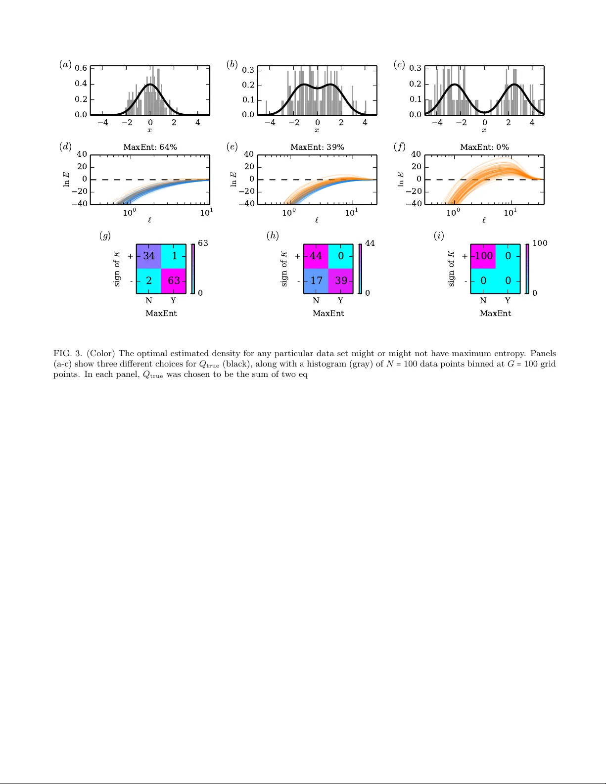
Unification of field theory and maximum entropy methods for learning probability densities

Unification of field theory and maxim um en trop y metho ds for learning probabilit y densities Justin B. Kinney ∗ Simons Center for Quantitative Biolo gy, Cold Spring Harb or L ab or atory, Cold Spring Harb or, New Y ork 11724, USA The need to estimate smo oth probability distributions (a.k.a. probability densities) from finite sampled data is ubiquitous in science. Man y approaches to this problem hav e b een described, but none is yet regarded as pro viding a definitive solution. Maximum en tropy estimation and Ba yesian field theory are tw o such approaches. Both hav e origins in statistical physics, but the relationship b et ween them has remained unclear. Here I unify these tw o metho ds by sho wing that every maximum entrop y density estimate can be recov ered in the infinite smo othness limit of an appropriate Bay esian field theory . I also show that Bay esian field theory estimation can b e p erformed without imp osing any boundary conditions on candidate densities, and that the infinite smo othness limit of these theories reco vers the most common types of maximum entrop y estimates. Ba yesian field theory th us provides a natural test of the maximum entrop y null hypothesis and, furthermore, returns an alternative (low er entrop y) density estimate when the maximum entrop y h yp othesis is falsified. The computations necessary for this approach can b e p erformed rapidly for one-dimensional data, and softw are for doing this is provided. P A CS n umbers: 02.50.-r, 89.70.Cf, 02.60.-x, 11.10.Lm I. INTR ODUCTION Researc h in nearly all fields of science routinely calls for the estimation of smo oth probabilit y densities from finite sampled data [1, 2]. Indeed, the presence of histograms in a large fraction of the scientific literature attests to this need. But the problem of ho w to go b eyond a histogram and recov er a smo oth probability distribution has yet to find a definitive solution, ev en in one dimension. The reader might find this state of affairs surprising. Man y different metho ds for estimating smooth probabil- it y densities are w ell kno wn and commonly used. One of the most p opular metho ds is kernel densit y estimation [1, 2]. Kernel density estimation is easy to carry out, but this approach has little theoretical justification and there is no consensus on certain basic asp ects of its use, suc h as ho w to choose a kernel width or how to treat data p oin ts near a b oundary [3]. Bay esian inference of a Gaussian mixture mo del is another common metho d. This approach, how ever, requires that one assume an ex- plicit functional form of the density that one wishes to learn. Concepts from statistical physics hav e giv en rise to tw o alternativ e approac hes to the density estimation prob- lem: maximum entrop y (MaxEnt) [4, 5] and Bay esian field theory [6 – 14]. Eac h of these approaches has a firm but distinct theoretical basis. MaxEnt derives from the principle of maxim um entrop y as describ ed by Jaynes in 1957 [4]. Ba yesian field theory , which is also referred to as “information field theory” in some of the literature [9], instead uses the standard metho ds of Ba yesian infer- ence together with priors that weigh t p ossible densities according to an explicit measure of smo othness without ∗ Email corresp ondence to jkinney@cshl.edu requiring a particular functional form. P erhaps b ecause the principles underlying these t wo metho ds are differen t, the relationship b et ween these approac hes has remained unclear. MaxEn t density estimation is carried out as follows. One first uses s ampled data to estimate v alues for a c hosen set of momen ts, e.g., mean and v ariance. T yp- ically , all momen ts up to some sp ecified order are se- lected [5, 15]. The probability density that matches these momen ts while ha ving the maxim um p ossible entrop y is then adopted as one’s estimate. All other information in the data is discarded. One can therefore think of the MaxEn t estimate as a n ull hypothesis reflecting the as- sumption that there is no useful information in the data b ey ond the v alues of the sp ecified momen ts [16]. In the Bay esian field theory approach, one first defines a prior on the space of contin uous probability densities. This prior is form ulated using a scalar field theory that fa- v ors smo oth probability densities ov er rugged ones. The data are then used to compute a Bay esian p osterior, and from this one identifies the maxim um a p osteriori (MAP) densit y estimate. Simple field theory priors require that one assume an explicit smo othness length scale ` . How- ev er, an optimal v alue for ` can b e learned from the data in a natural w ay if one instead adopts a prior formed from a scale-free mixture of these simple field theories [6–8]. Scale-free Ba yesian field theories th us provide a w ay to estimate probability densities without having to sp ecify an y tunable parameters. One problem with the field theory priors that ha ve b een considered for this purp ose th us far [6 – 8] is that they imp ose b oundary conditions on candidate densities. This assumption of b oundary conditions is standard practice in physics; it greatly aids analytic calculations and is of- ten w ell-motiv ated b y ph ysical reasoning. In the density estimation con text, ho wev er, such b oundary conditions limit the t yp es of data sets for whic h suc h field theory 2 priors w ould b e appropriate. MaxEnt, by con trast, do es not imp ose any b oundary conditions on the densit y esti- mates it provides. Here I desc ribe a class of Bay esian field theory priors that hav e no b oundary conditions. These priors yield MAP density estimates that exactly match the first few momen ts of the data. In the ` → ∞ limit, suc h MAP esti- mates become iden tical to MaxEn t estimates constrained b y these same momen ts. More generally , I show that a MaxEn t densit y estimate matched to an y momen ts of the data can b e recov ered from Bay esian field theory in the infinite smo othness limit; one need only c ho ose a field theory prior that defines “smoothness” appropriately . This unification of Bay esian field theory and MaxEnt densit y estimation further suggests a natural wa y to test the v alidit y of the MaxEn t h yp othesis against one’s data. If Bay esian field theory iden tifies ` = ∞ as b eing optimal for one’s data set, the MaxEn t h yp othesis is v alidated. If instead the optimal ` is finite, the MaxEn t h yp othesis is rejected in fa vor of a nonparametric density estimate that matches the same moments of the data but has low er en tropy . This pap er is structured as follows. Section I I describ es the deriv ation of an action, S ` , that go verns the p osterior probabilit y of densities under a sp ecific class of Bay esian field theories. Section I II describ es how the MAP den- sit y , which minimizes this action, can b e uniquely derived without assuming any b oundary conditions. A differen- tial op erator I call the “bilateral Laplacian” plays a cen- tral role in eliminating these b oundary conditions. Section IV sho ws that such MAP densit y estimates re- duce to MaxEn t estimates in the ` → ∞ limit. Section V derives an expression for a quantit y , the “evidence ra- tio” E ( ` ) , that allows one to select the optimal v alue for ` given the data. The large ` b ehavior of this evidence ratio is shown to b e characterized by a “ K co efficien t,” the sign of whic h provides a no vel analytic test of the MaxEn t assumption. Section VI formalizes a discrete-space represen tation of this Bay esian field theory inference pro cedure. In ad- dition to being essential for the computational implemen- tation of this method, this discrete representation greatly clarifies wh y no boundary conditions are required to de- riv e the MAP density when one makes use of the bilat- eral Laplacian. Section VI I describes how to compute the MAP densit y (to a sp ecified precision) at all length scales ` . Section VI II illustrates this density estimation approac h on sim ulated data sets. A summary and dis- cussion are provided in section IX. Detailed deriv ations of v arious results from sections I I through VI are provided in App endices A-D. Ap- p endix E presents details of a predictor-corrector homo- top y algorithm that allows the density estimation c om- putations describ ed in this pap er to b e carried out. An op en source softw are implementation of this algorithm for one-dimensional density estimation is provided [17]. Finally , App endix F giv es an expanded discussion of how Ba yesian field theory relates to earlier work in statistics on “maxim um p enalized lik eliho o d” [3, 18, 19]. I I. BA YESIAN FIELD THEOR Y The main results of this pap er are elab orated in the con text of one-dimensional densit y estimation. Many of our results are readily extended to higher dimensions, ho wev er, at least in principle. This issue is discussed in more detail later on. Supp ose we are giv en N data p oints x 1 , x 2 , . . . , x N sampled from a smo oth probabilit y densit y Q true ( x ) that is confined to an interv al of length L . Our goal is to estimate Q true from these data. F ollowing [8], w e first represen t eac h candidate density Q ( x ) in terms of a real field φ ( x ) via Q ( x ) = e − φ ( x ) ∫ dx ′ e − φ ( x ′ ) . (1) This parametrization ensures that Q is p ositiv e and nor- malized [20]. Next w e adopt a field theory prior on φ . Sp ecifically we consider priors of the form p ( φ  ` ) = e − S 0 ` [ φ ] Z 0 ` (2) where S 0 ` [ φ ] =  dx L ` 2 α 2 ( ∂ α φ ) 2 , (3) is the “action” corresp onding to this prior and Z 0 ` =  D φ e − S 0 ` [ φ ] (4) is the asso ciated partition function. The real parame- ter ` is a length scale b elow which fluctuations in φ are strongly damp ed. The parameter α , on the other hand, reflects a fundamental choice in how we define “smo oth- ness.” In this paper w e consider arbitrary positive in- teger v alues of α , for reasons that will become clear. Note, how ever, that previous work has explored the con- sequences of using non-in teger v alues of α [7]. As shown in Appendix A, this c hoice of prior allo ws us to compute an exact p osterior probability p ( φ  data , ` ) o ver candidate densities. W e find that p ( φ  data , ` ) = e − S ` [ φ ] Z ` , (5) where S ` [ φ ] =  dx L  ` 2 α 2 ( ∂ α φ ) 2 + N LRφ + N e − φ  (6) is a nonlinear action, Z ` =  D φ e − S ` [ φ ] (7) is the corresp onding partition function, and R ( x ) = N − 1 N  n = 1 δ ( x − x n ) (8) 3 is the raw data densit y . The deriv ation of Eq. (6) is somewhat subtle. In par- ticular, the action S ` [ φ ] gives a p osterior probability p ( φ  data , ` ) that is not related to p ( φ  ` ) via Bay es’s rule. Ho wev er, upon marginalizing ov er the constant comp o- nen t of φ one finds that p ( Q  data , ` ) is indeed related to p ( Q  ` ) via Bay es’s rule. This latter fact is sufficient to justify the use of Eq. (6) in what follows. See App endix A for details. I II. ELIMINA TING BOUNDAR Y CONDITIONS The MAP field φ ` is defined as the field that mini- mizes the action S ` . T o obtain a differen tial equation for φ ` , previous w ork [6 – 8] imp osed perio dic boundary conditions on φ and used integration by parts to deriv e ` 2 α ( − 1 ) α ∂ 2 α φ ` + N LR − N e − φ ` = 0 . (9) With the p erio dic b oundary conditions in place, this dif- feren tial equation has a unique solution. Ho wev er, im- p osing these b oundary conditions amounts to assuming that Q true ( x ) is the same at both ends of the x -in terv al. It is not hard to imagine data sets for which this assump- tion w ould b e problematic. It is true, of course, that Eq. (9) requires boundary conditions in order to ha ve a unique solution. The reason b oundary conditions are needed is the app earance of the of the standard α -order Laplacian operator, ( − 1 ) α ∂ 2 α . Ho wev er, we assumed b oundary conditions on φ in order to derive Eq. (9) in the first place. It therefore has not b een established that b oundary conditions are required for S ` [ φ ] to hav e a unique minimum. In fact, S ` [ φ ] has a unique minimum without the im- p osition of any b oundary conditions on φ . The b ound- ary conditions on φ assumed in previous work [6 – 8] are therefore unnecessary . Indeed, from Eq. (6) alone we can deriv e a differen tial equation that uniquely sp ecifies the MAP field φ ` . W e start b y rewriting the action as S ` [ φ ] =  dx L  ` 2 α 2 φ ∆ α φ + N LRφ + N e − φ  (10) where the differen tial op erator ∆ α is defined b y the re- quiremen t that ϕ ∆ α φ = ( ∂ α ϕ )( ∂ α φ ) (11) for any tw o fields ϕ and φ . In what follows we refer to ∆ α as the “bilateral Laplacian of order α .” Note that ∆ α is a p ositive semi-definite operator, since  dx φ ∆ α φ =  dx ( ∂ α φ ) 2 ≥ 0 . (12) for ev ery real field φ . W e now pro ve that φ ` is unique by sho wing that S ` [ φ ] is a strictly conv ex function of φ when N > 0. Con- sider the change in S ` [ φ ] up on the p erturbation φ → φ + ψ , where φ and ψ are tw o real fields and  is an in- finitesimal n umber and the field ψ is normalized so that L − 1 ∫ dx ψ 2 = 1. The action will change b y an amoun t S ` [ φ + ψ ] = S ` [ φ ] +   dx ψ δ S δ φ  φ (13) +  2 2  dx  ` 2 α L ψ ∆ α ψ + N L e − φ ψ 2  + ⋯ Because ∆ α is p ositive semi-definite, the O (  2 ) term will b e b ounded from b elow by  2 N exp [ − max ( φ )] and must therefore b e p ositive. The Hessian of S ` is therefore p os- itiv e definite at ev ery φ , establishing the strict conv exity of S ` and th us the uniqueness of φ ` . The requiremen t that δ S `  δ φ = 0 gives the follo wing differen tial equation for φ ` : 0 = ` 2 α ∆ α φ ` + N LR − N e − φ ` . (14) F rom the argument ab o ve w e see that this differential equation, unlike Eq. (9), has a unique solution without the imposition of an y boundary conditions on φ ` . This lac k of a need f or boundary conditions in Eq. (14), despite the need for b oundary conditions in Eq. (9), is due to a fundamental difference b etw een the standard Laplacian and the bilateral Laplacian. This difference o ccurs only at the b oundaries of the x -in terv al. Roughly sp eaking, ∆ α φ is w ell-defined at b oth x min and x max , whereas ( − 1 ) α ∂ 2 α φ is not. This p oin t will b e clarified in Section VI, when we formulate our Bay esian field theory approac h on a finite set of grid p oin ts. In the interior of the x -interv al, how ever, the bilateral Laplacian is identical to the standard Laplacian. T o see this, we integrate Eq. (11) and use in tegration by parts to deriv e  dx ϕ ∆ α φ =  dx ϕ  ( − 1 ) α ∂ 2 α  φ (15) + α − 1  b = 0  ( − 1 ) b ( ∂ α − b − 1 ϕ )( ∂ α + b φ )  x max x min . The second term on the right hand side v anishes if the test function ϕ is c hosen so that ∂ b ϕ = 0 at x min and x max for b = 0 , 1 , . . . , α − 1. The v alue of such test functions φ within the interior of the in terv al are unconstrained, and so ∆ α φ ( x ) = ( − 1 ) α ∂ 2 α φ ( x ) , for all x min < x < x max . (16) IV. CONNECTION TO MAXIMUM ENTR OPY F rom its definition in Eq. (11), w e see that the bi- lateral Laplacian is symmetric and real. This op erator is therefore Hermitian and p ossesses a complete set of orthonormal eigen vectors with corresp onding real eigen- v alues. See App endix B for a discussion of the sp ectrum of the bilateral Laplacian. 4 The k ernel of ∆ α is particularly relev an t to the densit y estimation problem. A field φ is in the k ernel of ∆ α if and only if  dx φ ∆ α φ =  dx ( ∂ α φ ) 2 = 0 . (17) F rom this we see that the kernel of ∆ α is equal to the space of p olynomials of order α − 1. In particular, φ = 1 is in the kernel of ∆ α for all p ositiv e in tegers α . As a result, multiplying Eq. (14) on the left b y unit y and integrating gives ∫ dx e − φ ` = L . The MAP densit y Q ` , which is defined in terms of φ ` b y Eq. (1), is thereb y seen to hav e the simplified form, Q ` = e − φ ` L . (18) If w e multiply Eq. (14) on the left by other p olynomials of order α − 1 and in tegrate, w e further find that  dx Q ` x k =  dx R x k , k = 1 , . . . , α − 1 . (19) Therefore, at ev ery length scale ` , the first α − 1 moments of the MAP density Q ` exactly match those of the data. A t ` = ∞ , the MAP field φ ∞ is restricted to the kernel of the bilateral Laplacian. The corresp onding densit y th us has the form Q ∞ ( x ) = 1 L exp  − α − 1  k = 0 a k x k  , (20) where the v alues of the co efficients a k are determined by Eqs. 18 and 19. Q ∞ is therefore iden tical to the MaxEnt densit y that matc hes the first α − 1 moments of the data [5]. A t ` = 0, the kinetic term in Eq. (14) v anishes. As a result, setting δ S 0  δ φ = 0 giv es Q 0 ( x ) = R ( x ) . (21) W e therefore see that the MAP densit y Q 0 is simply the “histogram” of the data, i.e. the normalized sum of delta functions centered at each data p oint. When we form u- late our inference pro cedure on a grid in section VI, w e will see that Q 0 = R indeed b ecomes a b ona fide his- togram with bins defined b y our c hoice of grid. The set of MAP densities Q ` th us forms a one- parameter “MAP curve” in the space of probability den- sities extending from the data histogram at ` = 0 to the MaxEn t densit y at ` = ∞ . Ev ery densit y Q ` along this MAP curv e exactly matc hes the first α − 1 momen ts of the data. More generally , the MaxEn t densit y estimate con- strained to match any set of moments can b e recov ered in the infinite smo othness limit of an appropriate Bay esian field theory . T o see this, consider a MaxEn t estimate Q ME c hosen to satisfy the generalized moment-matc hing criteria  dx Q ME f j =  dx R f j , j = 1 , 2 , . . . , J (22) for some set of user-sp ecified functions f 1 ( x ) , f 2 ( x ) , . . . , f J ( x ) . A Bay esian field theory that recov ers this MaxEn t estimate in the infinite smo othness limit can b e readily constructed b y using a prior defined b y the action S 0 ξ [ φ ] =  dx L ξ 2 φ ∆ φ (23) where ξ is the (p ositive) smo othness parameter and ∆ is a positive semidefinite operator whose kernel is spanned b y the sp ecified functions f 1 , f 2 , . . . , f J together with the constan t function f 0 ( x ) = 1. The p osterior probabilit y on φ will then b e gov erned b y the action S ξ [ φ ] =  dx L  ξ 2 φ ∆ α φ + N LRφ + N e − φ  . (24) F ollowing the same line of reasoning as ab ov e, we find that the MAP density Q ξ , corresp onding to the field φ ξ that minimizes S ξ , will satisfy  dx Q ξ f j =  dx R f j , j = 0 , 1 , . . . , J (25) regardless of the v alue of ξ . In the infinite smo othness limit ( ξ → ∞ ), the MaxEnt density will b e recov ered, i.e. Q ∞ ( x ) = 1 L exp   − J  j = 0 a j f j ( x )   = Q M E ( x ) (26) where the co efficients a 0 , a 1 , . . . , a j are determined by the constrain ts in Eq. (25). V. CHOOSING THE LENGTH SCALE T o determine the optimal v alue for ` , w e compute p ( data  ` ) = ∫ D φ p ( data  φ ) p ( φ  ` ) . This quantit y , com- monly called the “evidence,” forms the basis for Ba yesian mo del selection [6, 7, 21, 22]. F or the problem in hand, the evidence v anishes when α > 1 regardless of the data. The reason for this is that p ( Q  ` ) is an improp er prior; see App endix C. Ho wev er, the evidence ratio E = p ( data  ` ) p ( data  ∞ ) is finite for all ` > 0. Using a Laplace approximation, which is v alid for large N , w e find that E ( ` ) = e S ∞ [ φ ∞ ] − S ` [ φ ` ]     det ker [ e − φ ∞ ] det row [ L 2 α ∆ α ] η − α det [ L 2 α ∆ α + η e − φ ` ] , (27) where η = N ( L  ` ) 2 α . Here the subscripts “ro w” and “k er” indicate restriction to the row space and k ernel of ∆ α , resp ectively; the e − φ ` terms inside the determinants stand for matrices that hav e the v alues e − φ ` ( x ) (for all x s) arra yed along the main diagonal and zeros everywhere else. See App endix C for the deriv ation of Eq. (27). By construction, the evidence ratio E ( ` ) approaches unit y in the large ` limit. Whether this limiting v alue is approac hed from abov e or below is relev ant to the ques- tion of whether ` = ∞ is optimal, and th us whether the 5 MaxEn t hypothesis is consisten t with the data. Using p erturbation theory ab out η = 0 ( ` = ∞ ), w e find that ln E = K η + O ( η 2 ) , (28) where the co efficient K is [23] K =  i > α N v 2 i − z ii 2 λ i +  i > α j ≤ α z 2 ij + v i z ij j 2 λ i ζ j −  i > α j,k ≤ α v i z ij z j kk 2 λ i ζ j ζ k . (29) Here, λ i and ψ i ( x ) ( i = 1 , 2 , . . . ) denote the eigen v alues and eigenfunctions of L 2 α ∆ α and are indexed so that λ i = 0 for i ≤ α . The eigenfunctions are normalized so that ∫ dx L − 1 ψ i ψ j = δ ij , and in the degenerate subspace ( i, j ≤ α ) they are oriented so that ∫ dx Q ∞ ψ i ψ j = δ ij ζ j for some p ositive real num b ers ζ j . The other indexed quan tities are v i = ∫ dx ( Q ∞ − R ) ψ i , z ij = ∫ dx Q ∞ ψ i ψ j , and z ij k = ∫ dx Q ∞ ψ i ψ j ψ k . Eq. (29) provides a plug-in formula that can b e used to assess the v alidity of the MaxEnt hypothesis. If K > 0, there is guaran teed to b e a finite v alue of ` that has a larger evidence ratio than ` = ∞ . In this case the MaxEnt estimate is guaranteed to b e non-optimal. On the other hand, if K < 0, then ` = ∞ is a lo cal optim um that ma y or may not b e a global optimum as well. Numerical computation of E ov er all v alues of ` is thus needed to resolv e whether the MaxEn t h yp othesis pro vides the b est explanation of the data in hand. VI. DISCRETE SP ACE REPRESENT A TION In this section we retrace the entire analysis ab ov e in the discrete representation, i.e., where the contin u- ous x -interv al is replaced by an evenly spaced set of G grid points. This discrete representation is necessary for the computational implementation of our field theoretic densit y estimation metho d. Happily , our main findings ab o v e are seen to hold exactly up on discretization. This discrete representation also sheds light on how the bilat- eral Laplacian differs from the standard Laplacian and wh y this difference eliminates the need for boundary con- ditions. W e consider G grid p oints ev enly spaced through- out the interv al [ x min , x max ] . Specifically , we place grid p oin ts at x i = x min + h  n − 1 2  , n = 1 , 2 , . . . G (30) where h = L  G is the grid spacing. In mo ving to this discrete representation, functions of x become G - dimensional vectors with elements denoted b y the sub- script n . F or instance, the field φ ( x ) becomes a vector with elemen ts φ n . In tegrals become sums, i.e.,  dx f ( x ) → h G  n = 1 f n , (31) and path in tegrals ov er φ b ecome G -dimensional integrals o ver the elemen ts φ n , i.e.,  D φ →  ∞ −∞ dφ 1  ∞ −∞ dφ 2 ⋯  ∞ −∞ dφ G . (32) W e denote differential op erators in this discrete repre- sen tation with a subscript G . The deriv ative op erator, ∂ G , becom es a ( G − 1 ) by G matrix having elements ( ∂ G ) nm = h − 1 ( − δ n,m + δ n + 1 ,m ) . F or instance, setting G = 8 giv es the 7 by 8 matrix, ∂ 8 = 1 h            − 1 1 0 0 0 0 0 0 0 − 1 1 0 0 0 0 0 0 0 − 1 1 0 0 0 0 0 0 0 − 1 1 0 0 0 0 0 0 0 − 1 1 0 0 0 0 0 0 0 − 1 1 0 0 0 0 0 0 0 − 1 1            . (33) Similarly , the standard α -order Laplacian becomes a ( G − 2 α ) by G matrix, giv en by ( − 1 ) α ∂ G − 2 α + 1 ⋯ ∂ G − 1 ∂ G . F or example, choosing α = 3 and G = 8 yields the a 2 by 8 Laplacian matrix − ∂ 6 8 = 1 h 6  − 1 6 − 15 20 − 15 6 − 1 0 0 − 1 6 − 15 20 − 15 6 − 1  . (34) Because 2 α elements are eliminated from the v ector φ ` up on application of the standard Laplacian, the discrete v ersion of Eq. (9) provides only G − 2 α equations for the G unkno wn v alues of φ ` . 2 α additional constrain ts, typ- ically pro vided in the form of b oundary conditions, are th us needed to obtain a unique solution. By con trast, the α -order bilateral Laplacian is rep- resen ted b y the G b y G matrix ∆ α G = ( ∂ α G ) ⊺ ∂ α G , where ∂ α G = ∂ G − α + 1 ⋯ ∂ G − 1 ∂ G . Indeed, again c ho osing α = 3 and G = 8 w e reco ver an 8 by 8 bilateral Laplacian matrix ∆ 3 8 = 1 h 6              1 − 3 3 − 1 0 0 0 0 − 3 10 − 12 6 1 0 0 0 3 − 12 19 − 15 6 1 0 0 − 1 6 − 15 20 − 15 6 − 1 0 0 − 1 6 − 15 20 − 15 6 − 1 0 0 − 1 6 − 15 19 − 12 3 0 0 0 − 1 6 − 12 10 − 3 0 0 0 0 − 1 3 − 3 1              . (35) The middle t wo ro ws of ∆ 3 8 matc h those of − ∂ 6 8 , reflect- ing the equiv alence of bilateral Laplacians and standard Laplacians in the interior of the x -interv al. How ever, ∆ 3 8 con tains six additional ro ws, three at either end. These are sufficient to specify a unique solution for the 8 el- emen ts of the φ ` v ector. More generally , the discrete v ersion of Eq. (14) provides G equations for the G un- kno wn elemen ts of φ ` and is therefore able to sp ecify a unique solution without the imposition of an y boundary conditions. Using the bilateral Laplacian, w e readily define a dis- cretized v ersion of the prior by adopting S 0 ` [ φ ] = ` 2 α 2 G  n,m ∆ α nm φ n φ m . (36) 6 FIG. 1. (Color) Illustration of the predictor-corrector homotopy algorithm. (a) The MAP curve (bro wn) is approximated using finite set of densities { R, Q ` r , ⋯ , Q ` − 2 , Q ` − 1 , Q ` 0 , Q ` 1 , Q ` 2 , . . . , Q ` m , Q ∞ } . First the MAP density at an in termediate length scale ` 0 = L / √ G is computed. A predictor-corrector algorithm is then used to extend the set of MAP densities outw ard to larger and to smaller v alues of ` . These ` v alues are chosen so that neighboring MAP densities lie within a geo desic distance of ≲  of eac h other. (b) Eac h step Q ` t ′ → Q ` t has tw o parts. First, a predictor step (magenta) computes a new length scale ` t and an appro ximation Q ( 0 ) ` t of Q ` t . A series of corrector steps Q ( 0 ) ` t → Q ( 1 ) ` t → Q ( 2 ) ` t ⋯ (orange) then conv erges to Q ` t . This leads to the posterior action S ` [ φ ] =  n,m  ` 2 α 2 G ∆ α nm φ n φ m (37) + N L G R n φ n δ nm + N G e − φ n δ nm  , (38) where R n is v alue of the data histogram at grid point n , i.e., the fraction of data p oin ts discretized to grid p oint n , divided by bin width h . The corresponding equation of motion is ` 2 α  m ∆ α nm φ `m + N LR n − N e − φ `n = 0 . (39) The kernel of ∆ α G is spanned b y vectors φ ha ving the p oly- nomial form φ n = ∑ α − 1 b = 0 a b x b n . The analogous momen t- matc hing b ehavior therefore holds exactly in the discrete represen tation, i.e., h G  n = 1 Q `n x k n = h G  n = 1 R n x k n (40) where Q ` is related to φ ` via Eq. (18). In the ` → ∞ limit, the MAP density Q ∞ again has the analogous form Q ∞ n = 1 L exp  − α − 1  k = 0 a k x k n  (41) where the co efficien ts a k are chosen to satisfy Eq. (40). Th us, the connection to the MaxEn t density estimate remains in tact up on discretization. The deriv ation of the evidence ratio in Eq. (27) follo ws through without mo dification. The only change is that the functional determinants now b ecome determinan ts of finite-dimensional matrices. The deriv ation of the K co efficien t in Eq. (29) also follows in a similar manner; the only c hange to Eq. (29) is that the the index i now ranges from 1 to G , not 1 to ∞ . VI I. COMPUTING DENSITY ESTIMA TES T o compute density estimates using this field the- ory approac h, we work in the discrete representation describ ed in the previous section. First the user sp ecifies the n umber of grid points G as well as a b ounding b o x [ x min , x max ] for the data. MAP den- sities Q ` are then computed at a finite set of length scales { 0 , ` r , ⋯ , ` − 2 , ` − 1 , ` 0 , ` 1 , ` 2 , ⋯ , ` m , ∞ } , as illustrated in Fig. 1a. This “string of b eads” approximation to the MAP curv e allows us to ev aluate the evidence ratio E o ver all length scales and, to finite precision, iden tify the length scale ` ∗ that maximizes E . This approximation of the MAP curve is computed using a predictor-corrector homotopy algorithm [25]. An o verview of this algorithm is now giv en. Please refer to App endix E for algorithm details. I note that this algo- rithm pro vides more transparen t precision b ounds on the computed Q ` densities than do es the previously reported algorithm of [8]. First, an in termediate length scale ` 0 is c hosen and the corresp onding MAP densit y Q ` 0 is computed. This densit y , Q ` 0 , serves as the starting p oin t from which to trace MAP curve to wards both larger and smaller length scales (Fig. 1a). The algorithm then proceeds in b oth directions, stepping from length scale to length scale and up dating the MAP densit y at each step. During each step, the subsequen t length scale is cho- sen so that the corresponding MAP densit y is sufficien tly similar to the MAP densit y at the preceding length scale. Sp ecifically , in stepping from ` t ′ to ` t , the algorithm c ho oses ` t so that the geo desic distance D geo (see [8, 26]) b et w een Q ` t ′ and Q ` t matc hes a user-sp ecified tolerance  , i.e., D geo [ Q ` t , Q ` t ′ ] ≡ 2 cos − 1   dx  Q ` t Q ` t ′  ≲ . (42) The v alue  = 10 − 2 w as used for the computations de- 7 10 8 6 4 2 0 2 4 x 0.0 0.1 0.2 0.3 ( a ) 10 8 6 4 2 0 2 4 x 0 1 0 − 1 1 0 0 1 0 1 ∞ ` ( b ) 0.0 0.1 0.2 1 0 - 1 1 0 0 1 0 1 ` 15 10 5 0 5 10 15 l n E ( c ) 1 0 - 1 1 0 0 1 0 1 ` 2.4 2.6 2.8 3.0 3.2 3.4 3.6 H ( b i t s ) ( d ) FIG. 2. (Color) Density estimation without b oundary con- ditions using the α = 3 field theory prior. (a) N = 100 data p oin ts w ere drawn from a simulated densit y Q true (blac k) and binned at G = 100 grid points. The resulting histogram (gra y) is shown along with the field theory density estimate Q ` ∗ (or- ange) and the corresp onding MaxEn t estimate Q ∞ (blue). (b) The heat map shows the densities Q ` in terp olating b etw een the MaxEnt densit y at ` = ∞ and the data histogram at ` = 0. (c) The log evidence ratio E is sho wn as a function of ` . (d) The differential en tropy H = − ∫ dx Q ` ln Q ` [24] is shown as a function of ` ; the entrop y at ` = ∞ is indicated by the dashed line. Dotted lines in (b-d) mark the optimal length scale ` ∗ . scrib ed b elow and shown in Figs. 2 and 3. Stepping in the decreasing ` direction is terminated at a length scale ` r suc h that D geo [ Q ` r , R ] <  . Similarly , stepping in the increasing ` direction is terminated at a length scale ` m suc h that D geo [ Q ` m , Q ∞ ] <  ; the MaxEnt density Q ∞ is computed at the start of the algorithm essentially as describ ed by Ormoneit and White [15]. Eac h step along the MAP curv e is accomplished in tw o parts (Fig. 1b). Given the MAP density Q ` t ′ at length scale ` t ′ , a “predictor step” is used to compute b oth the next length scale ` t as w ell as an approximation Q ( 0 ) ` t to the corresp onding MAP densit y Q ` t . The repeated application of a “corrector step” is then used to compute a series of densities Q ( 1 ) ` t , Q ( 2 ) ` t , . . . that con verges to Q ` t . If the numerics are prop erly implemented, this predictor-corrector algorithm is guaran teed to iden tify the correct MAP densit y Q ` at each of the chosen length scales ` . This is because the action S ` [ φ ] is strictly con- v ex in φ and therefore has a unique minimum (as was sho wn in section I II). The distance criteria in Eq. (42) further ensures that the stepping procedure does not drastically ov erstep ` ∗ . It is also worth noting that, b e- cause ∆ α G is sparse, these predictor and corrector steps can b e sp ed up by using numerical sparse matrix meth- o ds. VI II. EXAMPLE ANAL YSES Fig. 2 provides an illustrated example of this density estimation procedure in action. Starting from a set of sampled data (Fig. 2a, gra y), the homotopy algorithm computes the MAP density Q ` at a set of length scales spanning the interv al ` ∈ [ 0 , ∞ ] (Fig. 2b). The evidence ratio E is then computed at each of these chosen length scales using Eq. (27), and the length scale ` ∗ that max- imizes E is identified (Fig. 2c). Q ` ∗ is then rep orted as the b est estimate of the underlying densit y (Fig. 2a, or- ange). If one further wishes to report “error bars” on this estimate, other plausible densities Q can b e dra wn from the p osterior p ( Q  data ) as describ ed in [8]. The optimal length scale ` ∗ ma y or may not b e infinite. If ` ∗ = ∞ , then Q ` ∗ is the MaxEnt estimate that matches the first α − 1 momen ts of the data. On the other hand, if ` ∗ is finite as in Fig. 2, then Q ` ∗ will hav e lo wer entrop y than the MaxEnt estimate (Fig. 2d) while still exactly matc hing the first α − 1 moments of the data. This re- duced entrop y reflects the use of addition information in the data b eyond the first α − 1 momen ts. It should b e noted that ` ∗ is never zero due to a v anishing Occam factor in this limit. The densit y estimation pro cedure prop osed in this pa- p er thus provides an automatic test of the MaxEnt hy- p othesis. It can therefore b e used to test whether Q true has a hypothesized functional form. F or example, us- ing α = 3 we can test whether our data w as drawn from a Gaussian distribution. This is demonstrated in Fig. 3. In these tests, when data w as indeed dra wn from a Gaus- 8 4 2 0 2 4 x 0.0 0.2 0.4 0.6 ( a ) 1 0 0 1 0 1 ` 40 20 0 20 40 l n E ( d ) MaxEnt: 64% N Y MaxEnt + - s i g n o f K 34 1 2 63 ( g ) 0 63 4 2 0 2 4 x 0.0 0.1 0.2 0.3 ( b ) 1 0 0 1 0 1 ` 40 20 0 20 40 l n E ( e ) MaxEnt: 39% N Y MaxEnt + - s i g n o f K 44 0 17 39 ( h ) 0 44 4 2 0 2 4 x 0.0 0.1 0.2 0.3 ( c ) 1 0 0 1 0 1 ` 40 20 0 20 40 l n E ( f ) MaxEnt: 0% N Y MaxEnt + - s i g n o f K 100 0 0 0 ( i ) 0 100 FIG. 3. (Color) The optimal estimated density for any particular data set might or might not hav e maximum entrop y . Panels (a-c) show three differen t choices for Q true (blac k), along with a histogram (gray) of N = 100 data p oints binned at G = 100 grid p oin ts. In eac h panel, Q true w as chosen to b e the sum of tw o equally weigh ted normal distributions separated by a distance of (a) 0, (b) 2.5, or (c) 5. P anels (d-f ) sho w the evidence ratio curves computed for 100 data sets resp ectiv ely drawn from the Q true densities in (a-c). Blue curves indicate ` ∗ = ∞ ; orange curves indicate finite ` ∗ . Titles in (d-f ) give the p ercen tage of data sets for which ` ∗ = ∞ was found. The heat maps shown in panels (g-i) report the num b er of simulated data sets for which the K coefficient w as p ositive or negative and for which the MaxEnt density w as or was not recov ered. sian density , ` ∗ = ∞ was obtained ab out 64% of the time (Fig. 3a and 3d). By contrast, when data was dra wn from a mixture of t wo Gaussians, the fraction of data sets yielding ` ∗ = ∞ decreased sharply as the separation b et w een the tw o Gaussians was increased (Figs. 3b, 3c, 3e, and 3f ). In a similar manner, this density estimation approac h can b e used to test other functional forms for Q true , either by using the bilateral Laplacian of differ- en t order α , or by replacing the bilateral Laplacian with a differential operator having a kernel spanned b y other functions whose exp ectation v alues one wishes to match to the data. The method used to select ` ∗ b oth here and in pre- vious work [6, 7] is sometimes referred to as “empirical Ba yes”: for ` ∗ w e choose the v alue of ` that maximizes p ( data  ` ) . By contrast, [8] used a fully Ba yesian approac h b y p ositing a Jeffreys prior p ( ` ) then choosing the length scale ` that maximizes p ( data , ` ) ∼ p ( data  ` ) p ( ` ) . It can b e reasonably argued that the empirical Ba yes metho d adopted here is less sensible than the fully Bay esian ap- proac h. How ever, in the fully Ba yesian approach the as- sumed prior p ( ` ) obscures the large ` b eha vior of the evidence ratio E . This large ` b ehavior is nontrivial and p oten tially useful. As shown in section V, the b eha vior of E in the large ` limit is gov erned by the K co efficien t defined in Eq. (29). The sign of the K co efficient can therefore b e used to assess the MaxEn t h yp othesis without ha ving to compute E at every length scale. This suggestion is supp orted b y the sim ulations shown in Fig. 3. Here, the sign of K (p ositive or negative) p erformed well as a proxy for whether the MaxEnt estimate was recov ered (no or yes, resp ectiv ely) from a full computation of the MAP curv e; see Figs. 3g [27], 3h, and 3i. These results suggest that the K co efficien t, for whic h Eq. (29) provides an analytic expression, might allow an exp edien t test of the MaxEnt h yp othesis when computation of the entire MAP curve is less feasible, e.g., in higher dimensions. IX. SUMMAR Y AND DISCUSSION Bialek et al. [6] show ed that probability density esti- mation can b e formulated as a Bay esian inference prob- lem using field theory priors. Among other results, [6] deriv ed the action in Eq. (6) and sho wed how to use a Laplace appro ximation of the evidence to select the op- timal smo othness length scale [28]. Ho wev er, p eriodic 9 b oundary conditions w ere imposed on candidate densi- ties in order to transform the standard Laplacian into a Hermitian op erator. The MaxEn t densit y estimate t ypi- cally violates these b oundary conditions, and as a result the abilit y of Ba yesian field theory to subsume MaxEn t densit y estimation wen t unrecognized in [6] and in follow- up studies [7, 8]. Here w e hav e seen that b oundary conditions on candi- date densities are unnecessary . The bilateral Laplacian, defined in Eq. (11), is a Hermitian op erator that imp oses no b oundary conditions on functions in its domain, yet is equiv alen t to the standard Laplacian in the interior of the interv al of in terest. Using the bilateral Laplacian of v arious orders to define field theory priors, we recov ered standard MaxEn t density estimates in cases where the smo othness length scale was infinite. W e also obtained a nov el criterion for judging the appropriateness of the MaxEn t h yp othesis on individual data sets. More generally , Bay esian field theories can be con- structed for any set of momen t-matching constraints. One need only replace the bilateral Laplacian in the ab o v e equations with a differen tial operator that has a k ernel spanned by the functions whose mean v alues one wishes to match to the data. The resulting field the- ory will subsume the corresponding MaxEn t h yp othesis, and thereb y allow one to judge the v alidity of that h y- p othesis. Analogous approac hes for estimating discrete probabilit y distributions can b e formulated b y replacing in tegrals o ver x with sums ov er states. The elimination of b oundary conditions remov es a con- siderable point of concern with using Ba y esian field the- ory for estimating probability densities. As demonstrated here and in [8], the necessary computations are readily carried out in one dimension. One issue not inv estigated here – the large N assumption used to compute the evi- dence ratio – can likely be addressed by using F eynman diagrams in the manner of [9]. In the author’s opinion, the problem of ho w to choose an appropriate prior appears to b e the primary issue standing in the w ay of a definitive practical solution to the density estimation problem in 1D. It is not hard to imagine different situations that would call for qualita- tiv ely differen t priors, but understanding which situa- tions call for which priors will require further study . The author is optimistic, how ever, that the v ariety of pri- ors needed to address most of the 1D densit y estimation problems t ypically encountered might not be that large. This field theory approac h to densit y estimation read- ily generalizes to higher dimensions – at least in principle. Additional care is required in order to construct field the- ories that do not pro duce ultra violet div ergences [6], and the best wa y to do this remains unclear. The need for a v ery large n umber of grid p oints also presents a substan- tial practical challenge. Grid-free metho ds, such as those used b y [11, 29], may provide a wa y forward. A CKNOWLEDGMENTS I thank Gurinder At wal, Curtis Callan, William Bialek, and Vija y Kumar for helpful discussions. Sup- p ort for this work was provided b y the Simons Cen ter for Quantitativ e Biology at Cold Spring Harb or Lab ora- tory . App endix A: Deriv ation of the action Our deriv ation of the action S ` [ φ ] in Eq. (6) of the main text is essentially that used in [8]. This deriv ation is not en tirely straight-forw ard, how ev er, and the details of it hav e yet to be rep orted. The prior p ( φ  ` ) , which is defined b y the action S 0 ` in Eq. (3), is improper due to the differential op erator ∆ α ha ving an α -dimensional kernel; see section I I I. T o a void unnecessary mathematical difficulties, we can ren- der p ( φ  ` ) prop er by considering a regularized form of the action S 0 ` [ φ ] =  dx L 1 2 φ  ` 2 α ∆ α +   φ, (A1) where  is an infinitesimal p ositiv e num b er. All quantities of interest, of course, should b e ev aluated in the  → 0 limit. The corresponding prior o v er Q is p ( Q  ` ) =  ∞ −∞ dφ c p ( φ  ` ) =  2 π  e − S 0 ` [ φ nc ] Z 0 ` . (A2) Here w e hav e decomp osed the field φ using φ ( x ) = φ nc ( x ) + φ c (A3) where φ c is the constant F ourier comp onent of φ and φ nc ( x ) is the non-constan t component of φ . The lik eli- ho od of Q given the data is given by p ( data  Q ) = N  n = 1 Q ( x n ) . (A4) Using the identit y a − N = N N Γ ( N )  ∞ −∞ du e − N  u + ae − u  , (A5) whic h holds for any p ositive num b ers a and N , we find that the likelihoo d of Q can be expressed as p ( data  Q ) = N N L N Γ ( N )  ∞ −∞ dφ c e − ∫ dx L  N LRφ + N e − φ  . (A6) The prior probabilit y of Q and the data together is there- fore giv en by p ( data , Q  ` ) = N N L N Γ ( N )  2 π  1 Z 0 `  ∞ −∞ dφ c e − S ` [ φ ] , (A7) where S ` [ φ ] is the action from Eq. (6). 10 The “evidence” for ` – i.e., the probability of the data giv en ` – is therefore giv en by , p ( data  ` ) = N N L N Γ ( N )  2 π  Z ` Z 0 ` , (A8) where Z ` is the partition function from Eq. (7). The p osterior distribution ov er Q is then given by Bay es’s rule: p ( Q  data , ` ) = p ( data , Q  ` ) p ( data  ` ) (A9) =  ∞ −∞ dφ c e − S ` [ φ ] Z ` . (A10) This motiv ates us to define the p osterior distribution ov er φ as p ( φ  data , ` ) ≡ e − S ` [ φ ] Z ` . (A11) This definition of p ( φ  data , ` ) is consistent with the for- m ula for p ( Q  data , ` ) obtained in Eq. (A10), in that p ( Q  data , ` ) =  ∞ −∞ dφ c p ( φ  data , ` ) . (A12) Ho wev er, Eq. (A11) violates Bay es’s rule, since p ( φ  data , ` ) ≠ p ( data , φ  ` ) p ( data  ` ) . (A13) This is not a problem, how ever, since φ itself is not di- rectly observ able; only Q is observ able. Put another w ay , Eq. (A11) violates Ba yes’s rule only in the w ay that it sp ecifies the b ehavior of φ c . This constant comp onent of φ , ho wev er, has no effect on Q . Note that all of the ab ov e calculations hav e b een ex- act; no large N appro ximation was used. This con trasts with prior w ork [6, 7], which used a large N Laplace ap- pro ximation to deriv e the form ula for S ` [ φ ] . Also note that the regularization parameter  has v anished in the form ulas for the p osterior distributions p ( Q  data , ` ) and p ( φ  data , ` ) . How ever, this parameter still app ears in the form ula for the evidence p ( data  ` ) , b oth explicitly and implicitly through the v alue of Z 0 ` . App endix B: Sp ectrum of the bilateral Laplacian In the contin uum limit, ∆ α = ( ∂ α ) ⊺ ∂ α remains man- ifestly Hermitian and therefore p ossesses a complete or- thonormal basis of eigenfunctions. W e now consider the sp ectrum of this op erator. In what follo ws we will make use the k et notion of quantum mechanics, primarily as a notational con venience. F or any tw o functions f and g and an y Hermitian op erator H , w e define  f  H  g  =  dx L f ∗ H g . (B1) 0 1 ( x − x m i n ) / L 2 1 0 1 2 ψ k ( a ) k = 1 , 2 , 3 0 1 ( x − x m i n ) / L 2 1 0 1 2 ψ k ( b ) k = 4 , 5 , 6 , 7 1 2 3 4 5 6 7 k 0 1 2 3 4 5 6 λ 1 / 6 k × L / π ( c ) FIG. 4. Sp ectrum of the bilateral Laplacian of order α = 3. (a) The first three Legendre p olynomials provide an orthonormal basis for the k ernel of ∆ 3 . These c hoices for ψ 1 , ψ 2 , and ψ 3 are plotted with decreasing opacity . (b) All other eigenfunc- tions are nontrivial linear combinations of factors of the form exp ( iκx ) . This behavior is illustrated b y the basis functions ψ 4 , ψ 5 , ψ 6 , and ψ 7 , whic h are shown in decreasing opacity . (c) The rank-ordered eigen v alues of ∆ 3 lie at or below those of the standard Laplacian with any choice of boundary con- ditions. Shown are the eigen v alues of ∆ 3 (blac k squares), together with the eigen v alues of − ∂ 6 with p erio dic, Dirichlet, or Neumann b oundary conditions (dark, medium, and light gra y circles resp ectively). Note th e con ven tion of dividing b y L in the inner product in tegral. This allows us to tak e inner pro ducts without altering units. F rom  φ  ∆ α  φ  =  dx L  ∂ α φ  2 ≥ 0 , (B2) w e see that ∆ α is p ositive semi-definite. Equality in Eq. (B2) obtains if and only if φ is a p olynomial of order α − 1; suc h p olynomials therefore comprise the null space of ∆ α . More generally , any solution to the eigen v alue equation ∆ α ψ = λψ implies that λ  φ  ψ  =  φ  ∆ α  ψ  for an y test function φ . In tegrating this b y parts gives λ  x max x min dx φ ∗ ψ = α − 1  b = 0  ( − 1 ) b ( ∂ α − b − 1 φ ∗ )( ∂ α + b ψ )  x max x min (B3) + ( − 1 ) α  x max x min dx φ ∗ ∂ 2 α ψ . (B4) Considering test functions φ ( x ) who’s first α − 1 deriv a- tiv es all v anish at the boundary , w e see that in the bulk 11 of the interv al, x min < x < x max , λψ = ( − 1 ) α ∂ 2 α ψ . (B5) An y function of ∆ α m ust therefore b e an eigenfunction of the standard α -order Laplacian, ( − 1 ) α ∂ 2 α , as well. Moreo ver, all boundary terms in Eq. (B4) must v anish b ecause the v alues of φ and its deriv atives at the b ound- ary are indep endent of its integral with any function in the interior. The eigenfunction ψ m ust therefore ha ve the boundary b eha vior 0 = ∂ α + b ψ  x min = ∂ α + b ψ  x max for 0 ≤ b < α. (B6) Note in particular that this b eha vior is exhibited b y poly- nomials of order α − 1, whic h comprise the k ernel of ∆ α . On the other hand, if λ > 0, the corresp onding eigen- function ψ will consist of 2 α terms of the form exp [ iκx ] , where κ = λ 1  2 α e iπ b  α for b = 0 , 1 , . . . , 2 α − 1. The co- efficien ts of these terms will b e such that the b oundary b eha vior in Eq. (B6) is satisfied. T ypically such eigen- functions will not be purely sin usoidal or purely expo- nen tial, but rather will exhibit a non trivial combination of sin usoidal and exp onen tial b eha vior (see Fig. 4b). It should b e emphasized that the b oundary behavior of the eigenfunctions (Eq. (B6)) is not a boundary condition that all functions φ in the domain of ∆ α m ust satisfy . Sp ecifically , although any well-behav ed function φ can b e expressed in the eigenbasis via φ = ∞  k = 0 c k ψ k (B7) for some set of co efficients c k , one will t ypically find that ∂ b φ ≠ ∞  k = 0 c k ∂ b ψ k (B8) b ecause the sum on the right hand side of Eq. (B8) will not b e w ell-defined. The reason for this is that the con- v ergence criterion for Eq. (B7) is weak er than that of Eq. (B8), due to the fact that ψ k ∼ 1 whereas ∂ b ψ k ∼ k b . Therefore, ev en though the right hand side of Eq. (B7) will conv erge for an y particular φ , the right and side of Eq. (B8) typically will not. The ordered eigen v alues of the bilateral Laplacian pro- vide a lo w er bound for the eigenv alues of the standard Laplacian with any set of b oundary conditions. T o see this, note that we can define a p ositiv e semi-definite Her- mitian op erator H bc whose kernel is spanned by all func- tions satisfying a set of s pecified boundary conditions. Let us denote the standard Laplacian with these b ound- ary conditions as ∆ α bc . Then w e can express ∆ bc in terms of the bilateral Laplacian as ∆ α bc = lim A → ∞ ∆ α A (B9) where ∆ α A = ∆ α + AH bc . (B10) In the A → ∞ limit, a prior defined using ∆ α A in place of ∆ α will restrict candidate fields φ to those that satisfy the boundary condition specified by H bc . F rom first-order p erturbation theory , w e kno w that the k ’th eigenv alue of ∆ α A + dA is related to that of ∆ α A b y λ A + dA k = λ A k + dA  ψ A  H bc  ψ A  . (B11) Therefore, the k ’th eigen v alue of ∆ bc is giv en by λ bc k = λ k +  ∞ 0 dA  ψ A k  H bc  ψ A k  (B12) where ψ A k is the (appropriately defined) k ’th eigen vector of the op erator ∆ α A . Because H bc is p ositive semi-definite, the in tegral on the right hand side is greater or equal to zero. W e therefore see that λ bc k ≥ λ k for all k , regardless of what the actual boundary conditions are. This p oin t is illustrated in Fig. 4c, which plots the ordered eigenv alues for the α = 3 bilateral Laplacian to- gether with the ordered eigen v alues of the standard α - order Laplacian with three different types of b oundary conditions: perio dic b oundary conditions, ∂ b ψ  x min = ∂ b ψ  x max , b = 0 , 1 , . . . , 2 α − 1; (B13) Diric hlet boundary conditions, ∂ 2 b ψ  x min = ∂ 2 b ψ  x max = 0 , b = 0 , 1 , . . . , α − 1; (B14) and Neumann b oundary conditions, ∂ 2 b + 1 ψ  x min = ∂ 2 b + 1 ψ  x max = 0 , b = 0 , 1 , . . . , α − 1 . (B15) App endix C: Deriv ation of the evidence ratio W e now turn to the task of ev aluating the partition functions Z ` and Z 0 ` , so that we can compute the evidence p ( data  ` ) using Eq. (A8). Defining Λ = L 2 α ∆ α and η = N ( L  ` ) 2 α and working in the grid represen tation, w e find a Hessian of the form ∂ 2 S ∂ φ m ∂ φ n  φ ` = ` 2 α GL 2 α  Λ mn + δ mn e − φ `n  (C1) The corresp onding Laplace approximation to the path in tegral is therefore given by Z ` ≈ e − S ` [ φ ` ]         ` 2 α 2 π GL 2 α  G det  Λ + η e − φ `         − 1  2 . (C2) Note that the op erator Λ is unitless and has w ell-defined eigen v alues in the G → ∞ limit. Also note that η is unitless. F or these reasons, η will emerge as a natural p erturbation parameter in the ` → ∞ limit. Ev aluating the partition function Z 0 ` requires more care b ecause the regularized form of the action S 0 ` , giv en 12 in Eq. (A1), has to b e used in order for the equations we deriv e to make sense. W e find that Z 0 ` =         ` 2 α 2 π GL 2 α  G det  Λ + η  N         − 1  2 (C3) =         ` 2 α 2 π GL 2 α  G N − α η α  α det row [ Λ ]        − 1  2 . (C4) As in the main text, the subscript “row” on the deter- minan t denotes restriction to the row space of Λ. Note: in mo ving from Eq. (C3) to Eq. (C4), w e ha ve hav e used degenerate perturbation theory in the  → 0 limit. Putting these v alues for Z ` and Z 0 ` bac k into Eq. (A8), w e get p ( data  ` ) =  α − 1 2 √ 2 π N N − α 2 L N Γ ( N ) e − S ` [ φ ` ]     η α det row [ Λ ] det [ Λ + η e − φ ` ] . (C5) Although b oth Z ` and Z 0 ` dep end strongly on the num- b er of grid p oin ts G , the v alue for the evidence do es not. The evidence does, how ever, depend on the regulariza- tion parameter  ; specifically , it is prop ortional to  α − 1 2 . This is the basis for the claim in the main text that the evidence v anishes for α > 1. In the large ` limit, η → 0, and so det  Λ + η e − φ `  → η α det ker  e − φ ∞  det row [ Λ ] (C6) where “ker” denotes restriction to the kernel of Λ. As a result, p ( data  ∞ ) =  α − 1 2 √ 2 π N N − α 2 L N Γ ( N ) e − S ∞ [ φ ∞ ]  det ker [ e − φ ∞ ] . (C7) T aking the ratio of these expressions for p ( data  ` ) and p ( data  ∞ ) , we recov er the formula for the evidence ratio E in Eq. (27). Note that E , unlik e the evidence itself, do es not dep end on the regularization parameter  . App endix D: Deriv ation of the K coefficient The goal of this section is to clarify the large length scale ( ` → ∞ ) b ehavior of ln E = S ∞ [ φ ∞ ] − S ` [ φ ` ] (D1) + 1 2 ln        det ker  e − φ ∞  det row [ Λ ] η − α det [ Λ + η e − φ ` ]        . T o do this w e expand ln E as a p o wer series in η ab out η = 0. W e will find that ln E = K η + O ( η 2 ) where K is a non trivial coefficient, given by Eq. (29), that can be either positive or negativ e dep ending on the data. W e carry out this expansion in three steps: 1. Expand φ ` to first order in η . 2. Expand S ` [ φ ` ] to first order in η . 3. Expand ln det [ Λ + η e − φ ` ] to first order in η . In what follo ws we will use the brac ket notation of Ap- p endix B. The eigen v alues λ i and corresp onding eigen- functions ψ i ( x ) of Λ are tak en to satisfy  ψ i  ψ j  = δ ij for all i, j, (D2) λ i = 0 for i ≤ α, (D3) and  ψ i  e − φ ∞  ψ j  = δ ij ζ j for i, j ≤ α (D4) for some p ositiv e n umbers ζ j . W e will also make use of the follo wing indexed quan tities, v i = L  ψ i  Q ∞ − R  =  dx ( Q ∞ − R ) ψ i (D5) z ij = L  ψ i  Q ∞  ψ j  =  dx Q ∞ ψ i ψ j (D6) z ij k = L  ψ i  Q ∞ ψ j  ψ k  =  dx Q ∞ ψ i ψ j ψ k . (D7) 1. Expansion of φ ` to first order in η . W e b egin by represen ting φ ` as a p o wer series in η . Abusing our subscript notation somewhat, we write φ ` = φ ∞ + η φ 1 + η 2 φ 2 + ⋯ . (D8) Plugging this expansion in to the equation of motion, 0 = Λ φ ` + η ( LR − e − φ ` ) , (D9) then collecting terms of equal order in η , we get, 0 = Λ φ ∞ + η  Λ φ 1 + LR − e − φ ∞  + η 2  Λ φ 2 + e − φ ∞ φ 1  + ⋯ (D10) This expansion m ust v anish at each order in η . A t low est order in η w e reco ver Λ φ ∞ = 0, whic h just reflects the restriction of φ ∞ to the kernel of Λ. A t first order in η , 0 = Λ φ 1 + LR − e − φ ∞ , (D11) whic h w e will now pro ceed to inv estigate. T o compute φ 1 , we first write it in terms of the eigen- functions of Λ, i.e., φ 1 ( x ) =  i A i ψ i ( x ) (D12) for appropriate co efficien ts A i . T aking the inner pro duct of Eq. (D11) with  ψ i  , w e get 0 = λ i A i + L  ψ i  R − Q ∞  (D13) = λ i A i − v i . (D14) Since λ i > 0 for i > α , we find that A i = v i λ i , i > α. (D15) 13 As yet we hav e no information ab out the v alues A i for i ≤ α . F or this w e need to consider the second order term in Eq. (D10). Starting from 0 = Λ φ 2 + e − φ ∞ φ 1 (D16) and dotting each side with  ψ j  for j ≤ α , we find that 0 =  ψ j  Λ  φ 2  +  φ i  e − φ ∞  φ 1  (D17) =  i A i  ψ j  e − φ ∞  ψ i  (D18) = A j ζ j +  i > α A i z ij (D19) Applying Eq. (D15), w e th us see that A j = −  i > α v i z ij λ i ζ j , j ≤ α. (D20) This completes our computation of the A i co efficien ts. W e find that φ ` = φ ∞ + η         i > α v i λ i ψ i −  i > α j ≤ α v i z ij λ i ζ j ψ j        + O ( η 2 ) . (D21) 2. Expansion of S ` [ φ ` ] to first order in η . The action S ` [ φ ] can b e expressed as S ` [ φ ] = N  η − 1 2  φ  Λ  φ  + L  φ  R  +  dx L e − φ  . (D22) Using this expression together with the expansion in Eq. (D8), we find that the v alue of the action S ` at its mini- m um φ ` is S ` [ φ ` ] = S ∞ [ φ ∞ ] + N η  1 2  φ 1  Λ  φ 1  + L  φ 1  R − Q ∞  + O ( η 2 ) . (D23) The first inner pro duct term in Eq. (D23) is 1 2  φ 1  Λ  φ 1  = 1 2  i > α v 2 i λ i , (D24) while second is L  φ 1  R − Q ∞  = −  i > α v 2 i λ i . (D25) This giv es the rather simple result, S ` [ φ ` ] − S ∞ [ φ ∞ ] = − η  i > α N v 2 i 2 λ i + O ( η 2 ) . (D26) 3. Expansion of ln det [ Λ + η e − φ ` ] to first order in η . W e first outline ho w we will go ab out computing ln det Γ where Γ = Λ + η e − φ ` . Calculating this quantit y requires calculating the eigenv alues of Γ. W e will use γ i and ρ i to denote the eigen v alues and corresp onding orthonormal eigenfunctions of Γ, i.e., Γ ρ i = γ i ρ i . (D27) and  ρ i  ρ j  = δ ij . (D28) Our primary task is to compute each eigen v alue γ i as a p o w er series in η : γ i = λ i + η γ 1 i + η 2 γ 2 i + ⋯ . (D29) This task, as w e will see, also requires computing the eigenfunctions ρ i as pow er series in η : ρ i = ψ i + η ρ 1 i + η 2 ρ 2 i + ⋯ . (D30) As usual, it will help to expand ρ 1 i in the eigenfunctions of Λ. W e write ρ 1 i ( x ) =  j B i j ψ j ( x ) , (D31) and will so on proceed to compute the co efficien ts B i j . Keeping in mind that λ i > 0 for i > α , and λ j = 0 for j ≤ α , w e see that ln det Γ = ln  i γ i (D32) = ln        η α    j ≤ α γ 1 i     i > α λ i         (D33) + η   i > α γ 1 i λ i +  i ≤ α γ 2 i γ 1 i  + O ( η 2 ) . (D34) So while the larger eigen v alues of Γ need only b e com- puted to first order in η , the α low est eigenv alues of Γ m ust actually b e computed to second order in η . Per- forming this second order calculation will require that w e (partially) compute the eigenfunctions ρ i to first or- der in η , i.e. compute (some of ) the co efficien ts B i j in Eq. (D31). Plugging Eq. (D29) and Eq. (D30) into Eq. (D27) and collecting terms by order in η , we get 0 = Γ ρ i − γ i ρ i (D35) = ( Λ + η e − φ ∞ + η 2 e − φ ∞ φ 1 )( ψ i + η ρ 1 i + η 2 ρ 2 i ) − ( λ i + η γ 1 i + η 2 γ 2 i )( ψ i + η ρ 1 i + η 2 ρ 2 i ) + O ( η 3 ) (D36) = ( Λ ψ i − λ i ψ i ) + η  Λ ρ 1 i + e − φ ∞ ψ i − λ i ρ 1 i − γ 1 i ψ i  + η 2  Λ ρ 2 i + e − φ ∞ ρ 1 i − e − φ ∞ φ 1 ψ i − λ i ρ 2 i − γ 1 i ρ 1 i − γ 2 i ψ i  + O ( η 3 ) . (D37) 14 The coefficient of eac h term in this expansion m ust v an- ish. F rom the zeroth order term of Eq. (D37) w e recov er the eigenv alue equation Λ ψ i = λ i ψ i , which we already knew. F rom the first order term w e get 0 = Λ ρ 1 i + e − φ ∞ ψ i − λ i ρ 1 i − γ 1 i ψ i . (D38) Dotting this with  ψ k  and using Eq. (D31) then gives 0 =  ψ k  Λ  ρ 1 i  +  ψ k  e − φ ∞  ψ i  − λ i  ψ k  ρ 1 i  − γ 1 i  ψ k  ψ i  (D39) = ( λ k − λ i ) B i k + z ik − γ 1 i δ ik . (D40) If we set k = i , we reco ver the standard first order correc- tion to the eigen v alues, namely γ 1 i = z ii for all i, (D41) in particular, γ 1 j = ζ j for j ≤ α. (D42) W e also see by insp ection of Eq. (D40) that B i k = − z ik λ k for i ≤ α, k > α . (D43) Moreo ver, from the normalization requiremen t of Eq. (D28), 1 =  ρ i  ρ i  (D44) =  ψ i  ψ i  + 2 η  ψ i  ρ i  + O ( η 2 ) (D45) = 1 + 2 η B i i + O ( η 2 ) , (D46) from whic h we conclude that B i i = 0 for all i. (D47) T urning to the second-order term in Eq. (D37), w e no w consider the requirement 0 = Λ ρ 2 i + e − φ ∞ ρ 1 i − e − φ ∞ φ 1 ψ i − λ i ρ 2 i − γ 1 i ρ 1 i − γ 2 i ψ i . (D48) Cho osing i ≤ α , dotting with  ψ i  , and using the fact that λ i = 0, w e find that 0 =  ψ i  e − φ ∞  ρ 1 i  −  ψ i  e − φ ∞ φ 1  ψ i  − γ 1 i  ψ i  ρ 1 i  − γ 2 i (D49) =  j B i j z ij −  j A j z iij − γ 1 i B i i − γ 2 i (D50) No w consider the first term of Eq. (D50). Because B i i = 0 and z ij = ζ i δ ij for i, j ≤ α , no j ≤ α terms contribute to this sum. The third term also v anishes due to B i i = 0. So for i ≤ α , γ 2 i =  j > α B i j z ij −  j > α A j z iij −  j ≤ α A j z iij (D51) = −  j > α z 2 ij λ j −  j > α v j z iij λ j +  j ≤ α k > α v k z j k z iij λ k ζ j (D52) Ha ving computed γ 1 i for all i and γ 2 i for i ≤ α , we can no w find ln det Γ. Plugging in our results for γ 1 i and γ 2 i and using  j ≤ α ζ j = det ker [ e − φ ∞ ] ,  i > α λ i = det row [ Λ ] , (D53) w e get what we set out to find: ln det Γ = ln  η α det ker [ e − φ ∞ ] det row [ Λ ] + η             i > α z ii λ i −  j > α i ≤ α z 2 ij + v j z iij λ j ζ i +  k > α i,j ≤ α v k z j k z iij λ k ζ i ζ j            + O ( η 2 ) . (D54) 4. Putting it all together Putting toge ther our results from Eq. (D26) and Eq. (D54), w e find that to first order in η , ln E = S ∞ [ φ ∞ ] − S ` [ φ ` ] − 1 2 ln  det Γ η α det ker [ e − φ ∞ ] det row [ Λ ]  (D55) = η  i > α N v 2 i 2 λ i − η 2             i > α z ii λ i −  j > α i ≤ α z 2 ij + v j z iij λ j ζ i +  k > α i,j ≤ α v k z j k z iij λ k ζ i ζ j            (D56) = K η , (D57) where K =  i > α N v 2 i − z ii 2 λ i +  j > α i ≤ α z 2 ij + v j z iij 2 λ j ζ i −  k > α i,j ≤ α v k z j k z iij 2 λ k ζ i ζ j . (D58) The form ula for K in Eq. (29) is obtained b y renaming the indices i, j, k in the second and third terms. App endix E: Predictor-corrector homotopy algorithm 1. Computing the MaxEnt densit y W e saw in the main text that adopting the prior de- fined by the action in Eq. (3) renders φ ∞ a p olynomial of order α − 1, i.e., φ ∞ ( x ) = α − 1  i = 0 a i x i (E1) for some vector of coefficients a = ( a 0 , a 1 , . . . , a α − 1 ) . The problem of computing the MaxEnt density Q ∞ therefore reduces to finding the vector a that minimizes the p os- terior action S ∞ ( a ) = N  dx L  LR α − 1  i = 0 a i x i + exp  − α − 1  i = 0 a i x i  . (E2) F ollowing Ormoneit and White [15], w e solve this opti- mization problem using the Newton-Raphson algorithm with bac ktracking. Starting at a 0 = 0 , w e iterate a n → a n + 1 = a n + γ n δ a n (E3) 15 where the vector δ a n is the solution to α − 1  j = 0 ∂ 2 S ∂ a i ∂ a j  a n δ a n j = − ∂ S ∂ a i  a n (E4) and γ n is some num b er in the interv al ( 0 , 1 ] . F rom Eq. (E2), ∂ S ∂ a i = N µ i − N  dx L x i exp  − α − 1  k = 1 a k x k  , (E5) where µ i = ∫ dx R x i is the i ’th momen t of the data, and ∂ 2 S ∂ a i ∂ a j = N  dx L x i + j exp  − α − 1  k = 1 a k x k  . (E6) The Hessian matrix H , with elements H ij = ∂ 2 S ∂ a i ∂ a j , is p ositiv e definite at all a . This is readily seen from the fact that for an y v ector w , w ⊺ H w = N  dx L   i x i w i  2 e − ∑ k a k x k > 0 . (E7) Eq. (E4) will therefore alwa ys yield a unique solution for δ a n . The scalar γ n is chosen so that the c hange in the ac- tion in each iteration is commensurate with the linear appro ximation. Sp ecifically , γ n is first set to 1. Then, if S ∞ ( a n + γ n δ a n ) − S ∞ ( a n ) < γ n 2 α − 1  i = 0 ∂ S ∂ a i  a n δ a n i (E8) is not satisfied, γ n is reduced b y factors of 1 2 un til Eq. (E8) holds. This “damp ening” of the Newton-Raphson metho d is sufficient to guarantee conv ergence [15, 30]. The algorithm is terminated when the magnitude of the c hange in the action,  S ∞ ( a n + 1 ) − S ∞ ( a n ) , falls below a sp ecified tolerance. 2. Predictor step The predictor step computes a change ` → ` ′ in the length s cale, as well as an approximation to the corre- sp onding change φ ` → φ ` ′ in the MAP field. Specifically , the predictor step returns a scalar δ t and a function ρ ( x ) suc h that, t ′ = t + δ t (E9) and φ ` ′ ( x ) ≈ φ ( 0 ) ` ( x ) = φ ` ( x ) + ρ ( x ) δ t, (E10) where t = ln η is a numerically conv enient reparametriza- tion of ` . T o determine the function ρ , we examine the equation of motion, Eq. (D9), at ` ′ : 0 = Λ φ ` ′ + η ′ ( LR − e − φ ` ′ ) (E11) = Λ ( φ ` + ρδ t ) + η e δ t ( LR − e − ( φ ` + ρδ t ) ) (E12) = Λ φ ` + η ( LR − e − φ ` ) (E13) + δ t  Λ + η e − φ `  ρ + η ( LR − e − φ ` )  + O ( δ t 2 ) . The O ( 1 ) term v anishes due to φ ( n ) satisfying the equa- tion of motion at ` . The O ( δ t ) term must therefore v an- ish as well. W e th us obtain a linear equation,  Λ + η e − φ `  ρ = η ( e − φ ` − LR ) , (E14) whic h can b e numerically solved for ρ . The scalar δ t is then c hosen to satisfy the distance criterion,  2 = D 2 geo ( Q ` , Q ` ′ ) (E15) ≈  dx ( Q ` − Q ` ′ ) 2 Q ` (E16) ≈ ( δ t ) 2  dx Q ` ρ 2 . (E17) W e therefore set δ t = ±   ∫ dx Q ` ρ 2 , (E18) with the sign of δ t chosen according to the direction we wish to trav erse the MAP curve. 3. Corrector step The purpose of the corrector step is to accurately solv e the equation of motion, Eq. (D9), at fixed length scale ` . This step is initially used to compute Q ` 0 at the start- ing length scale ` 0 . It is then employ ed to hone in on the MAP density at each new length scale chosen b y the predictor step of the homotop y algorithm. As with the computation of the MaxEn t density , this corrector step uses the Newton-Raphson algorithm with bac ktracking. Starting from a h yp othesized field φ ( 0 ) (e.g., returned by the predictor step), the iteration φ ( n ) → φ ( n + 1 ) = φ ( n ) + γ n δ φ ( n ) (E19) is p erformed. The function δ φ ( n ) and scalar γ n are chosen so that this iteration con verges to the true field φ ` . T o deriv e the field p erturbation δ φ ( n ) , w e pro visionally set γ n = 1 and plug the ab ov e formula for φ ( n + 1 ) in to the equation of motion, Eq. (D9). Keeping only terms of order δ φ ( n ) or less, we see that the field p erturbation δ φ ( n ) is the solution to the linear equation,  Λ + η e − φ ( n )  δ φ ( n ) = η ( e − φ − LR ) − Λ φ ( n ) , (E20) whic h we solv e numerically . As b efore, γ n is then cho- sen so that so that the action decreases b y an amount commensurate with the linear appro ximation, i.e., S ` [ φ ( n + 1 ) ] − S ` [ φ ( n ) ] < γ n 2  dx δ S ` δ φ ( x )  φ ( n ) δ φ ( n ) . (E21) This iterativ e pro cess is terminated when the magnitude of the change in the action,  S ` [ φ ( n + 1 ) ] − S ` [ φ ( n ) ] , falls b elo w a sp ecified tolerance. 16 App endix F: Maximum penalized lik eliho o d and Ba yesian field theory In statistics there is a class of nonparametric tech- niques for estimating smooth functions called “maximum p enalized lik eliho o d” estimation [3, 18, 19]. The central idea b ehind these metho ds is to maximize the likelihoo d function modified b y a heuristic roughness p enalty . In this con text, Silv erman (1982) prop osed using − S ` [ φ ] , defined in Eq. (6), as the penalized lik eliho o d function for probability densit y estimation [18]. This choice was motiv ated b y the observ ation that, when ` = ∞ , one re- co vers a momen t-matching distribution having a familiar parametric form. This early work by Silverman is there- fore relev an t to the results reported here. Ho wev er, the results rep orted here mo ve beyond [18] in a n umber of critical wa ys. First, the connection with MaxEn t estimation w as not recognized in [18], nor was the fact that the MAP densit y Q ` matc hes the same mo- men ts as Q ∞ ev en at finite v alues of ` . Moreo ver, p erio dic b oundary conditions on Q ` w ere assumed in m uch of the analysis describ ed in [18], and the contradiction b et ween these boundary conditions and the results for ` = ∞ w as not discussed. P erhaps most imp ortan tly , the shortcomings of the maxim um penalized lik eliho o d approach highlight the imp ortance of adopting an explicit Bay esian interpreta- tion. Although the p enalized likelihoo d con text of [18] and later work (see [3]) w as sufficien t to motiv ate the form ula for S ` [ φ ] , it provided no motiv ation for comput- ing the evidence p ( data  ` ) . Without the Bay esian notion of evidence, it is unclear ho w to determine the optimal smo othness length scale ` ∗ without resorting to empiri- cal metho ds, such as cross-v alidation. By contrast, the Ba yesian interpretation in tro duced by Bialek et al. [6] and built upon here transparently motiv ates the compu- tation of p ( data  ` ) , thereby pro viding an explicit criterion for choosing ` ∗ . In particular, this Bay esian interpreta- tion is essen tial for our deriv ation of the K co efficient in Eq. (29) of the main text. [1] B. Silv erman, Density Estimation for Statistics and Data Analysis (Chapman and Hall, 1986). [2] D. W. Scott, Multivariate Density Estimation: The ory, Pr actic e, and Visualization (Wiley , 1992). [3] P . P . B. Eggermont and V. N. LaRiccia, Maximum Pe- nalize d Likeliho o d Estimation: V olume 1: Density Esti- mation (Springer, 2001). [4] E. T. Ja ynes, Phys. Rev. 106 , 620 (1957). [5] L. R. Mead and N. P apanicolaou, J. Math. Ph ys. 25 , 2404 (1984). [6] W. Bialek, C. G. Callan, and S. P . Strong, Phys. Rev. Lett. 77 , 4693 (1996). [7] I. Nemenman and W. Bialek, Phys. Rev. E 65 , 026137 (2002). [8] J. B. Kinney , Ph ys. Rev. E 90 , 011301(R) (2014). [9] T. A. Enßlin, M. F rommert, and F. S. Kitaura, Ph ys. Rev. D 80 , 105005 (2009). [10] J. C. Lemm, Bayesian Field The ory (Johns Hopkins, 2003). [11] T. E. Holy , Ph ys. Rev. Lett. 79 , 3545 (1997). [12] V. P eriwal, Phys. Rev. Lett. 78 , 4671 (1997). [13] T. Aida, Ph ys. Rev. Lett. 83 , 3554 (1999). [14] D. M. Sc hmidt, Phys. Rev. E 61 , 1052 (2000). [15] D. Ormoneit and H. White, Economet. Rev. 18 , 127 (1999). [16] I. J. Go od, Ann. Math. Stat. 34 , 911 (1963). [17] Av ailable at https://github.com/jbkinney/14 maxent . [18] B. W. Silv erman, Ann. Stat. 10 , 795 (1982). [19] C. Gu, Smo othing Spline ANOV A Mo dels , 2nd ed., Springer Series in Statistics (Springer, 2013). [20] In tegrals ov er x are restricted to the interv al of length L . [21] D. J. C. MacKay , “Information theory , inference, and learning algorithms,” (Cam bridge Univ ersity Press, 2003) Chap. 28. [22] V. Balasubramanian, Neural Comput. 9 , 349 (1997). [23] See SM for a deriv ation of Eq. (29). [24] T. M. Cov er and J. A. Thomas, Elements of Information The ory , 2nd ed. (Wiley , 2006). [25] E. L. Allgo wer and K. Georg, Numeric al Continuation Metho ds: A n Intr o duction (Springer, 1990). [26] J. Skilling, AIP Conf. Pro c. 954 , 39 (2007). [27] The one trial rep orted in Fig. 3g for which ` ∗ = ∞ ev en though K > 0 is due to difficulties with the numerics in the ` → ∞ limit. [28] See App endix F for a discussion of earlier related work on the “maximum p enalized likelihoo d” formulation of the density estimation problem and how it relates to the Ba yesian field theory approach. [29] I. J. Go o d and R. A. Gaskins, Biometrik a 58 , 255 (1971). [30] S. Boyd and L. V anden b erghe, Convex optimization (Cam bridge Universit y Press, 2009).