Replication, Communication, and the Population Dynamics of Scientific Discovery

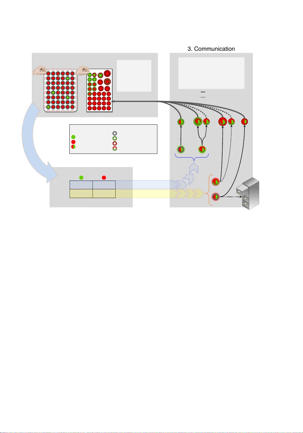
REPLICA TION, COMMUNICA TION, AND THE POPULA TION DYNAMICS OF SCIENTIFIC DISCOVER Y RICHARD MCELREA TH 1,2 AND P AUL E. SMALDINO 1 November 22, 2021 Many published research results are false [1], and controversy continues over the roles of replication and publication policy in improving the reli- ability of research. Addressing these problems is frustrated by the lack of a formal framework that jointly represents hypothesis formation, repli- cation, publication bias, and variation in research quality . W e develop a mathematical model of scientific discovery that combines all of these ele- ments. This model provides both a dynamic model of research as well as a formal framework for reasoning about the normative structure of sci- ence. W e show that replication may serve as a ratchet that gradually sep- arates true hypotheses from false, but the same factors that make initial findings unreliable also make replications unreliable. The most impor- tant factors in improving the reliability of research are the rate of false positives and the base rate of true hypotheses, and we offer suggestions for addressing each. Our results also bring clarity to verbal debates about the communication of research. Surprisingly , publication bias is not al- ways an obstacle, but instead may have positive impacts—suppression of negative novel findings is often beneficial. W e also find that communica- tion of negative replications may aid true discovery even when attempts to replicate have diminished power . The model speaks constructively to ongoing debates about the design and conduct of science, focusing anal- ysis and discussion on precise, internally consistent models, as well as highlighting the importance of population dynamics. Keywords: replication, publication bias, epistemology , scientific method 1 D E PAR T M E N T O F A N T H R O P O L O G Y , U C D A V I S , O N E S H I E L D S A V E N U E , D A V I S C A 9 5 6 1 6 2 C E N T E R F O R P O P U L AT I O N B I O L O G Y , U C D AVI S E-mail address : mcelreath@ucdavis.edu . 1 2 MCELREA TH & SMALDINO I N T R O D U C T I O N Imagine two of your close colleagues have just heard about attempts to replicate their positive resear ch findings. Colleague A is thrilled that the attempt was successful. Colleague B is upset that the attempt was unsuc- cessful. What is the probability that Colleague A ’s hypothesis is true? What is the probability that Colleague B’s hypothesis is false? This is not a fair quiz, because in truth no one knows the answers to these questions. The absence of replication in many fields [2 – 4], combined with the absence of a formal framework for understanding replication, makes it difficult to even outline an answer . In the absence of replication, there is substantial concern that many published findings may be false [1], an argu- ment with empirical support [5 – 7]. The history of science buttresses these observations. A recent catalog of false discoveries of chemical elements out- numbers the current number of real elements in the periodic table [8]. In addition to concerns about replication are concerns about resear ch practice and publication bias. W ithout knowing how many studies wer e conducted but not published, it is not possible to assign evidential value to either ini- tial findings or replications. And it is not yet easy to acquire empirical evi- dence about these factors, as even the best empirical studies of publication bias still rely upon r esear cher self-r eport [3]. Thus many opinions can be sustained about the evidential value of both initial findings and replications. As a result, recent controversies over failed replications demonstrate a lack of consensus on norms for replication and publication [9 – 12]. What is the evidential value of replication, positive or negative? What is the impact of publication bias [13]? If replication is part of an “invisible hand” [14] that corrects scientific errors, how much repli- cation is needed? And what are the risks of poorly designed or interpreted replication attempts [9]? When r eplication is not possible or practical, what other measures can be taken to impr ove the r eliability of r esearch? These questions r emind us that little is understood about the population dynamics of discovery , r eplication, and scientific communication. Much more attention has been given to individual methods of research design and data analysis. And while it is useful to analyze resear ch methods in isola- tion, such calculations are unsatisfying. A lot of resear ch activity is hidden from the public recor d. This means the actual number of findings for an hy- pothesis may never be known [13]. And since researchers select hypotheses for further study from the literature itself, findings and publication biases cascade into other findings, interacting with biases and incentives [15]. T o know the evidential value of resear ch, we must study the popula- tion dynamics that produce it [14, 16 – 18]. So here we construct and solve a mathematical model of scientific beliefs formed by a population of bound- edly rational agents who accumulate evidence for and against hypotheses. THE POPULA TION DYNAMICS OF SCIENTIFIC DISCOVERY 3 W e adopt a general signal detection framework that may apply to diverse statistical paradigms, whether p -valued or Bayesian. W e study the joint dynamics that arise from replication, publication bias, and dif ferences in resear ch quality between original studies and replications. Our goal is not to accurately simulate science, but rather to understand it better using the same reductionist tools that have been so successful in illuminating pop- ulation dynamics more generally [19, 20]. Our model implicitly provides, for example, a neutral model of scientific dynamics in which all hypotheses are false and yet discoveries are continuously published. It also provides a range of “selectionist” models that might be compared to data. The clarity of a quantitative framework will stimulate and clarify the development of later empirical investigation and experimental intervention. The paper proceeds by first outlining the dynamic structure of the model. W e then solve the model for both its long-run dynamics and its epistemo- logical implications—what should a rational agent believe about an hy- pothesis, given a record of published results? W e present a general interpre- tation of the joint dynamics, so the reader can extrapolate lessons from our simple model to the complexity and diversity of real science. W e conclude by relating our results to ongoing debates about improving the reliability of scientific resear ch. M O D E L D E S C R I P T I O N The model is illustrated in Fig. 1. W e have also constructed an interactive, web-based tutorial on the conceptual foundations of the model, as well as fully adjustable simulation code, available at \protect http://xcelab.net/replication/. A population of resear chers studies many differ ent hypotheses. Each hy- pothesis is either true (green) or false (red). These hypotheses could be sim- ple associations, such as green jelly beans cause acne [21], or more general claims, such as evolution is pr edictable . Research r esults in either a positive or a negative finding. These findings may be the result of formal hypothesis tests or informal assessments. T rue hypotheses produce positive findings more often than do false hypotheses, but the r esearchers never know for sure which hypotheses are true. Under these assumptions, the only infor- mation relevant for judging the truth of an hypothesis is its tally , the dif fer - ence between the number of published positive findings and the number of published negative findings for each hypothesis, and we summarize re- sults in terms of these tallies. In reality , much other information is relevant to judging the truth of an hypothesis. Our assumptions are tactical ones. More complex models of scientific communication ar e possible, but any such model must include the components in our model, and so our results establish a critical baseline. 4 MCELREA TH & SMALDINO 1. Hypothesis Selection ! Novel hypotheses ! T ested hypotheses ! A previously tested hypothesis is selected for replication with probability r, otherwise a novel (untested) hypothesis is selected. Novel hypotheses are true with probability b. ! 1 – " r ! r ! 2. Investigation ! T ! Real truth of hypothesis ! Probability of result ! 1 – β α β 1 – α + – 3 . C o mmu n i ca t i o n ! Experimental results are communicated to the scientific community with a probability that depends upon both the experimental result (+, –) and whether the hypothesis was novel (N) or a replication (R). Communicated results join the set of tested hypotheses. Uncommunicated replications revert to their prior status. ! 1 – C N – C N – positive results ! negative results ! 1 – C R+ C R+ New result communicated ! New result not communicated ! 1 – C R– C R– File drawer ! novel ! replic. ! novel ! replic. ! True (T) ! False (T) ! KEY ! Interior = true epistemic state ! Exterior = experimental evidence ! Unknown ! Positive (+) ! Negative (–) ! General case ! General case (+ or –) ! F ! F I G U R E 1 . Population dynamics of replication. Each time interval, resear ch activity has three stages that alter these tal- lies. In stage 1 (Fig. 1, upper-left) each r esearcher chooses to investigate one of n previously published hypotheses, with probability r , or a novel hypothesis, with pr obability 1 − r . When r eplicating, a r esearcher chooses a previously published hypothesis at random and performs a new study of it. Later , we allow resear chers to target hypotheses with specific tally values, rather than choosing at random. A novel hypothesis is true with probability b , the base rate , reflecting mechanisms of hypothesis formation. Untutored intuition, for example, may be expected to yield a very low b . Genome wide association studies likewise have low b , because relatively few loci are as- sociated with any particular phenotype. There is no consensus on base rate, except that most scientists we know believe their own personal b values are better than average. So we allow b to vary freely in the model. In stage 2, a true hypothesis pr oduces a positive finding 1 − β of the time, its power . A false hypothesis produces a positive finding α of the time, its false positive rate . W e assume that 1 − β > α . Later we allow the values of β and α to differ between replication attempts and initial studies. Note that β and α are not merely properties of a statistical procedure, but rather of an THE POPULA TION DYNAMICS OF SCIENTIFIC DISCOVERY 5 entire investigation. For example, using several procedur es and selecting the one that produces a positive r esult will inflate α [22]. In stage 3, findings may be communicated to other resear chers. Not ev- ery finding is communicated, either because no one tries to communicate it or rather because it cannot be published. Only communicated findings can adjust a tally . Let c N − be the probability that a negative ( − ) finding about a new (N) hypothesis is communicated. W e assume for simplicity that all new positive results are communicated ( c N + = 1). Even though replication findings are evidentially equivalent to novel findings, they may be commu- nicated with differ ent probability . Let c R − and c R + be the probabilities that replications with negative and positive findings, respectively , are commu- nicated. These assumptions define the dynamics of the expected numbers of true and false hypotheses with a given tally . W e present the full recursions in the Supporting Material. In the simplest case (full communication: c N − = c R − = c R + = 1), the number n T , s of true hypotheses with an observed tally s in the next time step is given by: n 0 T , s = n T , s + an r  − n T , s n + n T , s − 1 n ( 1 − β ) + n T , s + 1 n β  (1) where a > 0 is the rate of resear ch activity as a proportion of n . This ex- pression says that the number in the next time step is just the current num- ber plus all of the flows in and out caused by replications. In the case that s = − 1 or s = 1, there is an additional term an ( 1 − r ) b β or an ( 1 − r ) b ( 1 − β ) , respectively , to represent the inflow of novel findings. Recursions n 0 F , s for false hypotheses are constructed from a change in variables: 1 − β → α , b → 1 − b . Notice that this implies that the model is easily extended to any number of hypothesis types, such as effect size differences, that differ in power and false-positive rate. W e analyze the true / false dichotomy because of its prominence and simplicity . A N A L Y S I S By literature review , a tally can be constructed for any given hypothe- sis. Given an observed tally , but a number of possibly unobserved studies, what is the probability that an hypothesis is correct? The model allows us to address this question for a diversity of scenarios. Before presenting the solutions, note that the answers that the model provides can be understood both from a pur e population dynamics perspective and from a pr obabilistic reasoning perspective. From the dynamics perspective, the population will converge from any initial condition to a unique steady state in which the so- lutions give fr equencies of true hypotheses at each tally value. Equally valid is the epistemological perspective that the solutions tell us for any unique hypothesis the probability it is true, given a state of information [23]. One 6 MCELREA TH & SMALDINO consequence of this is that the solutions do not requir e that all hypotheses share the same parameter values. For each tally value s , we solved for the steady state proportions of true and false hypotheses, ˆ p T , s and ˆ p F , s . W e also derived the same solutions un- der the probabilistic interpretation, and verified our solutions numerically and through stochastic simulation. W e present complete analytical solu- tions in the Supporting Material. In the simplest case (for full communica- tion), solutions take the form: ˆ p T , s = b ( 1 − r ) ∞ ∑ m = 1 r m − 1  m 1 2 ( m + s )  ( 1 − β ) 1 2 ( m + s ) β 1 2 ( m − s ) (2) This expression defines an infinite geometric series of binomial probabilities arising from all of the differ ent possible histories by which a true hypoth- esis could achieve a tally of s , for every possible number of findings m . In the majority of cases, only the first few terms of the series are important, because of the leading factor r m − 1 . This fact also informs us that the rate of convergence to steady state will be quite rapid, unless r is large. For any particular tally , for example s = 1, expression (2) yields a closed- form solution like: ˆ p T ,1 = b ( 1 − r ) 2 β r 2   1 − 4 r 2 β ( 1 − β )  − 1 2 − 1  (3) For arbitrary communication parameters, the solutions have a similar struc- ture, but are instead a series of multinomial probabilities in which the events are combinations of findings ( + or − ) and communication outcomes. These solutions are not easy to interpret by inspection. But they do pro- vide answers to the question: what is the probability that an hypothesis with a given tally is correct? For any tally s , we can calculate: Pr ( true | s ) = ˆ p T , s ˆ p T , s + ˆ p F , s , Pr ( s | true ) = ˆ p T , s ∑ i ˆ p T , i , Pr ( s | false ) = ˆ p F , s ∑ i ˆ p F , i (4) The pr ecision of a tally s is Pr ( true | s ) , the pr oportion of hypotheses with tally s that are true. The sensitivity , Pr ( s | true ) , is the proportion of true hy- potheses with tally s . It indicates where the true hypotheses are. Sensitivity is important because a high precision for a tally s is little help when there are few hypotheses that achieve a tally s . And the specificity , Pr ( s | false ) , is the proportion of false hypotheses with tally s , indicating where the false hypotheses are. W e use these definitions to explain the behavior of the sys- tem. Overall dynamics. Fig. 2 describes the overall dynamics of precision, as a function of the differ ent parameters. In each panel, the trend lines show the proportion of true hypotheses at each tally on the vertical axis. The tally corresponding to each trend is indicated by a number . The horizontal THE POPULA TION DYNAMICS OF SCIENTIFIC DISCOVERY 7 axis in each panel varies a single parameter . Each vertical hairline shows the value of each parameter that is held constant in other panels. This fig- ure is complex. W e’ll use it to highlight the most important factors in the reliability of findings and demonstrate counter-intuitive aspects of commu- nication. Then in the next section, we’ll turn to a more general explanation of the causes of these results. There are two clusters of plots. The top cluster represents a normatively optimistic scenario, with an auspicious base rate ( b = 0.1), unusually high power (1 − β = 0.8), low false-positive rate ( α = 0.05), and high communi- cation rates. The bottom cluster repr esents a pessimistic, or perhaps more realistic [24, 25], scenario with low base rate ( b = 1/ 1000), lower power (1 − β = 0.6), higher false-positive rate ( α = 0.1), and publication bias re- sulting in low communication of replications and negative findings. The range of base rates we show represents everything from genome wide as- sociation studies, on the low end ( b < 10 − 4 ), to predicting the winner of a presidential election, on the high end ( b = 0.5). Every scientist will have a differ ent opinion about which values r epresent realism. So in the Sup- porting Material, we provide a Mathematica notebook for r eproducing and altering these plots, so the reader can explore alternative scenarios of in- terest. But keep in mind that unrealistic scenarios are just as important for comprehending system dynamics. First, notice that at tally s = 1 very many resear ch findings are false. In the top cluster , the base rate must get quite high before a majority of hy- potheses with tally s = 1 are true. In the bottom cluster , only the highest displayed base rates are sufficient. This dynamically replicates Ioannidis’ direct calculation [1], even in the absence of bias and multiple testing. Many initially published findings ar e false, unless the base rate is high, and with- out any invocation of fraud or resear cher bias. Second, notice that replication helps, but how much it helps varies greatly . In the top cluster , even one positive replication at s = 2 renders most hy- potheses true, at a base rate of b = 0.1. At lower base rates, s = 3 or s = 4 is requir ed to raise precision above one-half. In the bottom cluster , low power and high false-positive rate make replication quite inefficient. Even at high base rates, s = 3 is needed. At low base rates, s = 5 or more is required. In either cluster , achieving near-certainty that an hypothesis is true always requir es replication, even with a base rate as high as b = 0.1. In general, the same factors that make initial findings unreliable also make replications less reliable. Note also that the rate of replication, r in panel (b), has remarkably little impact. This is because replication impacts the rate at which hypotheses reach different tallies, but not so much the pr ecision at each tally . Therefor e 8 MCELREA TH & SMALDINO      0.001 0.1 0.5 0 0.2 0.5 0.8 1 0 0.1 0.3 0.5 0 0.2 0.5 0.8 1 0.5 0.8 0.99 0 0.2 0.5 0.8 1 0.05 0.1 0.15 0.2 0 0.2 0.5 0.8 1 0 0.25 0.5 0.75 1 0 0.2 0.5 0.8 1 0 0.25 0.5 0.75 1 0 0.2 0.5 0.8 1 0 0.25 0.5 0.75 1 0 0.2 0.5 0.8 1      0.001 0.1 0.5 0 0.2 0.5 0.8 1 0 0.1 0.3 0.5 0 0.2 0.5 0.8 1 0.5 0.8 0.99 0 0.2 0.5 0.8 1 0.05 0.1 0.15 0.2 0 0.2 0.5 0.8 1 0 0.25 0.5 0.75 1 0 0.2 0.5 0.8 1 0 0.25 0.5 0.75 1 0 0.2 0.5 0.8 1 0 0.25 0.5 0.75 1 0 0.2 0.5 0.8 1 Proportion true Proportion true 1 3 5 (a) (b) (c) (d) (e) (f) (g) 5 5 5 5 5 5 Proportion true Proportion true base rate ( b ) replication rate ( r ) power (1– β ) false-positive rate ( α ) comm. neg. rep. ( c R– ) comm. pos. rep. ( c R+ ) comm. neg. new ( c N– ) 1 2 3 0 4 (a) (b) (c) (d) (e) (f) (g) 0 1 1 1 1 1 Optimistic scenario Pessimistic scenario 3 3 3 3 3 3 1 0 2 0 0 0 0 base rate ( b ) replication rate ( r ) power (1– β ) false-positive rate ( α ) comm. neg. rep. ( c R– ) comm. pos. rep. ( c R+ ) comm. neg. new ( c N– ) F I G U R E 2 . Effects of base rate, r eplication, power , false-positives, and communication on the probability that an hypothesis with a given tally is true. The two clusters illustrate differ ence scenarios. The blue trends, each labeled with its tally value, show precision as it varies by the parameter on each horizontal axis. The numbers indicate the tally of a curve. Dashed curves are tallies of an even number . The vertical hairlines show the parameter values held constant across panels within the same cluster . at low replication rates, few hypotheses will ever attain s = 5, but those that do are almost certainly tr ue. W e expand on this point in the next section. Third, communication of findings, panels (e-g), can both assist discovery or hinder it. Suppression of negative r eplications (e) r educes pr ecision. But THE POPULA TION DYNAMICS OF SCIENTIFIC DISCOVERY 9 suppression of positive replications (f) and novel negative findings (g) ei- ther improves pr ecision or has almost no impact on it. These aspects of the population dynamics are counter-intuitive, but quite general and revealing. The next section explains them. Dynamics of communication. The “file drawer pr oblem” [13] arises when the failure to publish negative findings distorts the estimated str ength of an association. W e consider a related phenomenon by asking how changes in the communication parameters c N − , c R − , and c R + alter the pr ecision, sensi- tivity , and specificity across tallies. In the pr ocess, we’ll have opportunity to explain the joint dynamics of resear ch quality and communication biases. In this model, it is rarely best to communicate everything. In the Sup- porting Material, we prove for the case of small b (such that b 2 ≈ 0) and small r ( r 3 ≈ 0) that c N − < 1 will improve precision when α < β (usually satisfied), that c R − < 1 improves precision when α > 1 2 (hopefully never satisfied), and that c R + < 1 improves precision whenever β − α ≤ 1 4 (of- ten satisfied). So some suppression of novel negative findings ( c N − < 1) and positive replications ( c R + < 1) can improve the value of replication. At larger b and r , the conditions are more complicated, but the qualitative finding remains intact. T o grasp why suppressing findings might help us learn what is true, think of replication as epistemological chromatography . Chromatography is a set of techniques for separating substances that are mixed together . For example, mixed plant pigments can be separated by painting the mixture onto the tip of a strip of filter paper and then soaking the tip in a solvent. Differ ent pigments bind more or less strongly to the solvent or the paper . Therefor e as the paper absorbs the solvent, different pigments travel at dif- ferent speeds, eventually separating and appearing as differently colored bands on the paper . In the epistemological case, it is true and false hy- potheses that are mixed. W e wish to separate the true ones from the false. Replication applies a “solvent” that diffuses false hypotheses towards neg- ative tallies and tr ue hypotheses towards positive tallies. A true hypothesis diffuses upwar ds with pr obability ( 1 − β ) c R + , while a false hypothesis dif- fuses downwar ds with probability ( 1 − α ) c R − . Thus the communication parameters adjust rates of dif fusion. Just as manipulating rates of chemical diffusion can improve real chromatography , manipulating communication can improve epistemological chr omatography . In Fig. 3, we turn on communication one parameter at a time, in order to explain the contribution of each mode of communication to the r esulting population dynamics. All four panels (a, b, c, d) show steady state preci- sion, sensitivity , and specificity and use b = 0.001, r = 0.2, 1 − β = 0.8, and α = 0.05. These values are chosen for clarity of illustration. In the Sup- porting Material, we pr ovide a Mathematica notebook to construct plots for 10 MCELREA TH & SMALDINO c N– = c R– = c R+ = 1. Tr u e and false hypotheses diffuse in both directions, and everything is communicated. Since most effort investigates new findings at tally –1, few hypotheses ever achieve a high tally , but those that do have high precision . (a) Positive only c N– = 0, c R– = 1, c R+ = 0. T allies can only decrease. False hypotheses diffuse down faster than true ones. But since the mixture at tally +1 is mostly false, precision is always low . (b) Negative only c N– = 0, c R– = 0, c R+ = 1. Only positive findings are initially communicated, and replication can only increase tallies, which are here counts of positive findings. Tr u e hypotheses diffuse upward faster than false ones. So large tallies have a high precision , the proportion of true hypotheses. (c) Screen and check Proportion Solid : c N– = 0, c R– = 1, c R+ = 1. Up diffusion of true hypotheses is aided by down diffusion of false ones from the mixed source tally +1. Compare precision to (a) . Dashed : c N– = 0, c R– = 1, c R+ = 0.2. Suppressing positive replications regulates the rate of up diffusion, purifying high tallies at the price of sensitivity . (d) T otal communication 1– α β 1– β α                            - 5 - 3 - 1 1 3 5 0 0 0.2 0.5 0.8 1 Proportion Proportion Proportion T ally                               0 2 4 6 8 10 0 0 0.2 0.5 0.8 1                                    - 10 - 8 - 6 - 4 - 2 0 0 0 0.2 0.5 0.8 1 1– β α 1– α β                              - 5 - 3 - 1 1 3 5 0 0 0.2 0.5 0.8 1 ≥ ≤ F I G U R E 3 . Replication and communication as epistemological chromatography . Precision is indicated in blue, sensitivity in or- ange, and specificity in gray . any parameters the reader chooses. Note that for sensitivity and specificity , probability above/below the highest/lowest tally displayed is added up on the highest/lowest tally , so that none of the probability mass is hidden. In the first three panels (a, b, c), only positive initial findings are com- municated, and all new hypotheses appear at tally s = 1. The mixture of hypotheses at this tally is heavily skewed towar ds false hypotheses, and so has a low precision. Replication may cause an hypothesis to diffuse in either direction, depending upon communication. In panel (a), negative findings are never communicated. But since true hypotheses diffuse up at a rate 1 − β and false ones only at a rate α < 1 − β , truth is slowly separated THE POPULA TION DYNAMICS OF SCIENTIFIC DISCOVERY 11 from falsity . At tallies of 8 or more, nearly all hypotheses are true, as indi- cated by the precision. Note however that most true hypotheses that have been communicated at all exist at low tallies, as indicated by the sensitivity . W ith enough time and replication, every true hypothesis can be split from the false. This is unlike the case in panel (b), where only negative repli- cations are communicated. The same dynamic works in reverse here, and replication cr eates a pur e sample of false hypotheses at low tallies. Combining both dir ections of diffusion is synergistic, as illustrated in panel (c). Now both positive and negative replications are communicated. The downward diffusion of false hypotheses makes the upward diffusion of true hypotheses more efficient. This effect arises because 1 − α > 1 − β . False hypotheses dif fuse down faster than tr ue hypotheses diffuse up. This purifies the sour ce mixtur e at s = 1, allowing for pr ecision to appr oach high values at much smaller tallies than in the absence of either diffusion process. In this example, hypotheses with tallies of s = 3 and greater are true more than 80% of the time, and the sensitivity indicates that more than half of all published true hypotheses have a tally of 3 or more. Keep in mind that this 80% is equally interpretable as a probability that applies to a unique hypothesis. So it provides epistemic value, independent of the frequency interpr etation. Diffusion in both dir ections is enhanced by suppr essing some positive replications. The dashed curves in panel (c) provide a comparison when only 20% of positive replications are communicated. Precision is substan- tially higher in this case, but at the cost of r educed sensitivity at high tallies. This effect arises from the same dynamic as before: by setting c R + < 1, we have ef fectively slowed all upwar d dif fusion. This allows rapid downward diffusion from negative r eplications to further clean the sour ce mixture, but at the cost of diffusing more true hypotheses towards negative tallies. This dynamic is beneficial when base rate is especially low . So we achieve a very clean sample of truth at smaller positive tallies in this scenario, but at the price of finding fewer true hypotheses in total. Whether this is an improve- ment depends upon context, an issue we take up in the discussion. Finally , full communication is illustrated in panel (d). High precision is achieved at high tallies, but few hypotheses reside at those tallies. This in- efficiency arises from the unbiased allocation of replication effort. When all initial findings ar e communicated, r eplication effort is overwhelmed by fol- lowing up on initial negative findings, the spike in specificity seen at tally s = − 1. When the base rate is low , it can be better to screen for positive find- ings than to publish every negative finding. Note however that increasing precision, the proportion of hypotheses at a given tally that are true, is not necessarily the only objective. It does us little good if sensitivity is very low at all high tally values. W e return to this point in a later section, when we 12 MCELREA TH & SMALDINO consider differential power and false-positive rates between initial studies and replications. T argeted replication. Replication in the preceding analysis is purely ran- dom: every communicated hypothesis has an equal chance of being the target of a replication effort. T argeting particular tally values, like s = 1, might be more efficient. Here, we demonstrate that the main effect of tar- geted replication is to improve sensitivity , the proportion of true hypotheses at positive tallies. It has little ef fect on precision, the pr oportion of hypothe- ses at positive tallies that are tr ue. T o modify the population dynamics to allow targeted replication effort, assume that a proportion r T of all r eplication attempts target a chosen list of tally values, selecting an hypothesis randomly from all hypotheses within the list. For example, this list might consist of all previously communicated hypotheses with a positive tally of three or less, so that resear chers con- centrate their replication efforts on hypotheses thought to be true but with relatively high uncertainty . The rest of the time, 1 − r T , replication effort remains unbiased. Fig. 4 shows the r esulting modification of the dynamics. The dashed curves in these plots show the steady-state dynamics in the absence of tar- geting. The shaded pink regions show the range of tally values included in the target. In each case, targeting improves sensitivity at higher positive tal- lies. Thus it helps to diffuse true hypotheses towar ds tallies with very high precision. But there is very little effect on precision itself. T argeting helps because it directs effort towar ds tallies that may not have a high density of hypotheses. When replication effort is unbiased, most effort is directed to tallies where the bulk of hypotheses reside. Therefor e when the target range includes a wide range, as in panel (c), it becomes relatively inef fective. Why doesn’t targeting improve the proportion of hypotheses that ar e true at higher tallies? T argeting serves mainly to speed up diffusion, with- out altering the relative rates at which true and false hypotheses dif fuse. Changes in communication rates, in contrast, do alter the differential rates of diffusion, and so may dramatically alter precision, as seen in the previous section. Differential power and false-positives. So far , we have assumed that power 1 − β and false-positive rate α are the same in initial studies and replica- tions. Differ ences between initial studies and replications have been at the center of concerns about replication [9]. Here we analyze a version of our model in which we allow the power and false-positive rate to vary . Let 1 − β R and α R be the power and false-positive rate, r espectively , for replica- tions. What effects do both higher-powered replication and lower-powered replication have on dynamics? THE POPULA TION DYNAMICS OF SCIENTIFIC DISCOVERY 13                                 - 5 - 3 - 1 1 3 5 0 0 0.2 0.5 0.8 1                            - 5 - 3 - 1 1 3 5 0 0 0.2 0.5 0.8 1                                - 5 - 3 - 1 1 3 5 0 0 0.2 0.5 0.8 1 (a) (b) (c) T ally Proportion Proportion Proportion F I G U R E 4 . T argeted replication effort. In all three plots, tallies marked for targeted replication are shown by the shaded region. Precision is indicated in blue, sensitivity in orange, and specificity in gray . Baseline parameters set to b = 0.001, α = 0.05, r = 0.1, r T = 0.5, c N − = 0, c R − = c R + = 1. Dashed curves display steady- state without targeted replication, r T = 0. (a) High power setting, 1 − β = 0.8. (b) Low power setting, 1 − β = 0.6. (c) Low power , 1 − β = 0.6, and including tally s = 0 in the target. In Fig. 5, we present two extreme, illustrative scenarios. Both scenarios use b = 0.001, c N − = 0, c R − = c R + = 1, r = 0.2, and r T = 0 unless noted otherwise. The first is a “low/high” scenario in which initial findings are produced by studies with 1 − β = 0.6 and α = 0.2, but replications have conventional 1 − β R = 0.8 and α R = 0.05. This scenario reflects a context in which initial studies use small samples and suffer from motivated data- snooping or data-contingent analysis that elevates false-positives [22, 26]. This scenario is shown in panel (a). The second scenario is a “high/low” scenario, with 1 − β = 0.8, α = 0.05, 1 − β R = 0.5, α R = 0.05. This scenario reflects a context in which replications are prone to err or , because a true effect r equir es skill to pr oduce [9]. This scenario is shown in panel (b). Comparing the two, notice that low/high is more damaging overall, as the elevated false-positives cascade through the population during diffu- sion of hypotheses to higher tallies. Thus it takes more replication in (a) to achieve the same precision as in the high/low scenario (b). Even with only 50% power in (b), replication successfully separates true hypotheses from 14 MCELREA TH & SMALDINO                                 - 5 - 3 - 1 1 3 5 0 0 0.2 0.5 0.8 1                           - 5 - 3 - 1 1 3 5 0 0 0.2 0.5 0.8 1                            - 5 - 3 - 1 1 3 5 0 0 0.2 0.5 0.8 1                       - 5 - 3 - 1 1 3 5 0 0 0.2 0.5 0.8 1 (a) Low/high, c R– = 1 Proportion Proportion T ally T ally (b) High/low , c R– = 1 (c) Low/high, c R– = 0.1 (d) High/low , c R– = 0.1 F I G U R E 5 . Differential power and replication dynamics. Preci- sion is indicated in blue, sensitivity in orange, and specificity in gray . (a) Low power initial studies (1 − β = 0.6, α = 0.2) but high power replications (1 − β R = 0.8, α R = 0.05). (b) High power initial studies (1 − β = 0.8, α = 0.05) but low power replications (1 − β R = 0.5, α R = 0.05). (c) and (d) as in (a) and (b), respectively , but only 10% of negative replications ar e communicated. false ones. Unfortunately , it also diffuses many true hypotheses towards negative tallies. The high precision at positive tallies is a result of a false hypothesis’ relative inability to attain a positive replication, not a result of a true hypothesis’ ability to avoid a negative r eplication. In the last two panels, (c) and (d), we show how these scenarios change when negative replications are suppr essed, c R − = 0.1. The situation gener- ally worsens in both cases, but failure to communicate negative r eplications does prevent true hypotheses from attaining negative tallies, in the case in which replication power is low , (d). Overall, replications continue to have value, even when they are more prone to error than original studies. As long as true hypotheses are more likely to diffuse upwar ds than downwar ds, r eplication aids discovery . D I S C U S S I O N Ours is the first analytical model of the joint population dynamics of scientific hypothesis generation, communication, and replication. Such a model is necessary to illuminate debates about scientific practice, because until researchers report the r esults of every study , empirical estimates of base rate are not possible. And without consideration of population dy- namics, any discussion of the value of resear ch findings remains at least partly na ¨ ıve, because it is notoriously difficult to reason verbally about com- plex systems. Our model produces a number of valuable counter-intuitive THE POPULA TION DYNAMICS OF SCIENTIFIC DISCOVERY 15 results. But even when its results are intuitive, some model like ours is needed to demonstrate their logic. It is not enough to merely hold the cor- rect belief; we must also justify that belief. This model is not a definitive representation of the scientific process, nor does it aim to be. It omits many relevant factors, such as investigator bias and disagreements about the interpretation of evidence. These omissions allow the model to address focused questions about the evidential value of resear ch as it emerges fr om the joint dynamics of hypothesis generation, replication, and communication. Models that account for more and differ - ent factors must also include variants of these complex dynamics, so our model is a necessary and useful first step. Our analysis re-emphasizes what every textbook says: replication is an essential aspect of scientific discovery . However , it also quantifies its impact and emphasizes that replication itself can be unreliable—the factors that make initial findings unreliable also make replication less reliable. When base rate is low , power is low , or false positives common, then many suc- cessful replications will be needed to attain confidence in an hypothesis. This is especially true when negative r eplications are dif ficult to publish. W e find that low base rate and high false positive rate are the most im- portant threats to the effectiveness of resear ch, replicated or not. This re- emphasizes the importance of quality theorizing, in order to improve base rate. While it is appealing to think that science works regar dless of where hypotheses come from, undisciplined hypothesis generation reduces base rate and makes initial findings mostly false. Then large amounts of repli- cation will be needed to uncover the truth. In fields such as physics and evolutionary biology , a great deal can be and is done to vet theory in the realm of pure thought, using mathematics and simulation. But in fields such as social psychology , theory development is rarely formalized [27]. The results also re-emphasize the value of efforts to suppress false pos- itive findings, such as pre-r egister ed data analysis plans. It is important to recognize that any single scientific hypothesis may correspond to many differ ent statistical hypotheses. If a statistical hypothesis can be chosen af- ter seeing the data, reasonable scientific hypotheses can become unreason- ably flexible [28]. And many data-contingent transformations and model- ing choices that increase power , conditional on an hypothesis being true, will also increase false-positives, conditional on the hypothesis being false. For example, dropping outliers may well aid discovery , if the hypothesis is true. But it may also dramatically inflate false-positives, if the hypothesis is not true [29]. Our model immediately informs debates over the meaning of failed repli- cations. For example, some have suggested that positive replications have more worth than negative replications [12], or even that failed replications 16 MCELREA TH & SMALDINO “cannot contribute to a cumulative understanding of scientific phenom- ena” [30]. W e find the opposite: communicating a failur e to r eplicate is typ- ically more informative than communicating a successful replication. This remains true even when replication attempts have lower power than origi- nal studies. However , a single failure to r eplicate is entirely consistent with a true hypothesis in many scenarios. So both positive and negative repli- cations may be regarded with skepticism. But neither is without value. Of course our model is merely a model. But unlike the verbal arguments we cite, it is at least clear in its assumptions, and its logic can be verified. Our model also sheds light on proposals for improving the reliability of resear ch. For example, many have called for pr e-registration and review with a commitment fr om journals to publish resear ch results, positive or negative, in order to reduce under -reporting of negative findings [31]. Our analysis suggests that these proposals should distinguish between new hy- potheses and replication attempts. If indeed many new hypotheses are false in many fields, a pre-r egistration process would merely fill journal pages with null findings, doing great harm by crowding out candidate hypothe- ses that have passed an initial screening. In our model, there is little harm in ignoring novel negative findings, because they add very little information. Indeed, Figure 2 illustrates that the effect of ignoring novel negative re- sults on precision is negligible. In contrast, a negative replication may add a lot of information. W e suspect however that our model exaggerates this effect, because the model ignores the wasted effort arising from different re- searchers repeating an investigation in ignorance of one another ’s negative findings. And there are certainly fields in which full publication may be the best policy , such as when false-positive rates are low or when the total number of testable hypotheses is very small. Nevertheless, the qualitative differ ence in information value between novel and follow-up negative find- ings will r emain as long as the base rate in the published literatur e is higher than it is in novel investigations. The model stimulates empirical investigation by clarifying which factors must be estimated in order to gauge the evidential value of research, as well as being readily translatable into a statistical framework, due to its analyt- ical specification. Our model provides an implicit ‘null model’ of resear ch: setting b = 0 provides a null distribution of novel findings and lifespans of hypotheses. Null models are deliberately unrealistic and usually a priori false, but have nevertheless played an important role in science [20]. There are additional factors to address in futur e work. Our model ig- nores researcher bias, multiple testing, and data snooping, each of which deflates base rate or inflates false-positive rate. Our analysis is framed in a standard, but unsatisfying, “true” and “false” classification, rather than considering practical significance and effect size estimation [26]. Our model THE POPULA TION DYNAMICS OF SCIENTIFIC DISCOVERY 17 can be directly generalized to consider variation in effect size instead of true and false hypotheses. W e explain this generalization in the Supporting Ma- terial. However , our model does not directly address causal inference nor point estimation. Incentives also matter . A dynamic analysis of strategic behavior under differ ent incentive structur es would aid policy analysis [18]. As Karl Pop- per argued, science does not work because scientists are selfless and unbi- ased people. Rather it works because its institutions channel our bias into the production of public goods [32]. In particular , we worry that a r esear ch environment that lacks replication may actually select for statistical prac- tices that inflate false-positives, as labs with such practices can more readily publish findings and place students in new positions, all while outrunning the truth. Replication may of fer other benefits that are not accounted for in our model. A failed replication may be valuable because it inspires a new hy- pothesis in order to explain variation in findings. When findings do not generalize across samples, this creates an opportunity to explain the vari- ation [33, 34]. In our view , the goal of replication is not merely to find the same result, but also to discover how a result arises and how it is likely to vary in realistic, non-laboratory , contexts. Despite these shortcomings, our model provides specific quantitative evaluations of many verbal arguments, as well as drawing attention to the population dynamics of scientific knowledge. Science is a subtle project. Understanding it demands the same rigor that we apply to projects within science itself. 18 MCELREA TH & SMALDINO SUPPLEMENT AL INFORMA TION Replication, Communication, and the Population Dynamics of Scientific Discovery 1. D E R I VA T I O N O F F U L L M O D E L W I T H R A N D O M R E P L I C AT I O N Let f T , s = n T , s / n be the frequency of true hypotheses with tally s . Under the assumptions and definitions supplied in the main text, the full recursion for n 0 T, s is given by: n 0 T , s = n T , s + an r  − f T , s ( c R + ( 1 − β ) + c R − β ) + f T , s − 1 ( 1 − β ) c R + + f T , s + 1 β c R −  (5) for s not equal to 1 or − 1. In those cases, there is an additional term. For s = 1: n 0 T ,1 = n T ,1 (6) + an r  − f T ,1 ( c R + ( 1 − β ) + c R − β ) + f T ,0 ( 1 − β ) c R + + f T ,2 β c R −  + an ( 1 − r ) b ( 1 − β ) The a n ( 1 − r ) b ( 1 − β ) term accounts for inflow of novel positive findings, all of which are communicated. For s = − 1: n 0 T , − 1 = n T , − 1 (7) + an r  − f T , − 1 ( c R + ( 1 − β ) + c R − β ) + f T , − 2 ( 1 − β ) c R + + f T ,0 β c R −  + an ( 1 − r ) b β c N − The a n ( 1 − r ) b β c N − term accounts for inflow of novel negative findings, only c N − of which are communicated. Recursions for false hypotheses can be derived just by substitution of variables: b → 1 − b and 1 − β → α . These recursions implicitly define the population growth recursion for n : n 0 = n + a n ( 1 − r )  b ( 1 − β + β c N − ) + ( 1 − b ) ( α + ( 1 − α ) c N − )  (8) This just indicates that the population of published hypotheses grows pro- portional to the innovation rate, 1 − r , and the rates at which true and false hypotheses respectively produce positive and negative findings, as well as the rate at which negative findings are communicated. 2. B E Y O N D “ T R U E ” A N D “ FA L S E ” Above we noted that recursions for false hypotheses can be derived just by substitution of variables: b → 1 − b and 1 − β → α . In other words, true and false hypotheses are differentiated only by the rate at which they appear in new investigations and their respective pr obabilities of producing positive findings. This also means it is straightforward to expand the model to additional epistemic states, as “true” and “false” really just more more and less correct. For example, small, medium, and large effect sizes could THE POPULA TION DYNAMICS OF SCIENTIFIC DISCOVERY 19 be repr esented by three states, each with its own base rate and probability of producing a positive result. The derivation would remain the same, but an additional set of steady-state solutions would appear . 3. S T E A D Y - S TAT E S O L U T I O N S W e have analyzed this model using a variety of methods. First, we solved the model analytically for every structure except for targeted replication (to be defined later). Second, when analytical solution was not possible, we solved the model numerically . Third, we studied the model under both deterministic and stochastic simulations, written independently by both authors in differ ent programming languages. All forms of analysis yield identical results. The model above can be solved directly , in one of two ways. First, it can be solved exactly by bounding tallies within a minimum and maxi- mum (using either absorbing or reflecting boundaries) and then solving the system of simultaneous equations for values of the state variables f i , s for i ∈ { T , F } . This appr oach is probably the most straightforward. Second, it can be solved to any level of appr oximation desired by iteratively solving the system of equations outward fr om s = 0. Both approaches yield solutions that take the form of closures of infi- nite geometric series expressions. Using these solutions, we found the un- bounded infinite series solution based upon intuition— ansatz is what our mathematics instructors used to call it. Since the solutions from the brute- force approach looked like closures of infinite series, and the simulation r e- sults produced what resembled a mixture of geometric series, we guessed the underlying limiting distribution. W e then verified our ansatz solution by plugging it back into the recursions and also by comparing it to numeri- cal results and our previous solutions. Finally , we induced the infinite series repr esentation by constr ucting T aylor series expansions of the closed series expressions, yielding the sequential terms of the solution expression in the next section. 3.1. Full communication solution. Here we r epeat the simplest such so- lution from the main text and then motivate its justification. The steady state proportion of hypotheses that are both true and have tally s , when all findings are communicated, is given by: ˆ p T , s = b ( 1 − r ) ∞ ∑ m = 1 r m − 1 K  m , ( m + s ) /2  ( 1 − β ) 1 2 ( m + s ) β 1 2 ( m − s ) (9) where K ( m , ( m + s ) / 2 ) is the number of ways to get ( m + s ) /2 positive findings in m investigations of the same hypothesis. This is simple the bi- nomial chooser , but implicitly evaluating to zero whenever ( m + s ) / 2 is not 20 MCELREA TH & SMALDINO an integer . Since s is the differ ence between the number of positive and neg- ative findings, this multiplicity accounts for the number of paths by which an hypothesis can be studied m times and end up with a tally s . The re- maining terms leading with 1 − β and β are just the pr obabilities of getting ( m + s ) / 2 positive findings and ( m − s ) / 2 negative findings, r espectively . Here’s how to motivate the above solution. For any given tally s , there are an infinite number of histories by which it could have ended up with that tally . • Consider tally s = 1, for example. If the hypothesis is true, it could end up most simply at s = 1 with just one initial positive finding. This happens with probability ( 1 − r ) b ( 1 − β ) , indicating innovation times base rate of true hypotheses times the probability of an initial positive finding. • Similarly , if instead the hypothesis has been studied twice, which happens ( 1 − r ) br of the time, the number of ways it could end up with s = 1 is exactly zero, and the multiplicity handles this by as- signing K ( 2, ( 2 + 1 ) / 2 ) = 0. • For three studies, there are K ( 3, 2 ) = 3 ways s = 1 could happen. Represented as sequences of positive and negative findings, these are: (1) + + − , (2) + − + , and (3) − + + . The probability of any one of these is ( 1 − β ) 2 β , and the probability that an hypothesis is true and has been studied three times is ( 1 − r ) br 2 . The pattern here generalizes so that the total pr obability is just: • the sum over number of studies on an hypothesis fr om m = 1 to m = ∞ of the probability the hypothesis was studied m times, given by ( 1 − r ) r m − 1 • times the number of ways it could end up with a tally s in m steps, given by K ( m , ( m + s ) /2 ) • times the probability of getting ( m + s ) /2 positive and ( m − s ) /2 negative findings. W riting down this summation and factoring out the common term b ( 1 − r ) completes the expression. This steady-state solution obviously assumes that there has been an infi- nite amount of r esear ch time, such that every m can be realized. In practice, since the sequence is geometric in r , the probabilities of higher values of m decline very rapidly and simulations confirm that steady-state is reached quite rapidly , as long as the replication rate r is not close to r = 1. More importantly we think, these solutions are never meant to describe actual science, but rather to allow us to r eason about causal forces in actual science. So the steady state expressions are important even if, as in many THE POPULA TION DYNAMICS OF SCIENTIFIC DISCOVERY 21 real dynamical system, they are never exactly realized. For example, prob- lems in evolutionary theory are routinely solved by asking what happens on the infinite time horizon. Such solutions have been incredibly useful, de- spite the fact that no real population or environment is stationary enough to make the exercise literally sensible. 3.2. Arbitrary communication solution. When communication parameters are allowed to be less than one, the above strategy generalizes directly , but does become complex. The expressions get much more complex, because now the infinite series is over multinomial probabilities of three possible outcomes at each r eplication investigation of an hypothesis: (1) positive and communicated, (2) negative and communicated, or (3) not communi- cated. In addition, when findings are not always communicated, then the effective activity rate changes, making other pr obabilities conditional on observable activity . Still, these solutions can be derived both by the logic to follow or by brute-force solution of the system of recursions. Solving the system of recursions does allow for easily defining r eflecting or absorb- ing tally boundaries, which may be appealing in some contexts. The com- binatoric solution to follow assumes unbounded tallies. Solutions in the bounded and unbounded cases are nearly identical, for all scenarios con- sidered in the main text. The Mathematica notebooks in the supplemental materials present code for both types of solution. W e present the solutions here as a sequence of conditional probabilities, as we’ve found this form easier to interpret than the general multinomial form. Therefor e they provide mor e insight. Specifically , we decompose the multinomial probabilities into a binomial series for observed/unobserved investigations of a hypothesis and a binomial series for positive/negative findings conditional on being observed. The solutions take the form: ˆ p T , s = Pr ( T ) Pr ( activity ) Pr ( new | activity )  ( 1 − β ) Pr ( s | + ) + β c N − Pr ( s | − )  (10) Where: Pr ( T ) = b (11) Pr ( activity ) = r + ( 1 − r )  b (( 1 − β ) + β c N − ) + ( 1 − b ) ( α + ( 1 − α ) c N − )  (12) Pr ( new | activity ) = ( 1 − r )  b (( 1 − β ) + β c N − ) + ( 1 − b ) ( α + ( 1 − α ) c N − )  Pr ( activity ) (13) The probabilities Pr ( s | +) and Pr ( s |− ) give the probabilities of tally s aver- aging over number of investigations m and un-communicated findings u , beginning with either a positive finding or a negative finding, respectively . 22 MCELREA TH & SMALDINO This conditioning is necessary because a tally s can be reached by differ ent paths once communication is partial. These probabilities ar e given by: Pr ( s | + ) = I 1 ( s ) + ∞ ∑ m = 1 m ∑ u = 0 R m Pr ( u | m ) S ( s − 1 | m − u ) (14) Pr ( s | − ) = I − 1 ( s ) + ∞ ∑ m = 1 m ∑ u = 0 R m Pr ( u | m ) S ( s + 1 | m − u ) (15) where I a ( b ) is a function that returns 1 when a = b and zero otherwise and R = r / Pr ( activity ) is the probability of replication, conditional on ac- tivity as defined earlier . The term Pr ( u | m ) gives the probability of u un- communicated findings in m investigations, defined as: Pr ( u | m ) = m ! u ! ( m − u ) ! q u ◦ ( 1 − q ◦ ) m − u (16) where q ◦ = ( 1 − β R ) ( 1 − c R + ) + β R ( 1 − c R − ) (17) is the probability a r eplication finding is un-communicated, averaging over positive and negative findings. Finally , the function S ( z | n ) pr ovides the probability that a sequence of length n communicated replication findings producing a difference z between positive and negative replications. It is defined as: S ( z | n ) = ( I 0 ( z ) if n = 0 K ( n , ( n + z ) /2 ) q ( n + z ) /2 + ( 1 − q + ) ( n − z ) /2 if n > 0 (18) where K ( a , b ) is again the binomial chooser function, but evaluating to zer o when b is not an integer , and: q + = ( 1 − β R ) c R + 1 − q ◦ (19) which is the pr obability of a positive replication, conditional on the r eplica- tion finding being communicated. 4. A P P R O X I M AT E C O N D I T I O N S F O R R E D U C E D C O M M U N I C AT I O N W e argue in the main text that full communication is rarely optimal, from the perspective of precision. Consider the full communication con- text: c N − = c R − = c R + = 1. For small b ( b 2 ≈ 0) and small r ( r 3 ≈ 0), precision as defined in the main text is improved by reducing communica- tion parameters under the following conditions: • c N − < 1 when α < β (easy to satisfy) • c R − < 1 when α > 0.5 (hopefully not satisfied) • c R + < 1 when β − α ≤ 1/ 4 THE POPULA TION DYNAMICS OF SCIENTIFIC DISCOVERY 23 These conditions are derived by first defining precision at s = 1, which is most conservative precision to investigate, because it benefits the least fr om replication, and higher tallies always have higher precision than s = 1. So improvements at s = 1 cascade upwards to higher tallies. Let PPV 1 be the precision at s = 1. Then the first condition is proved by computing the derivative ∂ PPV 1 / ∂ c N − , evaluated at full communication parameter val- ues. Then T aylor expand the result simultaneously by second-order around r = 0 and by first-order ar ound b = 0. Neglecting terms of or der O ( b 2 ) and O ( r 3 ) and higher: ∂ PPV 1 ∂ c N − ≈ − r 2 1 − β α b ( β − α ) ( 1 − β − α ) ( 5 − 6 α ) (20) which is negative unless α > β . Thus suppressing some initial negative findings is favorable, provided the base rate is small and replication is not too common. W e think most scientific fields satisfy these conditions, but reasonable people can and do disagr ee on that point. In contrast, suppressing negative replications is unlikely to help. By the same strategy , but this time differentiating with r espect to c R − : ∂ PPV 1 ∂ c R − ≈ r b 1 − β α ( 1 − β − α )( 1 + 2 r ( β − α )) (21) which is guaranteed positive, indicating that c R − = 1 is favored, when α ≤ 0.5, because by assumption 1 − β > α . The third condition is derived similarly: ∂ PPV 1 ∂ c R + ≈ − br 1 − β α ( 1 − β − α )( 1 − 4 r ( β − α )) (22) The last term is the one in play . For the above to be negative, it is requir ed that: r < 1 4 1 β − α (23) And this is guaranteed when β − α ≤ 1 /4. 24 MCELREA TH & SMALDINO R E F E R E N C E S 1. Ioannidis JP A. Why Most Published Research Findings Are False. PLoS Med. 2005 Aug;2(8):e124. A vailable from: http://dx.doi.org/10.1371/journal.pmed. 0020124 . 2. Makel MC, Plucker JA, Hegarty B. Replications in Psychology Research How Of- ten Do They Really Occur? Perspectives on Psychological Science. 2012;7(6):537–542. A vailable fr om: http://pps.sagepub.com/content/7/6/537 . 3. Franco A, Malhotra N, Simonovits G. Publication bias in the social sciences: Un- locking the file drawer . Science. 2014;345:1502–1505. A vailable from: http://www. sciencemag.org/content/345/6203/1502 . 4. Schmidt S. Shall we really do it again? The powerful concept of replication is ne- glected in the social sciences. Review of General Psychology . 2009;13(2):90–100. 5. Begley CG, Ellis LM. Drug development: Raise standards for preclinical cancer re- search. Nature. 2012;483:531–533. A vailable from: http://www.nature.com/nature/ journal/v483/n7391/full/483531a.html . 6. Prinz F , Schlange T , Asadullah K. Believe it or not: how much can we rely on pub- lished data on potential drug targets? Nat Rev Drug Discov . 2011;10(9):712–712. A vailable from: http://www.nature.com/nrd/journal/v10/n9/full/nrd3439- c1. html . 7. Sullivan PF . Spurious Genetic Associations. Biological Psychiatry . 2007 May;61(10):1121–1126. A vailable from: http://www.sciencedirect.com/science/ article/pii/S0006322306014703 . 8. Fontani M, Costa M, Orna MV . The Lost Elements: The Periodic T able’s Shadow Side. Oxford University Pr ess; 2014. 9. Bissell M. Reproducibility: The risks of the replication drive. Na- ture. 2013;503:333–334. A vailable from: http://www.nature.com/news/ reproducibility- the- risks- of- the- replication- drive- 1.14184 . 10. Bohannon J. Replication effort provokes praise—and ‘bullying’ charges. Sci- ence. 2014;344:788–789. A vailable from: http://www.sciencemag.org/content/344/ 6186/788 . 11. Kahneman D. A new etiquette for replication. Social Psychology . 2014;45:310–311. 12. Schnall S. Clean data: Statistical artefacts wash out replication efforts. Social Psy- chology . 2014;45(4):315–320. A vailable from: http://www.psycontent.com/content/ k5257g3605571477/ . 13. Rosenthal R. The file drawer problem and tolerance for null results. Psychological Bulletin. 1979;86(3):638–641. 14. Hull DL. Science as a Process: An Evolutionary Account of the Social and Conceptual Development of Science. Chicago, IL: University of Chicago Press; 1988. 15. O’Rourke K, Detsky AS. Meta-analysis in medical research: Strong encouragement for higher quality in individual resear ch efforts. Journal of Clinical Epidemiology . 1989;42(10):1021–1024. 16. Campbell DT . T oward an epistemologically-relevant sociology of science. Science, T echnology , & Human V alues. 1985;10(1):38–48. 17. Popper K. Conjectures and Refutations: The Growth of Scientific Knowledge. New Y ork: Routledge; 1963. 18. Kitcher P . Reviving the Sociology of Science. Philosophy of Science. 2000;67:S33–S44. 19. Levins R. The Strategy of Model Building in Population Biology . American Scientist. 1966;54. THE POPULA TION DYNAMICS OF SCIENTIFIC DISCOVERY 25 20. W imsatt WC. False Models as means to T ruer Theories. In: Nitecki M, Hoffman A, editors. Neutral Models in Biology . London: Oxford University Press; 1987. p. 23–55. 21. Munroe R. “Significant”: http://xkcd.com/882/; 2014. A vailable fr om: http:// xkcd.com/882/ [cited 2014]. 22. Simmons JP , Nelson LD, Simonsohn U. False-Positive Psychology Undisclosed Flex- ibility in Data Collection and Analysis Allows Presenting Anything as Significant. Psychological Science. 2011;22(11):1359–1366. A vailable from: http://pss.sagepub. com/content/22/11/1359 . 23. Cox RT . Probability , Frequency and Reasonable Expectation. American Journal of Physics. 1946;14:1–10. 24. Sedlemeier P , Gigerenzer G. Do studies of statistical power have an effect on the power of studies? Psychological Bulletin. 1989;105(2):309–316. 25. Button KS, Ioannidis JP A, Mokrysz C, Nosek BA, Flint J, Robinson ESJ, et al. Power failure: why small sample size undermines the reliability of neuroscience. Nat Rev Neurosci. 2013;14(5):365–376. A vailable fr om: http://www.nature.com/nrn/ journal/v14/n5/full/nrn3475.html . 26. Gelman A, Loken E. Ethics and Statistics: The AAA T ranche of Subprime Science. CHANCE. 2014;27(1):51–56. A vailable from: http://amstat.tandfonline.com/doi/ abs/10.1080/09332480.2014.890872 . 27. Smaldino PE, Calanchini J, Pickett CL. Theory development with agent-based mod- els. Organizational Psychology Review . 2015;in press. 28. Gelman A, Loken E. The garden of forking paths: Why multiple comparisons can be a problem, even when ther e is no ‘fishing expedition’ or ‘p-hacking’ and the resear ch hypothesis was posited ahead of time. Department of Statistics, Columbia University; 2013. 29. Bakker M, W icherts JM. Outlier removal, sum scores, and the inflation of the T ype I error rate in independent samples t tests: the power of alternatives and recommen- dations. Psychological Methods. 2014;19:409–427. 30. Mitchell J. On the emptiness of failed replications; 2014. A vailable fr om: http://wjh. harvard.edu/ ~ jmitchel/writing/failed_science.htm . 31. American Political Science Association T ask Force on Public Engagement. Incr easing the credibility of political science r esearch: A pr oposal for journal reforms; 2014. 32. Popper K. The Myth of the Framework: In Defence of Science and Rationality . Rout- ledge; 1996. 33. Henrich J, Ensminger J, McElreath R, Barr A, Barrett C, Bolyanatz A, et al. Markets, Religion, Community Size, and the Evolution of Fairness and Punishment. Science. 2010;327:1480–1484. A vailable fr om: /rmpubs/ henrichetalfairnessmarketsreligiongroupsizeScience2010.pdf . 34. Scott IM, Clark AP , Josephson SC, Boyette AH, Cuthill IC, Fried RL, et al. Human prefer ences for sexually dimorphic faces may be evolutionarily novel. Proceedings of the National Academy of Sciences. 2014;111(40):14388–14393. A vailable from: http: //www.pnas.org/content/111/40/14388.abstract .