Gaussian Mixture Reduction Using Reverse Kullback-Leibler Divergence

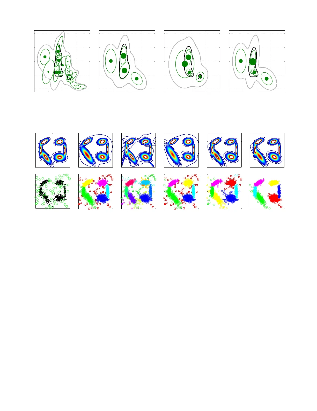
1 Gaussian Mixture Reduction Using Re v erse K ullback-Leibler Di ver gence T ohid Ardeshiri, Umut Orguner , Emre ¨ Ozkan Abstract —W e propose a greedy mixture reduction algorithm which is capable of pruning mixture components as well as merging them based on the Kullback-Leibler divergence (KLD). The algorithm is distinct from the well-known Runnalls’ KLD based method since it is not restricted to merging operations. The capability of pruning (in addition to merging) giv es the algorithm the ability of preserving the peaks of the original mixture during the reduction. Analytical approximations are derived to circumv ent the computational intractability of the KLD which results in a computationally efficient method. The proposed algorithm is compared with Runnalls’ and Williams’ methods in two numerical examples, using both simulated and real world data. The results indicate that the perf ormance and computational complexity of the proposed approach make it an efficient alternative to existing mixture reduction methods. I . I N T RO D U C T I O N Mixture densities appear in v arious problems of the estima- tion theory . The existing solutions for these problems often require efficient strategies to reduce the number of compo- nents in the mixture representation because of computational limits. For example, time series problems can inv olve an ev er increasing number of components in a mixture ov er time. The Gaussian sum filter [1] for nonlinear state estimation; Multi- Hypotheses T racking (MHT) [2] and Gaussian Mixture Prob- ability Hypothesis Density (GM-PHD) filter [3] for multiple target tracking can be listed as examples of the algorithms which require mixture reduction (abbreviated as MR in the sequel) in their implementation. Sev eral methods were proposed in the literature addressing the MR problem. In [4] and [5], the components of the mixture were successi vely mer ged in pairs for minimizing a cost func- tion. A Gaussian MR algorithm using homotopy to av oid local minima was suggested in [6]. Merging statistics for greedy MR for multiple target tracking was discussed in [7]. A Gaussian MR algorithm using clustering techniques w as proposed in [8]. In [9], Crouse et al. presented a surve y of the Gaussian MR algorithms such as W est’ s algorithm [10], constraint optimized weight adaptation [11], Runnalls’ algorithm [12] and Gaussian mixture reduction via clustering [8] and compared them in detail. W illiams and Maybeck [13] proposed using the Integral Square Error (ISE) approach for MR in the multiple hypothesis tracking context. One distinctive feature of the method is the av ailability of exact analytical expressions for e v aluating the cost function between two Gaussian mixtures. Whereas, Runnalls proposed using an upper bound on the Kullback- Leibler diver gence (KLD) as a distance measure between the original mixture density and its reduced form at each step of the reduction in [12]. The motiv ation for the choice of an upper T . Ardeshiri and E. ¨ Ozkan are with the Department of Electrical En- gineering, Link ¨ oping University , 58183 Link ¨ oping, Sweden, e-mail: to- hid,emre@isy .liu.se. U. Orguner is with Department of Electrical and Electronics Engi- neering, Middle East T echnical Univ ersity , 06800 Ankara, T urkey , email: umut@metu.edu.tr . bound in Runnalls’ algorithm is based on the premise that the KLD between two Gaussian mixtures can not be calculated analytically . Runnalls’ approach is dedicated to minimize the KLD from the original mixture to the approximate one, which we refer to here as the F orwar d-KLD (FKLD). This choice of the cost function results in an algorithm, which reduces the number of components only by merging them at each reduction step. In this paper, we propose a KLD based MR algorithm. Our aim is to find an efficient method for minimizing the KLD from the approximate mixture to the original one, which we refer to as the Reverse-KLD (RKLD). The resulting algorithm has the ability to choose between pruning or merging compo- nents at each step of the reduction unlike Runnalls’ algorithm. This enables, for example, the possibility to prune low-weight components while keeping the heavy-weight components un- altered. Furthermore, we present approximations which are required to overcome the analytical intractability of the RKLD between Gaussian mixtures making the implementation fast and efficient. The rest of this paper is organized as follows. In Section II we present the necessary background required for the MR problem we intend to solve in this paper . T wo of the most rel- ev ant works and their strengths and weaknesses are described in Section III. The proposed solution and its strengths are presented in Section IV. Approximations for the fast compu- tation of the proposed div ergence are giv en in Section V. The proposed MR algorithm using the approximations is ev aluated and compared to the alternatives on two numerical examples in Section VI. The paper is concluded in Section VII. I I . B A C K G RO U N D A mixture density is a con ve x combination of (more basic) probability densities, see e.g. [14]. A normalized mixture with N components is defined as p ( x ) = N X I =1 w I q ( x ; η I ) , (1) where the terms w I are positive weights summing up to unity , and η I are the parameters of the component density q ( x ; η I ) . The mixtur e r eduction pr oblem (MRP) is to find an ap- proximation of the original mixture using fewer components. Ideally , the MRP is formulated as a nonlinear optimization problem where a cost function measuring the distance between the original and the approximate mixture is minimized. The optimization problem is solved by numerical solvers when the problem is not analytically tractable. The numerical optimiza- tion based approaches can be computationally quite expensiv e, in particular for high dimensional data, and the y generally suffer from the problem of local optima [6], [9], [13]. Hence, a common alternative solution has been the greedy iterativ e approach. 2 In the gr eedy approach, the number of components in the mixture is reduced one at a time. By applying the same pro- cedure over and ov er again, a desired number of components is reached. T o reduce the number of components by one, a decision has to be made among two types of operations; namely , the pruning and the merging operations. Each of these operations are considered to be a hypothesis in a greedy MRP and is denoted as H I J , I = 0 , . . . , N , J = 1 , . . . , N , I 6 = J . 1) Pruning: Pruning is the simplest operation for reducing the number of components in a mixture density . It is denoted with the hypothesis H 0 J , J = 1 , . . . , N in the sequel. In pruning, one component of the mixture is remov ed and the weights of the remaining components are rescaled such that the mixture integrates to unity . For example, choosing the hypothesis H 0 J , i.e., pruning component J from (1), results in the reduced mixture ˆ p ( x | H 0 J ) , 1 (1 − w J ) N X I =1 I 6 = J w I q ( x ; η I ) . (2) 2) Mer ging: The mer ging operation approximates a pair of components in a mixture density with a single component of the same type. It is denoted with the hypothesis H I J , 1 ≤ I 6 = J ≤ N in the sequel. In general, an optimization problem minimizing a diver gence between the normalized pair of the mixture and the single component is used for this purpose. Choosing the FKLD as the the cost function for mer ging two components, leads to a moment matching operation. More specifically , if the hypothesis H I J is selected, i.e., if the components I and J are chosen to be merged, the parameters of the merged component are found by minimizing the div ergence from the kernel w I q ( x ; η I ) + w J q ( x ; η J ) to a single weighted component ( w I + w J ) q ( x ; η I J ) as follows: η I J = arg min η D K L ( b w I q ( x ; η I ) + b w J q ( x ; η J ) || q ( x ; η )) , where, b w I = w I / ( w I + w J ) , b w J = w J / ( w I + w J ) and D K L ( p || q ) denotes the KLD from p ( · ) to q ( · ) which is defined as D K L ( p || q ) , Z p ( x ) log p ( x ) q ( x ) d x. (3) The minimization of the above cost function usually results in the single component q ( x ; η I J ) whose several moments are matched to those of the two component mixture. The reduced mixture after merging is then giv en as ˆ p ( x |H I J ) , N X K =1 K 6 = I K 6 = J w K q ( x ; η K ) + ( w I + w J ) q ( x ; η I J ) . (4) There are two dif ferent types of greedy approaches in the literature, namely , local and global approaches. The local approaches consider only the merging hypotheses H I J , 1 ≤ I 6 = J ≤ N . In general, the merging hypothesis H I J which provides the smallest diver gence D local ( q ( · ; η I ) || q ( · ; η J )) is selected. This div ergence considers only the components to be merged and neglects the others. Therefore these methods are called local. W ell-known examples of local approaches are giv en in [15], [16]. In the global approaches, both pruning and merging opera- tions are considered. The diver gence between the original and the reduced mixtures, i.e., D global ( p ( · ) || ˆ p ( ·|H I J )) is minimized in the decision. Because the decision criterion for a global approach in volv es all of the components of the original mix- ture, global approaches are in general computationally more costly . On the other hand, since the global properties of the original mixture are taken into account, the y provide better performance. In the follo wing, we propose a global greedy MR method that can be implemented efficiently . I I I . R E L A T E D W O R K In this section, we giv e an ov erview and a discussion for two well-known global MR algorithms related to the current work. A. Runnalls’ Method Runnalls’ method [12] is a global greedy MR algorithm that minimizes the FKLD (i.e., D K L ( p ( · ) || ˆ p ( · ) ). Unfortunately , the KLD between two Gaussian mixtures can not be calculated analytically . Runnalls uses an analytical upper-bound for the KLD which can only be used for comparing merging hypothe- ses. The upper bound B ( I , J ) for D K L ( p ( · ) || ˆ p ( ·|H I J )) , which is given as B ( I , J ) , w I D K L ( q ( x ; η I ) || q ( x ; η I J )) + w J D K L ( q ( x ; η J ) || q ( x ; η I J )) , (5) is used as the cost of merging the components I and J where q ( · , η I J ) is the merged component density . Hence, the original global decision statistics D K L ( p ( · ) || ˆ p ( ·|H I J )) for merging is replaced with its local approximation B ( I , J ) to obtain the decision rule as follows: i ∗ , j ∗ = arg min 1 ≤ I 6 = J ≤ N B ( I , J ) . (6) B. W illiams’ Method W illiams and Maybeck proposed a global greedy MRA in [13] where ISE is used as the cost function. ISE between two probability distributions p ( · ) and q ( · ) is defined by D ISE ( p || q ) , Z | p ( x ) − q ( x ) | 2 d x. (7) ISE has all properties of a metric such as symmetry and triangle inequality and is analytically tractable for Gaussian mixtures. Williams’ method minimizes D ISE ( p ( · ) || ˆ p ( ·|H I J )) ov er all pruning and merging hypotheses, i.e., i ∗ , j ∗ = arg min 0 ≤ I ≤ N 1 ≤ J ≤ N I 6 = J D ISE ( p ( · ) || ˆ p ( ·|H I J )) . (8) C. Discussion In this subsection, first we illustrate the behavior of Run- nalls’ and Willams’ methods on a very simple MR example. Second, we provide a brief discussion on the characteristics observed in the examples along with their implications. Example 1. Consider the Gaussian mixture with two compo- nents given below . p ( x ) = w 1 N ( x ; − µ, 1) + w 2 N ( x ; µ, 1) (9) where µ  2 and w 1 + w 2 = 1 . W e would like to reduce the mixture to a single component and hence we consider the two pruning hypotheses H 01 , H 02 and the merging hypothesis 3 H 12 . The reduced mixtures under these hypotheses are given as ˆ p ( x |H 01 ) = N ( x ; µ, 1) , (10a) ˆ p ( x |H 02 ) = N ( x ; − µ, 1) , (10b) ˆ p ( x |H 12 ) = N ( x ; µ, Σ) , (10c) where µ and Σ are computed via moment matching as µ =( w 2 − w 1 ) µ, (11a) Σ =1 + 4 w 1 w 2 µ 2 . (11b) Noting that the optimization problem µ ∗ , P ∗ = arg min µ,P D K L ( p ( · ) ||N ( · , µ, P )) (12) has the solution µ ∗ = µ and P ∗ = Σ , we see that the density ˆ p ( x |H 12 ) is the best reduced mixture with respect to FKLD. Similarly , Runnalls’ method would select H 12 as the best mixture reduction hypothesis because it considers only the merging hypotheses.  Example 2. W e consider the same MR problem in Example 1 with the Williams’ method. The ISE between the original mixture and the reduced mixture can be written as D ISE ( p ( · ) || ˆ p ( ·|H I J )) + = Z ˆ p ( x |H I J ) 2 d x − 2 Z p ( x ) ˆ p ( x |H I J ) d x (13) where the sign + = means equality up to an additi ve constant independent of H I J . Letting ˆ p ( x |H I J ) = N ( x ; µ I J , Σ I J ) , we can calculate D ISE ( p ( · ) || ˆ p ( ·|H I J )) using (13) as D ISE ( p ( · ) || ˆ p ( ·|H I J )) + = N ( µ I J ; µ I J , 2Σ I J ) − 2 w 1 N ( µ I J ; − µ, 1 + Σ I J ) − 2 w 2 N ( µ I J ; µ, 1 + Σ I J ) . (14) Hence, for the hypotheses listed in (10), we hav e D ISE ( p ( · ) || ˆ p ( ·|H 01 )) + =(1 − 2 w 2 ) N ( µ ; µ, 2) − 2 w 1 N ( µ ; − µ, 2) (15) =(1 − 2 w 2 ) N (0; 0 , 2) − 2 w 1 N ( µ ; − µ, 2) (16) D ISE ( p ( · ) || ˆ p ( ·|H 02 )) + =(1 − 2 w 1 ) N ( − µ ; − µ, 2) − 2 w 2 N ( − µ ; µ, 2) (17) =(1 − 2 w 1 ) N (0; 0 , 2) − 2 w 2 N ( µ ; − µ, 2) (18) D ISE ( p ( · ) || ˆ p ( ·|H 12 )) + = N ( µ ; µ, 2Σ) − 2 w 1 N ( µ ; − µ, 1 + Σ) − 2 w 2 N ( µ ; µ, 1 + Σ) (19) = N (0; 0 , 2Σ) − 2 w 1 N (2 w 2 µ ; 0 , 1 + Σ) − 2 w 2 N (2 w 1 µ ; 0 , 1 + Σ) (20) Restricting ourselves to the case where w 1 = w 2 = 1 / 2 and µ is very large, we can see that D ISE ( p ( · ) || ˆ p ( ·|H 01 )) ≈ − 1 √ 4 π e − µ 2 (21) D ISE ( p ( · ) || ˆ p ( ·|H 02 )) ≈ − 1 √ 4 π e − µ 2 (22) D ISE ( p ( · ) || ˆ p ( ·|H 12 )) ≈ 1 √ 2 π µ  1 √ 2 − 2 √ e  ≈ − 0 . 51 √ 2 π µ . (23) For sufficiently large µ values, it is now easily seen that D ISE ( p ( · ) || ˆ p ( ·|H 12 )) 0 is very small. When µ is sufficiently close to zero, we can express D K L ( ˆ p ( x |H I J ) || p ( x )) using a second- order T aylor series approximation around µ = 0 as follows: D K L ( ˆ p ( x |H I J ) || p ( x )) ≈ 1 2 c I J µ 2 (26) where c I J , ∂ 2 ∂ µ 2 D K L ( ˆ p ( x |H I J ) || p ( x ))     µ =0 . (27) This is because, when µ = 0 , both p ( · ) and ˆ p ( ·|H I J ) are equal to N ( · ; 0 , 1) and therefore D K L ( ˆ p ( x |H I J ) || p ( x )) = 0 . Since D K L ( ˆ p ( x |H I J ) || p ( x )) is minimized at µ = 0 , the first deriv ativ e of D K L ( ˆ p ( x |H I J ) || p ( x )) also v anishes at µ = 0 . The second deriv ative term c I J is given by tedious but straightforward calculations as c I J = Z  ∂ ∂ µ p ( x )    µ =0 − ∂ ∂ µ ˆ p ( x |H I J )    µ =0  2 N ( x ; 0 , 1) d x. (28) Using the identity ∂ ∂ µ N ( x ; µ, 1) = ( x − µ ) N ( x ; µ, 1) (29) we can now calculate c 01 , c 02 and c 12 as c 01 =4 w 2 1 (30a) c 02 =4 w 2 2 , (30b) c 12 =0 . (30c) Hence, when µ is sufficiently small, the RKLD cost function results in the selection of merging operation similar to FKLD and Runnalls’ method.  Example 4. W e consider the same MR problem in Example 1 and 2 when µ is very large. In the following, we calculate the RKLDs for the hypotheses gi ven in (10). • H 01 and H 02 : W e can write the RKLD for H 01 as D K L ( ˆ p ( ·|H 01 ) || p ( · )) = − E H 01 [log p ( x )] − H ( ˆ p ( ·|H 01 )) , (31) where the notation E H I J [ · ] denotes the expectation oper- ation on the argument with respect to the density function ˆ p ( ·|H I J ) and H ( · ) denotes the entropy of the argument density . Under the assumption that µ is very large, we can approximate the expectation E H 01 [log p ( x )] as E H 01 [log p ( x )] , Z N ( x ; µ, 1) × log ( w 1 N ( x ; − µ, 1) + w 2 N ( x ; µ, 1)) d x (32) ≈ Z N ( x ; µ, 1) log ( w 2 N ( x ; µ, 1)) d x (33) = log w 2 − log √ 2 π − 1 2 (34) where we used the fact that ov er the ef fectiv e integration range (around the mean µ ), we have w 2 N ( x ; − µ, 1) ≈ 0 . (35) Substituting this result and the entropy 1 of ˆ p ( ·|H 01 ) into (31) along with, we obtain D K L ( ˆ p ( ·|H 01 ) || p ( · )) ≈ − log w 2 . (36) Using similar arguments, we can easily obtain D K L ( ˆ p ( ·|H 02 ) || p ( · )) ≈ − log w 1 . (37) Noting that the logarithm function is monotonic, we can also see that the approximations giv en on the right hand sides of the above equations are upper bounds for the corresponding RKLDs. • H 12 : W e now calculate a lower bound on D K L ( ˆ p ( x |H 12 ) || p ( x )) and show that this lower bound is greater than both − log w 1 and − log w 2 when µ is sufficiently large. D K L ( ˆ p ( x |H 12 ) || p ( x )) = − E H 12 [log p ( x )] − H ( ˆ p ( ·|H 12 )) (38) W e consider the following facts N ( x ; − µ, 1) ≥ N ( x ; µ, 1) when x ≤ 0 , (39a) N ( x ; µ, 1) ≥ N ( x ; − µ, 1) when x ≥ 0 . (39b) Using the identities in (39) we can obtain a bound on the expectation E H 12 [log p ( x )] as E H 12 [log p ( x )] , E H 12 [log ( w 1 N ( x ; − µ, 1) + w 2 N ( x ; µ, 1))] ≤ Z x ≤ 0 N ( x ; ¯ µ, Σ) log ( N ( x ; − µ, 1)) d x + Z x> 0 N ( x ; ¯ µ, Σ) log ( N ( x ; µ, 1)) d x (40) = − Z x ≤ 0 N ( x ; ¯ µ, Σ)  log √ 2 π + ( x + µ ) 2 2  d x − Z x> 0 N ( x ; ¯ µ, Σ)  log √ 2 π + ( x − µ ) 2 2  d x (41) ≤ − log √ 2 π − Z x ≤ 0 N ( x ; ¯ µ, Σ) x 2 + 2 µx + µ 2 2 d x − Z x> 0 N ( x ; ¯ µ, Σ) x 2 − 2 µx + µ 2 2 d x (42) 1 Entropy of a Gaussian density N ( · , µ, σ 2 ) is equal to log √ 2 π eσ 2 . 5 = − log √ 2 π − ¯ µ 2 + Σ + µ 2 2 − µ Z x ≤ 0 x N ( x ; ¯ µ, Σ) d x + µ Z x> 0 x N ( x ; ¯ µ, Σ) d x (43) = − log √ 2 π − ¯ µ 2 + Σ + µ 2 2 − µ Z x ≤ 0 x N ( x ; ¯ µ, Σ) d x + µ  ¯ µ − Z x ≤ 0 x N ( x ; ¯ µ, Σ)  d x (44) = − log √ 2 π − ¯ µ 2 + Σ + µ 2 2 + µ ¯ µ − 2 µ Z x ≤ 0 x N ( x ; ¯ µ, Σ) d x (45) = − log √ 2 π − ( µ − ¯ µ ) 2 + Σ 2 − 2 µ ¯ µ Φ  − ¯ µ √ Σ  + 2 µ √ Σ φ  − ¯ µ √ Σ  (46) where we have used the result Z ¯ x −∞ x N ( x, µ, Σ) d x = µ Φ  ¯ x − µ √ Σ  − √ Σ φ  ¯ x − µ √ Σ  . (47) Here, the functions φ ( · ) and Φ( · ) denote the probability density function and cumulati ve distribution function of a Gaussian random variable with zero mean and unity variance, respectively . Substituting the upper bound (46) into (38), we obtain D K L ( ˆ p ( x |H 12 ) || p ( x )) ≥ − 1 2 − 1 2 log Σ + ( µ − ¯ µ ) 2 + Σ 2 + 2 µ ¯ µ Φ  − ¯ µ √ Σ  − 2 µ √ Σ φ  − ¯ µ √ Σ  (48) ≈ − 1 2 − 1 2 log  4 w 1 w 2 µ 2  + 2 µ 2  w 1 + ( w 2 − w 1 ) × Φ  w 1 − w 2 √ 4 w 1 w 2  − √ 4 w 1 w 2 φ  w 1 − w 2 √ 4 w 1 w 2   = − 1 2 − 1 2 log  4 w 1 w 2 µ 2  + 2 g ( w 1 , w 2 ) µ 2 (49) for sufficiently large µ values where we used the defini- tions of ¯ µ , Σ and the fact that when µ tends to infinity , we have − ¯ µ √ Σ → w 1 − w 2 √ 4 w 1 w 2 . (50) The coefficient g ( w 1 , w 2 ) in (49) is defined as g ( w 1 , w 2 ) , w 1 + ( w 2 − w 1 )Φ  w 1 − w 2 √ 4 w 1 w 2  − √ 4 w 1 w 2 φ  w 1 − w 2 √ 4 w 1 w 2  . (51) When µ tends to infinity , the dominating term on the right hand side of (49) becomes the last term. By generating a simple plot, we can see that the function g ( w 1 , 1 − w 1 ) is positiv e for 0 < w 1 < 1 , which makes the right hand side of (49) go to infinity as µ tends to infinity . Consequently , the cost of the merging operation exceeds both of the pruning hypotheses for sufficiently large µ v alues. Therefore, the component ha ving the minimum weight is pruned when the components are sufficiently separated.  As illustrated in Example 4, when the components of the mixture are far aw ay from each other , RKLD refrains from merging them. This property of RKLD is known as zer o- for cing in the literature [14, p. 470]. The RKLD between two Gaussian mixtures is analytically intractable except for trivial cases. Therefore, to be able to use RKLD in MR, approximations are necessary just as in the case of FKLD with Runnalls’ method. W e propose such approximations of RKLD for the pruning and merging operations in the following section. V . A P P RO X I M A T I O N S F O R R K L D In sections V -A and V -B, specifically tailored approxima- tions for the cost functions of pruning and merging hypotheses are deri ved respectiv ely . Before proceeding further, we would like to introduce a lemma which is used in the deriv ations. Lemma 1. Let q I ( x ) , q J ( x ) , and q K ( x ) be three pr obability distributions and w I and w J two positive real numbers. The following inequality holds Z q K ( x ) log q K ( x ) w I q I ( x ) + w J q J ( x ) d x ≤ − log ( w I exp( − D K L ( q K || q I )) + w J exp( − D K L ( q K || q J ))) (52) Pr oof. For the proof see Appendix A. A. Appr oximations for pruning hypotheses Consider the mixture density p ( · ) defined as p ( x ) = N X I =1 w I q I ( x ) , (53) where q I ( x ) , q ( x ; η I ) . Suppose we reduce the mixture in (53) by pruning the I th component as follows. ˆ p ( x |H 0 I ) = 1 1 − w I X i ∈{ 1 ··· N }−{ I } w i q i ( x ) . (54) An upper bound can be obtained using the fact that the logarithm function is monotonically increasing as D K L ( ˆ p ( ·|H 0 I ) || p ( · )) = Z ˆ p ( x |H 0 I ) log ˆ p ( x |H 0 I ) p ( x ) d x = Z ˆ p ( x |H 0 I ) log ˆ p ( x |H 0 I ) (1 − w I ) ˆ p ( x |H 0 I ) + w I q I d x ≤ − log (1 − w I ) + Z ˆ p ( x |H 0 I ) log ˆ p ( x |H 0 I ) ˆ p ( x |H 0 I ) d x = − log (1 − w I ) . (55) This upper bound is rather crude when the I th com- ponent density is close to other component densities in the mixture. Therefore we compute a tighter bound on 6 D K L ( ˆ p ( ·|H 0 I ) || p ( · )) using the log-sum inequality [17]. Be- fore we deriv e the upper bound, we first define the following unnormalized density r ( x ) = X i ∈{ 1 ··· N }−{ I ,J } w i q i ( x ) (56) where J 6 = I and R r ( x ) d x = 1 − w I − w J . W e can rewrite the RKLD between ˆ p ( ·|H 0 I ) and p ( · ) as D K L ( ˆ p ( ·|H 0 I ) || p ( · )) = Z 1 1 − w I ( r ( x ) + w J q J ( x )) × log 1 1 − w I ( r ( x ) + w J q J ( x )) r ( x ) + w I q I ( x ) + w J q J ( x ) d x = − log(1 − w I ) + 1 1 − w I Z ( r ( x ) + w J q J ( x )) × log r ( x ) + w J q J ( x ) r ( x ) + w I q I ( x ) + w J q J ( x ) d x. (57) Using the log-sum inequality we can obtain the following expression. D K L ( ˆ p ( ·|H 0 I ) || p ( · )) ≤ − log (1 − w I ) + 1 1 − w I Z r ( x ) log r ( x ) r ( x ) d x + 1 1 − w I Z w J q J ( x ) log w J q J ( x ) w I q I ( x ) + w J q J ( x ) d x = − log (1 − w I ) + w J 1 − w I log( w J ) + w J 1 − w I Z q J ( x ) log q J ( x ) w I q I ( x ) + w J q J ( x ) d x. (58) Applying the result of Lemma 1 on the integral, we can write D K L ( ˆ p ( ·|H 0 I ) || p ( · )) ≤ − log (1 − w I ) − w J 1 − w I log  1 + w I w J exp( − D K L ( q J || q I ))  . (59) Since J is arbitrary , as long as J 6 = I , we obtain the upper bound given below . D K L ( ˆ p ( ·|H 0 I ) || p ( · )) ≤ min J ∈{ 1 ··· N }−{ I }  − log(1 − w I ) − w J 1 − w I log  1 + w I w J exp( − D K L ( q J || q I ))   . (60) The proposed approximate div ergence for pruning component I will be denoted by R (0 , I ) , where 1 ≤ I ≤ N in the rest of this paper . In the following, we illustrate the advantage of the proposed approximation in a numerical example. Example 5. Consider Example 1 with the mixture (9) and the hypothesis (10b). In Figure 1 the exact di ver gence D K L ( p ( ·|H 02 ) || p ( · )) , which is computed numerically , its crude approximation giv en in (55) and the proposed approx- imation R (0 , 2) are sho wn for different values of µ with w 1 = 0 . 8 . Both the exact div ergence and the upper bound R (0 , 2) con verge to − log (1 − w 2 ) when the pruned component has small overlapping probability mass with the other com- ponent. The bound R (0 , 2) brings a significant improvement ov er the crude bound when the amount of overlap between the components increases.  0 0.5 1 1.5 2 2.5 3 3.5 4 0 0.1 0.2 µ Figure 1: The exact di vergence D K L ( p ( ·|H 02 ) || p ( · )) (solid black), the crude upper bound − log (1 − w 2 ) (dotted black) and , the proposed upper bound R (0 , 2) (dashed black) are plotted for different values of µ . B. Appr oximations for mer ging hypotheses Consider the problem of merging the I th and the J th components of the mixture density (53) where the resulting approximate density is giv en as follows. ˆ p ( x |H I J ) = w I J q I J ( x ) + X i ∈{ 1 ··· N }−{ I ,J } w i q i ( x ) . (61) W e are interested in the RKLD between ˆ p ( ·|H I J ) and p ( · ) . T wo approximations of this quantity with dif ferent accuracy and computational cost are giv en in sections V -B1 and V -B2. 1) A simple upper bound: W e can compute a bound on D K L ( ˆ p ( ·|H I J ) || p ( · )) as follows: D K L ( ˆ p ( ·|H I J ) || p ( · )) = Z ( r ( x ) + w I J q I J ( x )) log r ( x ) + w I J q I J ( x ) r ( x ) + w I q I ( x ) + w J q J ( x ) d x ≤ Z r ( x ) log r ( x ) r ( x ) d x + Z w I J q I J ( x ) log w I J q I J ( x ) w I q I ( x ) + w J q J ( x ) d x = w I J log w I J + w I J Z q I J ( x ) log q I J ( x ) w I q I ( x ) + w J q J ( x ) d x (62) where the log-sum inequality is used and r ( x ) is defined in (56). Using Lemma 1 for the second term on the right hand side of (62), we obtain D K L ( ˆ p ( ·|H I J ) || p ( · )) ≤ w I J log w I J − w I J × log ( w I exp( − D K L ( q I J || q I )) + w J exp( − D K L ( q I J || q J ))) . (63) 2) A variational appr oximation: The upper bound deri ved in the previous subsection is rather loose particularly when the components q I and q J are far from each other . This is because of the replacement of the second term in (62) with its approximation in (63) which is a function of D K L ( q I J || q I ) and D K L ( q I J || q J ) . For a brief description of the problem consider D ( q I J || w I q I + w J q J ) , Z q I J ( x ) log q I J ( x ) w I q I ( x ) + w J q J ( x ) d x (64) and its approximation using Lemma 1 given as − log ( w I exp( − D K L ( q I J || q I )) + w J exp( − D K L ( q I J || q J ))) . 7 The integral in volv ed in the calculation of D K L ( q I J || q I ) grows too much (compared to the original div ergence D ( q I J || w I q I + w J q J ) ) ov er the support of q J because q I J shares significant support with q J . Similarly , the integral in D K L ( q I J || q J ) grows too much (compared to the original di- ver gence D ( q I J || w I q I + w J q J ) ) o ver the support of q I because q I J shares significant support with q I . T o fix these prob- lems, we propose the following procedure for approximating D ( q I J || w I q I + w J q J ) using the boundedness of the component densities. In the proposed variational approximation, first, an upper bound on D ( q I J || w I q I + w J q J ) is obtained using the log-sum inequality as D ( q I J || w I q I + w J q J ) ≤ Z αq I J log αq I J w I q I d x + Z (1 − α ) q I J log (1 − α ) q I J w J q J d x (65) = α Z q I J log q I J q I d x + α log α w I + (1 − α ) Z q I J log q I J q J d x + (1 − α ) log 1 − α w J (66) where 0 < α < 1 . Second, a switching function is applied to the integrals in (66) as follows. D ( q I J || w I q I + w J q J ) ≈ Z αq I J ( x )  1 − q J ( x ) q max J  log q I J ( x ) q I ( x ) d x + α log α w I + Z (1 − α ) q I J ( x )  1 − q I ( x ) q max I  log q I J ( x ) q J ( x ) d x + (1 − α ) log 1 − α w J (67) where q max I , max x q I ( x ) . Here, the multipliers  1 − q J ( x ) q max J  , and  1 − q I ( x ) q max I  in the integrands are equal to almost unity ev erywhere except for the support of q J and q I respectiv ely , where they shrink to zero. In this way , the excessi ve growth of the div ergences in the upper bound are reduced. Note also that the terms q max J and q max I are readily a vailable as the maximum v alues of the Gaussian component densities. Finally , the minimum of the right hand side of (67) is obtained with respect to α . The optimization problem can be solved by taking the deriv ati ve with respect to α and equating the result to zero which gives the following optimal value α ∗ = w I exp( − V ( q I J , q J , q I )) w I exp( − V ( q I J , q J , q I )) + w J exp( − V ( q I J , q I , q J ))) , where V ( q K , q I , q J ) , Z q K ( x )  1 − q I ( x ) q max I  log q K ( x ) q J ( x ) d x. (68) A closed form expression for the quantity V ( q K , q I , q J ) is giv en in Appendix B. Substituting α ∗ into (67) results in the following approximation for D ( q I J || w I q I + w J q J ) . D ( q I J || w I q I + w J q J ) ≈ − log ( w I exp( − V ( q I J , q J , q I )) + w J exp( − V ( q I J , q I , q J ))) (69) 0 0.5 1 1.5 2 2.5 3 3.5 4 0 0.1 0.2 µ Figure 2: The exact di vergence D K L ( ˆ p ( ·|H 12 ) || p ( · )) (solid blue), the simple approximation given in (63) (dotted blue), and the proposed approximation R (1 , 2) (dashed blue) are plotted for different values of µ . In addition, the exact pruning div ergence D K L ( ˆ p ( ·|H 02 ) || p ( · )) (solid black), the crude prun- ing upper bound − log(1 − w 2 ) (dotted black) and the proposed pruning upper bound R (0 , 2) (dashed black) are plotted. When we substitute this approximation into (62), the proposed approximate diver gence for merging becomes D K L ( ˆ p ( ·|H I J ) || p ( · )) ≈ w I J log w I J − w I J × log ( w I exp( − V ( q I J , q J , q I )) + w J exp( − V ( q I J , q I , q J ))) . (70) The proposed approximate div ergence for merging compo- nents I and J in (70) will be denoted by R ( I , J ) in the rest of this paper . Example 6. Consider Example 1 with the mixture (9) and the hypothesis (10c). In Figure 2, the exact di vergence D K L ( ˆ p ( ·|H 12 ) || p ( · )) , which is computed numerically , the simple approximation giv en in (63) and the proposed ap- proximation R (1 , 2) are shown for different values of µ with w 1 = 0 . 8 . Note that the range at which approximations are interesting to study is where D K L ( ˆ p ( ·|H 12 ) || p ( · )) < − log (1 − w 2 ) . This is because of the fact that when D K L ( ˆ p ( ·|H 12 ) || p ( · )) > − log (1 − w 2 ) , pruning hypothesis H 02 will be selected. The range of axes in Figure 2 is chosen according to the aforementioned range of interest. The proposed variational approximation R (1 , 2) performs very well compared to the simple upper bound which grows too fast with increasing µ v alues. Furthermore, the points where the curves of exact pruning and merging div ergences cross (the crossing point of the solid lines in Figure 2) is close to the crossing point of the curves of best approximation of these two quantities (the crossing point of the dashed lines in Figure 2).  The approximate MRA proposed in this work uses the two approximations for pruning and merging div ergences, R ( I , J ) where 0 ≤ I ≤ N , 1 ≤ J ≤ N , and I 6 = J . W e will refer to this algorithm as Approximate Re verse Kullback-Leibler (ARKL) MRA. The precision of ARKL can be traded for less computation time by replacing the approximations for pruning and merging hypotheses by their less precise counterparts giv en in sections V -A and V -B. V I . S I M U L A T I O N R E S U LT S In this section, the performance of the proposed MRA, ARKL, is compared with Runnalls’ and Williams’ algorithms in two examples. In the first e xample, we use the real world data from terrain-referenced na vigation. In the second 8 469 470 471 472 473 160 161 162 163 164 (a) Original density 469 470 471 472 473 160 161 162 163 164 (b) Reduced by Runnalls’ 469 470 471 472 473 160 161 162 163 164 (c) Reduced by Williams’ 469 470 471 472 473 160 161 162 163 164 (d) Reduced by ARKL Figure 3: The data for the original mixture density is courtesy of Andrew R. Runnalls and shows the horizontal position errors in the terrain-referenced navigation. The unit of axes is in kilometers and are represented in UK National Grid coordinates. The original mixture in 3a is reduced in 3b, 3c and 3d using different MRAs. −10 0 10 −10 −5 0 5 10 −10 0 10 −10 −5 0 5 10 (a) Original density −10 0 10 −10 −5 0 5 10 −10 0 10 −10 −5 0 5 10 (b) 6 clusters by EM −10 0 10 −10 −5 0 5 10 −10 0 10 −10 −5 0 5 10 (c) 15 clusters by EM −10 0 10 −10 −5 0 5 10 −10 0 10 −10 −5 0 5 10 (d) Runnalls’ −10 0 10 −10 −5 0 5 10 −10 0 10 −10 −5 0 5 10 (e) Williams’ −10 0 10 −10 −5 0 5 10 −10 0 10 −10 −5 0 5 10 (f) ARKL Figure 4: Results of the clustering example. In the top row , the contour plots of the GMs are giv en. The bottom row presents the corresponding data points associated to the clusters in different colors. example, we ev aluate the MRAs on a clustering problem with simulated data. A. Example with real world data An example that Runnalls used in [12, Sec.VIII] is re- peated here for the comparison of ARKL with Runnalls’ and W illiams’ algorithms. In this example a Gaussian Mixture (GM) consisting of 16 components which represents a terrain- referenced navigation system’ s state estimate is reduced to a GM with 4 components. The random variable whose distribu- tion is represented by a GM is 15 dimensional but only two elements of it (horizontal components of position error) are visualized in [12, Sec.VIII]. W e use the marginal distribution of the visualized random variables to illustrate the differences of MRAs. Figure 3a sho ws the original mixture density . Each Gaussian component is represented by its mean, its weight, which is proportional to the area of the marker representing the mean, and its 50 percentile contour (an elliptical contour enclosing the 50% probability mass of the Gaussian density). The thick gray curves in Figure 3 are the 95 percentile contour and the thick black curves show the 50 percentile contour of the mixture density . In Figures 3b and 3c, the reduced GMs using Runnalls’ and W illiams’ methods are illustrated by their components and their 50 and 95 percentile contours 2 . Figure 3d illustrates the result of the ARKL algorithm. W illiams’ algorithm is the only algorithm that preserves the second mode in the 50 percentile contour , but has distorted the 95 percentile contour the most. The 50 percentile contour of ARKL is the most similar to the original density . Also, the shape of the 95 percentile contour is well preserved by ARKL as well as Runnalls’. An interesting observ ation is that the 95 percentile contour for ARKL has sharper corners than that obtained by Runnalls’ algorithm which is a manifestation of the pruning decisions (zero-forcing) in ARKL as opposed to the merging (zero-av oiding) decisions in Runnalls’ algorithm for small-weight components. The MRAs are compared quantitativ ely in terms of di- ver gences, FKLD, RKLD and ISE in T able I. The FKLD and RKLD are calculated using MC integration while ISE is calculated using its analytical expression. Naturally , MRAs obtain the least div ergence with their respectiv e criteria. That is, Runnalls’ algorithm obtains the lo west FKLD, W illiams’ algorithm obtains the lowest ISE, and ARKL obtains the lowest RKLD. In terms of ISE, Runnalls’ algorithm and 2 The difference between Figures 3b and 3c and [12, Fig.2] is because of the exclusion of the pruning hypotheses in implementation of Williams’ algorithm in [12, Fig.2] and the fact that we are only using the marginal distribution of the two position error elements in the random variable. 9 T able I: Comparison of MRAs in terms of the diver gence between the reduced mixture density and the original density . Mixture Reduction Algorithms Divergence Measures W illiams’ Runnalls’ ARKL ISE 0.0175 0.0255 0.0271 FKLD 0.1177 0.0665 0.3024 RKLD 0.1325 0.1234 0.0340 ARKL seems to be very close to each other which implies that for large weight components (large probability mass), these algorithms work similarly . In terms of FKLD, the W illiams’ algorithm obtains much closer a value to that of Runnalls’ algorithm than ARKL which means that the mer ging (zero-av oiding) properties of W illiams’ algorithm is closer to Runnalls’ algorithm. Finally , in terms of RKLD, Williams’ algorithm and Runnalls’ algorithm have similar and larger values than ARKL. This makes us conclude that pruning (zero- forcing) ability of W illiams’ algorithm is as bad as Runnalls’ algorithm for this example. B. Robust clustering In the following, we illustrate the necessity of the pruning capability of an MRA (as well as merging) using a clustering example in an environment with spurious measurements. Consider a clustering problem where the number of clusters N c is known a priori. Also, assume that the data is corrupted by a small number of spurious measurements, which are the data points not belonging to any of the true clusters and can be considered to be outliers. The clustering task is to retriev e N c clusters from the corrupted data. A straightforward approach to this problem is to neglect the existence of the spurious measurements and cluster the corrupted data directly into N c clusters. Since this solution does not take the spurious measurements into account, the re- sulting clusters might not represent the true data satisfactorily . Another solution to the problem is to first cluster the data points into N > N c clusters and then reduce the number of clusters to N c . When GMs are used for clustering, an appropriate MRA can be used to reduce the number of clusters (component densities) from N to N c . An MRA which can prune components with small weights which are distant from the rest of the probability mass is a good candidate. On the other hand, an MRA which reduces the mixture using only merging operations is not preferable because the spurious measurements would corrupt the true clusters. Furthermore, when a component is being pruned/discarded the data points associated to the pruned component density can also be discarded as potential spurious data points. Consequently , it is expected that ARKL and W illiams’ algorithm might perform better than Runnalls’ algorithm in this example because of their pruning capability . In this simulation n = 1000 data points are generated from a Gaussian mixture with N c = 6 components, { x i } n i =1 ∼ p ( x ) = P N c j =1 w j N ( x ; µ j , Σ j ) where the parameters of p ( x ) are gi ven in T able II. The data points are augmented with m = 100 spurious data points sampled uniformly from a multiv ariate uniform distribution over the square region A , i.e., { y i } m i =1 ∼ U ( A ) , where the center of the square is at the origin and each side is 20 units long. The clustering results of the following methods are presented. • The direct clustering of the corrupted data, i.e., z = {{ x i } n i =1 , { y i } m i =1 } into 6 clusters using Expectation T able II: The parameters of the original mixture density used in the example of section VI-B and presented in Figure 4a. 1 ≤ j ≤ 3 4 ≤ j ≤ 6 j w j µ j Σ j j w j µ j Σ j 1 0 . 2  − 5 5   1 0 . 5 0 . 5 0 . 5  4 0 . 2  − 4 − 4   2 − 2 − 2 3  2 0 . 2  4 5   1 0 . 2 0 . 2 0 . 5  5 0 . 1  − 7 0   0 . 1 0 0 3  3 0 . 2  4 − 4   2 0 0 1  6 0 . 1  7 0   0 . 1 0 0 3  Maximization (EM) algorithm [14, Chapter 9]. • The clustering of the corrupted data into 15 clusters using EM algorithm. • The clustering of the corrupted data into 15 clusters using EM algorithm and then reduction to 6 clusters using – Runnalls’ algorithm – Williams’ algorithm – ARKL In Figure 4 the contour plots of the densities along with the corresponding data points are illustrated. In Figure 4a (top) the contour plots of the true clusters are plotted. The true (black) and spurious (green) data points are sho wn in Figure 4a (bottom). In Figure 4b, the contour plot (top) of the GM obtained by EM algorithm clustering the corrupted data directly into 6 clusters is shown with the corresponding cluster data points (bottom). The direct clustering of the corrupted data into 6 components results in a clustering which does not capture all of the true clusters since a spurious cluster with a large cov ariance is formed out of spurious data points (red data points). As a remedy , the data is first clustered into 15 clusters (see Figure 4c) using EM algorithm and the resulting 15- component GM is then reduced to 6 components using Run- nalls’ algorithm (Figure 4d), W illiams’ algorithm (Figure 4e) and ARKL (Figure 4f). W ith these algorithms, when a com- ponent is pruned (which might be the case for W illiams’ algorithm and ARKL), the data points associated with that component are discarded as well. On the other hand, when a component is merged with another component, data points associated with the merged component are reassigned to the updated set of clusters according to their proximity measured by Mahalanobis distance. The final clustering obtained by Runnalls’ algorithm is almost the same as the result obtained by the EM algorithm with 6 clusters. This observation is in line with the Maximum Likelihood interpretation/justification of the Runnalls’ algo- rithm given in [12]. W illiams’ algorithm and ARKL capture the shape of the original GM and the 6 clusters much better than Runnalls’ algorithm because these two algorithms can prune (as well as merge) while Runnalls’ algorithm can only merge. While some of the spurious clusters/measurements are merged with the true clusters by W illiams’ algorithm, almost all spurious clusters/measurements are pruned by ARKL. Lastly , as aforementioned, the computation complexity of W illiams’ method is O ( N 4 ) while reducing a mixture with N components to a mixture with N − 1 components. Howe ver , Runnalls’ and the ARKL methods hav e O ( N 2 ) complexity , which makes them preferable when a fast reduction algorithm is needed for reducing a mixture with many components. 10 V I I . C O N C L U S I O N W e in vestigated using the rev erse Kullback-Leibler diver - gence as the cost function for greedy mixture reduction. Pro- posed analytical approximations for the cost function results in an ef ficient algorithm which is capable of both merging and pruning components in a mixture. This property can help preserving the peaks of the original mixture after the reduction and it is missing in FKLD based methods. W e compared the method with two well-known mixture reduction algorithms and illustrated its advantages both in simulated and real data scenarios. R E F E R E N C E S [1] D. L. Alspach and H. W . Sorenson, “Nonlinear Bayesian estimation using Gaussian sum approximations, ” IEEE T rans. Autom. Control , vol. 17, no. 4, pp. 439–448, Aug. 1972. [2] S. Blackman and R. Popoli, Design and Analysis of Modern T racking Systems . Artech House, 1999. [3] B.-N. V o and W .-K. Ma, “The Gaussian mixture probability hypothesis density filter, ” IEEE T rans. Signal Process. , vol. 54, no. 11, pp. 4091– 4104, Nov . 2006. [4] D. Salmond, “Mixture reduction algorithms for target tracking, ” in Pr oceedings of IEE Colloquium on State Estimation in Aer ospace and T racking Applications , London, UK, Dec. 1989, pp. 7/1–7/4. [5] D. J. Salmond, “Mixture reduction algorithms for point and extended object tracking in clutter , ” IEEE Tr ans. Aerosp. Electr on. Syst. , vol. 45, no. 2, pp. 667–686, Apr . 2009. [6] M. F . Huber and U. D. Hanebeck, “Progressive Gaussian mixture reduction, ” in Proceedings of the 11th International Conference on Information Fusion , Cologne, Germany , Jul. 2008. [7] T . Ardeshiri, U. Orguner, C. Lundquist, and T . B. Sch ¨ on, “On mixture reduction for multiple target tracking, ” in Proceedings of the 15th International Conference on Information Fusion , Jul. 2012, pp. 692– 699. [8] D. Schieferdecker and M. F . Huber, “Gaussian mixture reduction via clustering, ” in Proceedings of the 12th International Conference on Information Fusion , Seattle, W A, Jul. 2009, pp. 1536–1543. [9] D. F . Crouse, P . Willett, K. Pattipati, and L. Svensson, “ A look at Gaussian mixture reduction algorithms, ” in Proceedings of the 14th International Confer ence on Information Fusion , Jul. 2011. [10] M. W est, “ Approximating posterior distributions by mixtures, ” Journal of the Royal Statistical Society (Ser . B) , vol. 54, pp. 553–568, 1993. [11] H. D. Chen, K. C. Chang, and C. Smith, “Constraint optimized weight adaptation for Gaussian mixture reduction, ” vol. 7697, Apr . 2010, pp. 76 970N–1–76 970N–10. [12] A. R. Runnalls, “Kullback-Leibler approach to Gaussian mixture reduc- tion, ” IEEE T rans. Aer osp. Electr on. Syst. , vol. 43, no. 3, pp. 989–999, Jul. 2007. [13] J. L. W illiams and P . S. Maybeck, “Cost-function-based hypothesis control techniques for multiple hypothesis tracking, ” Mathematical and Computer Modelling , vol. 43, no. 9-10, pp. 976–989, May 2006. [14] C. M. Bishop, P attern Recognition and Machine Learning . NJ: Springer-V erlag, 2006. [15] D. J. Salmond, “Mixture reduction algorithms for target tracking in clutter , ” in Pr oceedings of SPIE: Signal and Data Pr ocessing of Small T argets , vol. 1305, 1990, pp. 434–445. [16] K. Granstr ¨ om and U. Orguner , “On the reduction of Gaussian in verse Wishart mixtures, ” in Pr oceedings of the 15th International Confer ence on Information Fusion , Jul. 2012, pp. 2162–2169. [17] T . S. Han and K. Kobayashi, Mathematics of Information and Coding , ser . Translations of Mathematical Monographs. American Mathematical Society , 2007. [18] J. R. Hershey and P . A. Olsen, “ Approximating the Kullback Leibler div ergence between Gaussian mixture models, ” in Proceedings of IEEE International Conference on Acoustics, Speech and Signal Processing , vol. 4, Apr . 2007, pp. IV –317–IV –320. A P P E N D I X A. Pr oof of Lemma 1 In the proof of Lemma 1 we use the same approach as the one used in [18, Sec. 8]. Let 0 < α < 1 . Using the log-sum inequality we can obtain an upper bound on the left hand side of (52) as Z q K log q K w I q I + w J q J d x = Z ( αq K + (1 − α ) q K ) log αq K + (1 − α ) q K w I q I + w J q J d x ≤ Z αq K log αq K w I q I d x + Z (1 − α ) q K log (1 − α ) q K w J q J d x = α Z q K log q K q I d x + α log α w I + (1 − α ) Z q K log q K q J d x + (1 − α ) log 1 − α w J = αD K L ( q K || q I ) + α log α w I + (1 − α ) D K L ( q K || q J ) + (1 − α ) log 1 − α w J . (71) The upper bound can be minimized with respect to α to obtain the best upper bound. The minimum is obtained by taking the deriv ativ e of (71) with respect to α ; equating the result to zero and solving for α , which giv es α ∗ = w I exp( − D K L ( q K || q I )) w I exp( − D K L ( q K || q I )) + w J exp( − D K L ( q K || q J )) . Substituting α ∗ into (71) gives the upper bound in (52). B. Derivation of V ( q K , q I , q J ) Let q K ( x ) = N ( x ; µ K , Σ K ) , q I ( x ) = N ( x ; µ I , Σ I ) and q J ( x ) = N ( x ; µ J , Σ J ) and x ∈ R k . The integral V ( q K , q I , q J ) can be written as V ( q K , q I , q J ) , Z q K  1 − q I q max I  log q K q J d x = D K L ( q K || q J ) − 1 q max I Z q K q I log q K q J d x = D K L ( q K || q J ) − (2 π ) k/ 2 | Σ I | 1 / 2 N ( µ I ; µ K , Σ K + Σ I ) ×  Z N ( x ; µ ∗ , Σ ∗ ) log q K d x − Z N ( x ; µ ∗ , Σ ∗ ) log q J d x  =0 . 5 log | Σ K | | Σ J | − 0 . 5 T r [Σ − 1 J (Σ J − Σ K − ( µ J − µ K )( µ J − µ K ) T )] − (2 π ) k/ 2 | Σ I | 1 / 2 N ( µ I ; µ K , Σ K + Σ I )  − 0 . 5 log | 2 π Σ K | − 0 . 5 T r [Σ − 1 K (Σ ∗ + ( µ K − µ ∗ )( µ K − µ ∗ ) T )] + 0 . 5 log | 2 π Σ J | + 0 . 5 T r [Σ − 1 J (Σ ∗ + ( µ J − µ ∗ )( µ J − µ ∗ ) T )]  . where we use the following well-kno wn results for Gaussian distributions. • Diver gence D K L ( N ( x ; µ K , Σ K ) ||N ( x ; µ J , Σ J )) = 0 . 5 log | Σ K | | Σ J | − 0 . 5 T r [Σ − 1 J (Σ J − Σ K − ( µ J − µ K )( µ J − µ K ) T )] . (72) • Multiplication N ( x ; µ I , Σ I ) N ( x ; µ K , Σ K ) = N ( µ K ; µ I , Σ I + Σ K ) × N ( x ; µ ∗ , Σ ∗ ) (73) 11 where µ ∗ = µ I + Σ I (Σ I + Σ K ) − 1 ( µ K − µ I ) , (74) Σ ∗ = Σ I − Σ I (Σ I + Σ K ) − 1 Σ I . (75) • Expected Logarithm Z N ( x ; µ I , Σ I ) log N ( x ; µ J , Σ J ) d x = − 0 . 5 log | 2 π Σ J | − 0 . 5 T r [Σ − 1 J (Σ I + ( µ J − µ I )( µ J − µ I ) T )] . (76) • Maximum V alue q max I = (2 π ) − k/ 2 | Σ I | − 1 / 2 . (77)