Probabilistic Power Flow Computation via Low-Rank and Sparse Tensor Recovery

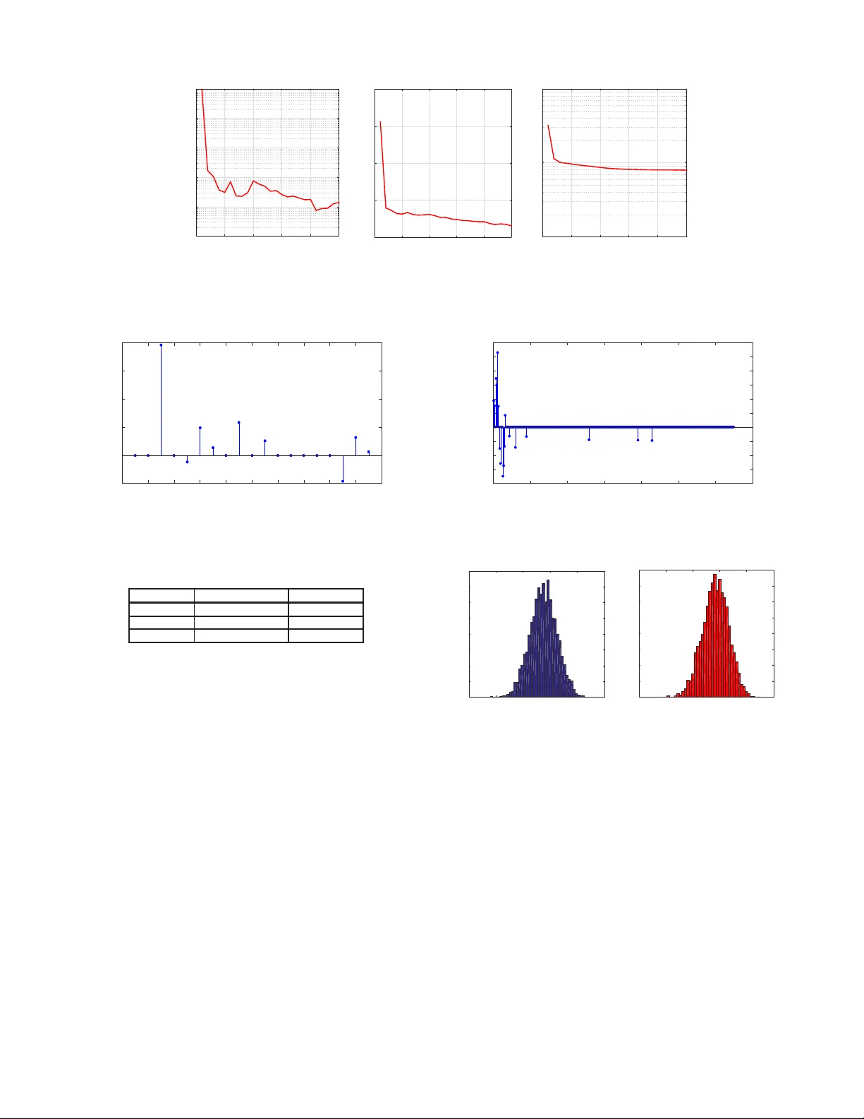
IEEE TRANSACTIONS ON PO WER SYSTEMS, VOL. , NO. , XX 20XX 1 Probabilistic Po wer Flo w Computation via Lo w-Rank and Sparse T ensor Reco v ery Zheng Zhang, Hung Dinh Nguy en, K onstantin T uritsyn and Luca Daniel Abstract —This paper presents a tensor -reco very method to solve probabilistic p ower flow problems. Ou r app roach generates a high-dimensional and sparse generalized polynomial-chaos expansion that provides useful statistical informatio n . The result can also speed up other essential routines in powe r systems (e.g., stochastic planning, operations and controls). Instead of simulating a powe r flo w equation at all quadrature points, our approach only simulates an extreme ly small subset of samples. W e suggest a model to exploit th e underlying low- rank and sparse structure of hi gh-dimensional simulation data arrays, making our techn ique applicable to p ower systems with many random parameters. W e also present a numerical method to solve the resulting nonlinear optimization problem. Our algorithm is i mplemented in MA TLAB and is v erified by sev eral benchmarks in MA TPO WER 5 . 1 . Accurate results are obtained f or p ower systems wi th u p to 50 ind ependent random parameters, with a speedup factor u p to 9 × 10 20 . Index T erms —Power flow , power system, stochastic collocation, tensors, polynomial chaos, uncertainty , optimization. I . I N T R O D U C T I O N R EALISTIC po wer systems are affected by various unce r- tainties, such as the rand omness of generation s and load s, insufficient knowledge a bout n etwork para meters, and n oisy measuremen t [1]– [14]. Uncer tainties may increase in future power systems, since many renew ables highly depen d on the uncertain weathe r conditio ns [6], [9]. These uncertain ties must be considered in sim ulation, such that subseq uent tasks can be completed in an efficient and robust way . This work investigates th e p robabilistic p ower flow prob- lem [2], wh ich quan tifies the uncertainties of bus voltages and line flows u nder uncertain loads, generations or network parameters. Cur rently , this problem is routinely solved in a numb er of decision -making pro cedures. Exa mples in clude transmission expansion and plannin g under long-term u n- certainties in renewables p enetration and regulatio n p olicies [15], [16]. In o perations, the oper ators assess the secur ity of the system an d calculate A vailable T ran sfer Capability using random scenario sampling [17] where the ability to a verage the steady state solution over a large number of ran dom scenarios is essential for secure power oper ations. Probabilistic power flow problem s hav e be en solved by Monte Carlo and many analytical method s (inclu ding multi- linearization [10], the comulant m ethod [11], fuz zy load flow analysis [1 2], and so for th). Recently , poin t estimation has Z. Zhang w as with Massachusetts Instit ute of T echnolog y (MIT), Cam- bridge, MA 02139, USA. He is now with Argonne Natio nal Laboratory , Lemont, IL 60439. E-mail: z zhang@mit .edu. H. D. Nguye n, K. T uritsyn and L. Daniel are with MIT , Cambridge, MA 02139, USA. E-mail s: { hunghtd, turitsyn , luca } @mit.edu. become a pop ular technique for proba bilistic power flo w analysis [4]– [8]. This meth od assumes th e solutio n b eing a summation o f so me u niv ariate fun ctions, th en it compu tes the moments using a set of one-dimension al quad rature points. Stochastic spectral meth ods [ 18] ha ve emerged as a promis- ing techn ique fo r the uncertainty analysis of many engine ering problem s including power systems [13], [14], [19], [2 0]. They appr oximate the stochastic solution by a gener alized polyno mial-chaos expansion [21]. Th is r epresentation can provide various statistical info rmation (e. g., mo ments an d probab ility density function) ; it can also ac celerate many stochastic pro blems in power systems (e.g., stoch astic unit commitmen t [9] an d p arameter inf erence [22]), whereas p revi- ous appro aches generally cannot. Howe ver, stochastic spectral methods may req uire lots o f basis functio ns and simulatio n samples for problems with ma ny uncertainties. In the uncer- tainty quantificatio n commu nity , some techn iques b ased on compressed sensing [23], [24], proper gener alized d ecompo si- tion [25], [26] and tensor -tr ain deco mposition [20], [ 27], [28] have b een developed fo r high -dimension al p roblems. This paper develops an alternativ e stochastic spectral method to solve pr obabilistic power flow pr oblems with possi- bly high-d imensional ran dom parameters. Our main contribu- tions are summ arized as the follo wing : i) W e use tenso rs [2 9] (i.e., hig h-dimen sional data arrays) to represent the hu ge set o f data samples r equired in stochastic simulation. With a tensor format, we pro pose a low-rank and spar se tensor recovery scheme to g enerate a high -dimension al and sparse appro xi- mation while using an extremely small su bset of quadr ature samples. ii) W e present the detailed n umerical implemen ta- tion of th e tensor recovery meth od. Our algo rithm relies on alternating minim ization and the alternating direction metho d of multipliers ( ADMM) [30]. Although only locally optimal solutions are guaran teed, the developed solver p erforms well for many practical cases. W e demonstra te the perf ormance of the prop osed techniqu e with nu merical simulation s on 3 benchm arks in MA TPO WER 5 . 1 [31]. I I . P RO B L E M F O R M U L A T I O N A. Pr o babilistic P ower Flow Pr oblem A steady-state power system with un certainties can be described with parameterized power flo w equations: P i ( ξ ) = n P k =1 V i ( ξ ) V k ( ξ ) ( G ik cos θ ik ( ξ ) + B ik sin θ ik ( ξ )) Q i ( ξ ) = n P k =1 V i ( ξ ) V k ( ξ ) ( G ik sin θ ik ( ξ ) − B ik cos θ ik ( ξ )) (1) where P i , Q i , V i , θ i are the acti ve and reactiv e power , v oltage magnitud e and ang le at load b us i , respectiv ely; G ik and B ik are conduc tances and susceptances; θ ik = θ i − θ k is the v oltage angle difference between buses i and k . W e employ rand om parameter s ξ =[ ξ 1 , · · · , ξ d ] ∈ R d to describe the un certainties of load power con sumptions th at further influence bus voltages an d ang les. After co mputing V i ’ s and θ i ’ s, an ou t of interest y (e.g., the line flo ws) ca n be easily extracted. Obviously y also depen ds on ξ a nd thus can be written as y = g ( ξ ) . W e assume that a determ inistic solver is av ailable to solve (1) giv en a samp le of ξ . F or simplicity , we assume th at all elements of ξ are mutually in depend ent, then their joint pro bability density fu nction is ρ ( ξ ) = d Q k =1 ρ k ( ξ k ) , where ρ k ( ξ k ) is th e ma rginal probability density fun ction of ξ k . Moreover , the slack bus is assigned to com pensate fo r the variations of loads a nd losses. B. Stochastic Collocation Method If the power flow problem is s olvable, and y = g ( ξ ) smo othly depend s o n ξ , th en we can app roximate y by a trun cated generalized p olynomia l-chaos expan sion [21] y = g ( ξ ) ≈ X | α |≤ p c α Ψ α ( ξ ) , with Ψ α ( ξ ) = d Y k =1 φ k,α k ( ξ k ) . (2) The multiv ariate polyn omial b asis Ψ α ( ξ ) is indexed b y α =[ α 1 , · · · , α d ] ∈ N d , with the total polyno mial d egree | α | = d P k =1 | α k | ≤ p . The total number of basis functions is K = ( p + d )! p ! d ! . (3) As shown in Appen dix A , the degree- α k univ ariate polyn o- mials { φ k,α k ( ξ k ) } p α k =0 are orthon ormal to each other . There- fore, th e multiv ariate b asis fun ctions are also orthono rmal, and c α can b e comp uted with pro jection c α = Z R d Ψ α ( ξ ) g ( ξ ) ρ ( ξ ) d ξ . (4) This integral ca n be e valuated by a p roper quad rature ru le which req uires computin g g ( ξ ) at a set o f samples. C. Integr ation Rules an d Curse of Dimensionality Among d ifferent quadratu re r ules [32]–[34], this work considers comp uting c α by a ten sor-rule Ga uss quadra ture method. First, u se G auss quadrature [3 5] ( in Appendix B) to decide m quadratu re samp les and weig hts  ξ i k k , w i k k  m i k =1 for ξ k . Next, we compute c α by a tensor rule c α ≈ m X i 1 =1 · · · m X i d =1 g ( ξ i 1 1 , · · · , ξ i d d ) d Y k =1 φ k,α k ( ξ i k k ) w i k k . (5) This metho d requires simu lating the power flo w eq ua- tion m d times, and obviously it o nly works well f or low- dimensiona l pro blems (e.g ., when d is below 5 or 6 ). Sp arse grid has been applied to simulate po wer sy stems [ 13], wh ich can compute (4) with abou t 2 p K samples for high- dimensiona l cases [19]. In this pap er , we aim to use only < K samp les from a tensor rule to compute (4). Fig. 1. Demonstration of vect ors (l eft), matrices (middle) and tensors (right). I I I . A T E N S O R - R E C OV E RY A P P RO A C H This section presents o ur ten sor-recovery m ethod to solve high-d imensional probabilistic power flow p roblems. A. T ensor Rep r esentation s of (5) As a generalization of vector s an d matrices, a tensor A ∈ R m 1 ×···× m d represents a high-dim ensional data array [ 29]. The number of dimension s, d , is called the mo de o f a tensor; m k is th e size of the k -th dimen sion. Given index i = ( i 1 , · · · , i d ) (with integer i k ∈ [1 , m k ] ), we can specify one element A ( i ) . Fig. 1 shows a 1 -mode tensor (i.e., vector), a 2 - mode tensor (i.e., matrix) and a 3 -mode tensor . First, we define a d -m ode tensor G ∈ R m ×···× m G ( i ) = g ( ξ i 1 1 , · · · , ξ i d d ) . (6) Next, for every ξ k and its degree- α k polyno mial φ k,α k ( ξ k ) , we de fine a vecto r w ( k ) α k ∈ R m with its i k -th elemen t being w ( k ) α k ( i k ) = φ k,α k ( ξ i k k ) w i k k . (7) For e very index vector α , we fu rther construct a d -mode rank- 1 tensor W α ∈ R m ×···× m : W α = w (1) α 1 ◦ · · · ◦ w ( d ) α d ⇔ W α ( i ) = d Y k =1 w ( k ) α k ( i k ) . (8) Here ◦ denotes an outer p roduct. As a result, the right-h and side of (5) is the inner pr oduct o f G and W α : c α ≈ h G , W α i = m X i 1 =1 · · · m X i d =1 G ( i ) W α ( i ) . (9) In summary , in orde r to obtain the ge neralized po lynomial- chaos approx imation (2) we need to compute: 1 ) tensor G ; 2) tensor W α for each α satisfying | α | ≤ p . Since each W α is the outer product of d vector s and m any of them can be reused, computin g W α ’ s is trivial. Howe ver, directly comp uting G is almost impossible, since the power flow equatio n m ust be simulated m d times. B. Low-Rank and Sparse T ensor -Recovery Instead of comp uting G directly , we appr oximate G by tensor recovery . Th e key idea is described below . 1) Sub-S ampling: W e ran domly compu te a small por tion of elements in G , the n seek for a tensor ˆ G to appr oximate G . Let I = { i | 1 ≤ i k ≤ m } include the indices for all elements in G . The size of I , |I | , is m d . W e choo se a subset Ω ⊂ I (w ith | Ω | ≪ |I | ) that includes a small numbe r of ind ices ran domly selected from I , a nd compu te G ( i ) = g ( ξ i 1 1 , · · · , ξ i d d ) for any i ∈ Ω . Th en, we look for a tensor ˆ G su ch that it matches G at all elements specified by Ω , i.e., k P Ω  ˆ G − G  k 2 F = 0 . (10) Here P Ω is a linear operator fo r tensors: B = P Ω ( A ) ⇔ B ( i ) =  A ( i ) , if i ∈ Ω 0 , otherwise . (11) The Frob enius-no rm of a general ten sor is d efined as k A k F = p h A , A i . (12) An infinite num ber of tensors exist that satisfies the req uire- ment (1 0) but sig nificantly d iffers f rom G . Therefor e, some constraints can be added to re gu larize this pr oblem. 2) Constraint 1 – Sparsity: Let vector c = [ · · · , c α , · · · ] ∈ R K includes all coefficients in the gen eralized polyn omial- chaos appro ximation. In high -dimension al cases, c is generally very sparse – most of its elements are close to zer o. Using l 1 - norm as a measure of sparsity [36], we ha ve | c | = X α ≤ p | c α | ≈ X α ≤ p    D ˆ G , W α E    is small (13) 3) Constraint 2 –Low T enso r Rank: In many cases, G has a low tensor r ank and can be well a pproxim ated b y the summation of a few rank- 1 tensor s. The refore, we assume that the solu tion ˆ G h as a rank- r decomposition : ˆ G = T  U (1) , · · · , U ( d )  := r X j =1 u (1) j ◦ · · · ◦ u ( d ) j (14) where u ( k ) j ∈ R m × 1 is the j -th colu mn of matrix U ( k ) ∈ R m × r . Therefo re, we may use d matrices to represent the whole tensor instead of computing and stor ing all elemen ts of ˆ G . 4) F inal T ensor-Recovery Model: W e d escribe the low-rank and spar se tensor-recovery mode l as follows: Given G ( i ) fo r every i ∈ Ω , solve min { U ( k ) ∈ R m × r } d k =1 f  U (1) , · · · , U ( d )  = 1 2   P Ω  T ( U (1) , · · · , U ( d ) ) − G    2 F + λ P | α |≤ p   h T ( U (1) , · · · , U ( d ) ) , W α i   . (15) Her e λ > 0 is a r e gu larization parameter . C. Summary of Main Steps W e summarize the m ain steps o f our approach as below . 1) Simulation Step: Rand omly generate a sma ll subset Ω ⊂ I such that | Ω | < K ≪ m d . For every in dex i = [ i 1 , · · · , i d ] ∈ Ω , simulate th e power flow equation ( 1) once to obtain a dete rministic value G ( i ) = g ( ξ i 1 1 , · · · , ξ i d d ) . Algorithm 1 Alternating Minimization for Solvin g (15). 1: Initialize: U ( k ) , 0 ∈ R m × r for k = 1 , · · · d ; 2: for l = 0 , 1 , · · · 3: for k = 1 , · · · , d do 4: solve (17) by Alg. 2 to obtain U ( k ) ,l +1 ; 5: end f or 6: break if converged; 7: end f or 8: return U ( k ) = U ( k ) ,l +1 for k = 1 , · · · , d . 2) Op timization S tep: Solve (15) t o obtain matrices U (1) , · · · , U ( d ) that repr esent tensor ˆ G in (14). 3) Mo del Generation: Replace G by ˆ G , and calculate c α ’ s accordin g to (9). W ith low-rank tensor factors, t h e computation can be simp lified to c α ≈ D ˆ G , W α E = r X j =1 " d Y k =1   u ( k ) j  T w ( k ) α k  # , (16) which inv olves only ch eap vector inner pr oducts. Since we can appro ximate G by using only a small num ber of simulation samp les, our metho d can be applied to many high-d imensional problems. I V . O P T I M I Z AT I O N S O L V E R This section describes how to solve (15). A. Outer Loo p: Alternating Minimization 1) A lgorithm Flow: Starting from an initial guess { U ( k ) , 0 } d k =1 , we per form the fo llowing iterations: at itera tion l + 1 we use { U ( k ) ,l } d k =1 as an initial gu ess and obtain upd ated tensor factors { U ( k ) ,l +1 } d k =1 by alternating min imization. Each iteration consists of d steps, and at the k -th step, U ( k ) ,l +1 is obtain ed by solvin g U ( k ) ,l +1 = arg min X f  · · · , U ( k − 1) ,l +1 , X , U ( k +1) ,l , · · ·  . (17) Since all factors expect U ( k ) are fixed, (17) b ecomes a conv ex optim ization p roblem, and its g lobal minimum can be com puted by the solver in Section IV - B. The alterna ting minimization method ensures that th e cost function decreases monoto nically to a local minimal. The p seudo c odes are summarized in Alg. 1, wh ich terminates when th e con vergence criteria in Appendix C is satisfi ed . 2) P r ediction E rr or: An inter esting question is: how ac- curate is ˆ G c ompared with th e exact tensor G ? Our tensor recovery f ormulation enforces con sistency be tween ˆ G and G at the in dices specified by Ω . W e ho pe that ˆ G also has a good predictive beh avior – ˆ G ( i ) is also close to G ( i ) for i / ∈ Ω . In order to measur e the predictive proper ty of o ur results, we define a heuristic prediction erro r ǫ pr = v u u u u u t P i ∈ Ω ′  ˆ G ( i ) − G ( i )  2 w i P i ∈ Ω ′ ( G ( i )) 2 w i , with w i = d Y k =1 w i k k . ( 18) Algorithm 2 ADMM f or Solvin g (17). 1: Initialize: form A , F and b accord ing to Appendix D, specify initial guess x 0 , u 0 and z 0 ; 2: for j = 0 , 1 , · · · do 3: compute x j +1 , z j +1 and u j +1 accordin g to (20); 4: break if k Fx j +1 − z j +1 k < ǫ 1 & k F T ( z j +1 − z j ) k < ǫ 2 ; 5: end f or 6: return U ( k ) ,l +1 = reshap e( x j +1 , [ m, r ]) . Here Ω ′ ∈ I is a small-size index set s u ch that Ω ′ ∩ Ω = ∅ . Obviously , ˆ G has goo d pred icti ve beh avior if ǫ pr is small. Estimating ǫ pr requires simulating th e p ower flow equa tion at some extra q uadratur e samples. Howe ver, a small-size Ω ′ can provide a goo d heuristic estimation . B. Inner Loo p: Numerical S olver for ( 17) Follo wing the procedur es in Append ix D, we re write Prob - lem ( 17) as the generalized LASSO pr oblem: v ec  U ( k ) ,l +1  = arg min x 1 2 k Ax − b k 2 2 + λ | Fx | (19) where A ∈ R | Ω |× mr , F ∈ R K × m r and b ∈ R | Ω |× 1 , and x = v ec ( X ) ∈ R mr × 1 is the vectorization of X (i.e., x ( j m − m + i ) = X ( i, j ) for any in teger 1 ≤ i ≤ m and 1 ≤ j ≤ r ). Note that | Ω | is th e number of simulations samples in tensor recovery , and K is the total num ber of basis functions. W e solve (19) by the alternating direction method o f mul- tipliers (AD MM) [30]. Pr oblem (19) can be rewritten as min x , z 1 2 k Ax − b k 2 2 + λ | z | s . t . Fx − z = 0 . By introducing an auxiliary variable u and starting with initial guesses x 0 , u 0 = z 0 = Fx 0 , the following iter ations ar e perfor med to update x and z : x k +1 =  A T A + s F T F  − 1 ( A T b + s F T ( z k − u k )) z k +1 = shrink λ/s ( Fx k +1 + z k + u k ) (20) u k +1 = u k + Fx k +1 − z k +1 . Here s > 0 is an a ugmented lag rangian p arameter, and the soft th resholding opera tor is defined as shrink λ/s ( a ) =    a − λ/s, if a > λ/s 0 , if | a | < λ/s a + λ/s, if a < − λ/s. The pseud o codes for solving (17) are gi ven in Alg. 2. C. Limitations Firstly , the cost func tion of (1 5) is non -conv ex, an d it is non-tr i vial to comp ute its global minim um with theoretica l guaran tees. Althou gh researchers and eng ineers ar e very often satisfied with a loc al minimal, the ob tained result may not be go od enough for some cases. Sec ondly , in this work the parameters λ [the regularization parame ter in (1 5)] and r [the ten sor rank in (14)] ar e set b ased on so me heu ristic experiences. This tre atment is de finitely not optimal a nd does not gu arantee high a ccuracy for all cases. Fig. 2. The 6 -bus system. 4 2 0 -2 -4 -5 0 -2 -4 4 2 0 5 4 2 0 -2 -4 -5 0 -2 -4 0 2 4 5 Fig. 3. Left: all quadra ture samples; right : samples use d in t ensor reco very . V . S I M U L AT I O N S This section rep orts the simulatio n results for several test cases from MA TPO WER 5 . 1 [31]. All codes a re implemented in MA TLAB. W e find that a 2 nd - or 3 rd- order generalized polyno mial-chaos expansion can provide go od accuracy fo r many ca ses, therefore we set p = 2 (or 3 ) in (2) and m = 3 (or 4 ) in Equation (9) . A. 6 -Bus Case (with 3 Ran dom P a rameter s) The case6ww example in MA TPO WER 5.1 ( c.f. Fig. 2) is used as a demonstrative example. W e use 3 rand om parameters to describe the unce rtain activ e p owers at the load buses 4 to 6 . W e aim to obtain a 3rd -order generalized poly nomial- chaos expansion for the r eal power injec ted from Bus 2 to Bus 4 , leading to 20 basis fun ctions in to tal. Applying a 4 - point Gauss-quadrature ru le to p erform numerical integration for each dim ension, we generate 64 qu adrature points in tota l. In ord er to co mpute the g eneralized polyno mial-chaos ex- pansion, only 18 quadra ture poin ts (as sh own in Fig. 3) ar e random ly sub- selected. The simulation results at the se selected samples are used to p erform tensor recovery . For this case, we find that setting the tensor rank r = 3 and the regularization parameter λ = 0 . 25 is a good cho ice. Starting from a randomly generated rank- 3 tensor, o ur alg orithm con verged af ter 25 iterations as shown in Fig. 4. The obtained low-rank tensor approx imation has an estimated pred iction error of 0 . 2 % . W ith the obtained tenso r ap proxim ation, the coefficients for all gen eralized p olynom ial-chaos basis fun ctions are e asily calculated based on (16). The co efficients for α = 0 is 31.83 , which is the mean v alue of the output. All other coef ficients are plotted in Fig. 5, where a sparsity pattern is o bserved. Next we validate our results by Mon te Carlo. Here we use 500 0 sam ples in Monte Carlo simulation and tr eat its result as a g olden referenc e solution. As shown in T able I, th e iter num. (l) 0 5 10 15 20 25 ǫ l, tensor 10 -3 10 -2 10 -1 10 0 10 1 10 2 iter num. (l) 0 5 10 15 20 25 ǫ l, gPC 10 -5 10 0 10 5 10 10 10 15 iter num. (l) 0 5 10 15 20 25 f l 10 0 10 1 10 2 Fig. 4. Conv ergenc e for the 6-bus exampl e. The left figure sho ws the rel ati ve update of tensor facto rs (i.e., ǫ l, tensor ); the middle figure shows the update of the g eneralize d-polynomial-chaos coef ficients (i.e., ǫ l, gPC ); the righ t figure shows the val ue of the objec tiv e functi on (i.e., f l ). 0 2 4 6 8 10 12 14 16 18 20 -0.01 0 0.01 0.02 0.03 0.04 Fig. 5. Coef ficients of { Ψ α ( ξ ) } 3 | α | =1 for the 6 -b us exa mple. T ABLE I M O M E N T S O F T H E 6 - BU S E X A M P L E . T ensor Recov ery Monte Ca rlo samples 18 5000 Mean 31.83 31.87 stand. de v . 0.0439 0.0448 mean value and stand ard deviation from ou r tensor recovery approa ch is very close to that from Mon te Carlo. Complexity Reduction. Since we use 18 samples o ut o f 64 quad rature po ints, the reductio n ratio f or this problem is 3 . 6 . Note that the n umber o f samp les in tensor re covery is le ss than the number of basis functions (i.e., 2 0 ). B. 30 -Bus Case (with 24 Ran dom P arameters) Next we consider th e case30 example in MA TPOW ER 5.1, with th e active powers of 24 load buses mode led by Gaussian rando m v ariab les. W e app ly a 2 nd -order generalized polyno mial-chaos expansion fo r the real power fro m bus 15 to bus 23 , requiring totally 325 ba sis fun ctions. For ea ch par am- eter , 3 qu adrature points are used, lead ing to 3 24 ≈ 2 . 8 × 10 11 samples in total. Obviously , it is p rohibitively expensive to simulate the po wer system at all q uadratur e p oints. In our ten sor recovery scheme, we ran domly pick 28 0 quadra ture p oints from the f ull tensor-rule quadra ture sam ples and approx imate G by a ran k- 4 ten sor . Settin g λ = 0 . 3 and starting with a random in itial guess, ou r alg orithm co n verges nicely’ after 2 6 iteration s which are similar to Fig. 4. W ith 50 newly sub-sampled qua drature poin ts as the testing samples, 0 50 100 150 200 250 300 350 -0.02 -0.015 -0.01 -0.005 0 0.005 0.01 0.015 0.02 0.025 0.03 Fig. 6. Coef ficients of { Ψ α ( ξ ) } 2 | α | =1 for the 30 -bus exa mple. -10.5 -10.4 -10.3 -10.2 -10.1 -10 0 50 100 150 200 250 300 350 400 (a) Monte Carlo -10.5 -10.4 -10.3 -10.2 -10.1 -10 0 50 100 150 200 250 300 350 400 (b) Proposed tensor recovery Fig. 7. Histogr ams of the simulat ed outpu t for the 30-b us example . the estimated prediction error is 0 . 5 5% . Although this example has many ran dom par ameters, its g eneralized polyn omial- chaos expansio n is very sparse, as sho wn in Fig. 6. In order to check th e accu racy , we pe rform Mon te Carlo simulation using 50 00 rando m samples. T able II comp ares the mean values and standard deviations from both ap- proach es, and they are very close. An advantage of gene ralized polyno mial-chaos expansion is that one can easily ev aluate the expression with many samples to get a d ensity f unction or histogram. Such info rmation cannot be e asily obtaine d b y a point-estimatio n method. The histogram from our method is close to that from Mon te Carlo (c.f . Fig. 7). Complexity Reduct ion. Since we use 280 samples out of 3 24 quadra ture poin ts, the r eduction ratio for this e xam ple is 10 9 . The number of samples in tensor recovery is also smaller than the number of basis functions (i.e., 325 ). iter num. (l) 0 10 20 30 ǫ l, tensor 10 -5 10 0 10 5 10 10 10 15 10 20 iter num (l) 0 10 20 30 ǫ l, gPC 10 -5 10 0 10 5 10 10 iter num. (l) 0 10 20 30 f l 10 -2 10 -1 10 0 10 1 10 2 10 3 Fig. 8. C onv ergenc e for th e 57 -bus e xample. The lef t figure sho ws the relat iv e updat e of tensor fa ctors (i.e., ǫ l, tensor ); the m iddle figure shows t he update of the g eneralize d-polynomial-chaos coef ficients (i.e., ǫ l, gPC ); the righ t figure shows the val ue of the objec tiv e functi on (i.e., f l ). 0 200 400 600 800 1000 1200 1400 -0.05 -0.04 -0.03 -0.02 -0.01 0 0.01 0.02 0.03 0.04 Fig. 9. Coef ficients of { Ψ α ( ξ ) } 2 | α | =1 for the 57 -b us ex ample. T ABLE II M O M E N T S O F T H E 30 - BU S E X A M P L E . T ensor Recov ery Monte Ca rlo samples 280 5000 Mean -10.23 -10 .22 stand. de v . 0.048 0.049 C. 57 -Bu se Case (with 5 0 Ran dom P arameters) Finally we co nsider th e ca se57 example in MA TPO WER 5.1, with 50 Gaussian rand om variables describin g the acti ve powers at load buses. W ith a 2 nd-or der polynom ial-chaos expansion, we aim to appro ximate the real power injected from Bus 19 to Bus 20 with 1326 basis fun ctions. Using 3 Gau ss-quadratu re poin ts for each pa rameter, a tenso r-rule quadra ture metho d requires 3 50 > 7 × 10 23 samples in total. It is impossible to store the samp les on a p ersonal com puter, let alon e simulating th e power flow equation at all samples. Our tensor recovery scheme r andomly sub-selects 800 samples to p erform power flow simulation s. Starting with a random initial guess, we appro ximate the full tensor G by a rank- 5 tensor, with an estimated prediction error of 1% . Fig. 8 shows the conv ergence of our s o lver . Fig . 9 plo ts th e coefficients fo r all non -constant b asis function s. Clearly , the result is e x tremely sparse fo r this h igh-dimen sional examp le. In order to get a full picture a bout the statistical behavior of the outpu t, we e valuate the com puted generalized polynom ial- chaos expansion with 5000 rando m samples and plot its proba- bility density function. A s sho wn in Fig. 10, th e result is clo se to that fro m Mon te C arlo simulation on the orig inal power flow 0.4 0.5 0.6 0.7 0.8 0.9 1 1.1 0 1 2 3 4 5 6 7 proposed Monte Carlo Fig. 10. Comput ed probability density functi ons for the 57 -bu s example. T ABLE III M O M E N T S O F T H E 5 7 - BU S E X A M P L E . T ensor Reco very Monte Ca rlo samples 800 5000 Mean 0.721 0.724 stand. de v . 0.0596 0.0609 equations. The mean values and standard deviations fr om bo th approa ches a re very close (c.f. T able III). Complexity Reduct ion. Since we use 800 samples out of 3 50 quadra ture poin ts, the r eduction ratio for this e xam ple is about 9 × 10 20 . Th e numb er of samples in tensor recovery is again smaller than the numb er of b asis fun ctions (i.e., 1326 ). V I . C O N C L U S I O N S A N D F U T U R E W O R K This paper has presented a pro babilistic power flow simula- tion algorithm based o n tensors and stochastic c ollocation. In order to break th e curse of d imensionality , we ha ve developed a high -dimension al method that exploits the low-rank and sparse pro perty of tenso rs. This tensor framework has com- pleted the hu ge-data-size simulation task with an extremely small-size simu lation da ta set. W e have furth er developed a numerical solver f or the tensor recovery problem and tested it on th ree power flow ben chmark s. This algor ithm has suc- cessfully generated h igh-dim ensional and spar se gen eralized polyno mial-chaos expansions for the solu tions. Good accu racy (measured by pred iction errors and compar ison ag ainst Monte Carlo) as well as s ign ificant com putational cost reductio n (with up to 9 × 10 20 times) h av e been observed in this work. T o the best of our knowledge, this is the first work studying stochastic power systems from a ten sor perspective. While se veral limitations exist in the current work, the authors belie ve that many problems are worth in vestigation in this direction. Firstly , it is worth investing g lobal non- con vex optimization to solve (15) or trying to con vexify the formu lation. Secon dly , some f uture work abou t the optimal c hoice of λ and r m ay help improve the robustness of o ur f ramework. Finally , it is worth developing be tter sampling schem es to im prove the perfor mance of tensor r ecovery . One par ticularly attrac ti ve applicatio n o f this techn ique is the constru ction of p robabilistic static equivalents o f a sub- networks. These equiv alen ts can be used bo th for distribution grid mode ls with high penetration of intermittent renewables and f or pr obabilistic mod eling of random disturb ances in neighbo r areas in mu lti-area power systems. A secon d natural ap plication is the stochastic co ntingency analysis over a rang e of op erating condition s. Curre ntly de- terministic contingency analy sis is consider ed in some basic cases with gi ven operating condition. Howev er, as the sy stems change an d are subject to uncertainties, on e need to take multiple cases or scenarios into acco unt. The fast averaging technique dev elop ed in this paper can effectively a lle via te the heavy computa tion in such situatio ns. A P P E N D I X A O RT H O N O R M A L P O LY N O M I A L S Consider a single rando m parameter ξ k ∈ R with a prob- ability density func tion ρ k ( ξ k ) , on e can construct a set of polyno mial functions subject to the ortho normal condition: Z R φ k,α ( ξ k ) φ k,β ( ξ k ) ρ k ( ξ k ) dξ k = δ α,β where δ α,β is a Delta function, in teger α is the high est degree of φ k,α ( ξ k ) . Such po lynomials can be constructed as follows [37]. First, one constructs o rthogo nal poly nomials { π k,α ( ξ k ) } p α =0 with an leading coefficient 1 recu rsi vely π k,α +1 ( ξ k ) = ( ξ k − γ α ) π k,α ( ξ k ) − κ α π k,α − 1 ( ξ k ) for α = 0 , 1 , · · · p − 1 , with initial co nditions π k, − 1 ( ξ k ) = 0 , π k, 0 ( ξ k ) = 1 and κ 0 = 1 . For α ≥ 0 , the recurrenc e parameters are defined as γ α = E  ξ k π 2 k,α ( ξ k )  E  π 2 k,α ( ξ k )  , κ α +1 = E  ξ k π 2 k,α +1 ( ξ k )  E  ξ k π 2 k,α ( ξ k )  . (21) Here E den otes the operato r that calculates expectation . Sec- ond, one can obtain { φ k,α ( ξ k ) } p α =0 by no rmalization: φ k,α ( ξ k ) = π k,α ( ξ k ) √ κ 0 κ 1 · · · κ α , for α = 0 , 1 , · · · , p. A P P E N D I X B G AU S S Q UA D R A T U R E R U L E [ 3 5 ] Giv en ξ k ∈ R with a density function ρ k ( ξ k ) and a smoo th function q ( ξ k ) , Gauss quadrature ev aluates the integral Z R q ( ξ k ) ρ k ( ξ k ) dξ k ≈ m X i k =1 q ( ξ i k k ) w i k k with an err or d ecreasing expo nentially as m increases. An exact result is obtained if q ( ξ k ) is a p olynom ial fu nction of d egree ≤ 2 m − 1 . One can ob tain { ( ξ i k k , w i k k ) } p +1 i k =1 by reusing the recurrenc e parameter s in (21) to form a symmetric tridiagon al matrix J ∈ R ( p +1) × ( p +1) : J ( i, j ) =        γ i − 1 , if i = j √ κ i , if i = j + 1 √ κ j , if i = j − 1 0 , otherwise for 1 ≤ i, j ≤ p + 1 . Let J = Q Σ Q T be an eigenv alue decomp osition and Q a unitary matrix , then ξ i k k = Σ( i k , i k ) a nd w i k k = ( Q (1 , i k )) 2 . A P P E N D I X C E R RO R C O N T RO L I N A L G . 1 W ith tensor factors { U (1) ,k } d k =1 obtained after l iterations of the outer loops of Alg. 1, we define f l := f  U (1) ,l , · · · , U ( d ) ,l  [up dated cost func . of (15)] ˆ G l := T  U (1) ,l , · · · , U ( d ) ,l  (approximated tensor) c l α := D ˆ G l , W α E [up dated co efficien t for Ψ α ( α )] and let c l = [ · · · , c l α , · · · ] ∈ R K for all | α | ≤ p . The n, we define the follo wing qu antities for e rror contro l: • Relati ve upd ate of the tensor factors: ǫ l, tensor = v u u t d X k =1 k U ( k ) ,l − U ( k ) ,l − 1 k 2 F / d X k =1 k U ( k ) ,l − 1 k 2 F . • Relati ve upd ate of c = [ · · · , c α , · · · ] ǫ l, gPC = k c l − c l − 1 k / k c l − 1 k . • Relati ve upd ate of the cost function : ǫ l, cost = | f l − f l − 1 | / | f l − 1 | . The solutio n { U ( k ) ,l } d k =1 is r egarded as a local m inimal if ǫ l, tensor , ǫ l, gPC and ǫ l, cost are small enough. A P P E N D I X D A S S E M B L I N G T H E M A T R I C E S A N D V E C T O R I N ( 1 9 ) Consider the ten sor factors U (1) ,l +1 , · · · , U ( k − 1) ,l +1 , X , U ( k +1) ,l , · · · , U ( d ) ,l in (17). W e den ote th e ( i, j ) element of U ( k ′ ) ,l (or X ) by u ( k ′ ) ,l i,j (or x i,j ), and its j - th column by u ( k ′ ) ,l j (or x j ). T hen, the cost function in (17) is f  · · · , U ( k − 1) ,l +1 , X , U ( k +1) ,l , · · ·  = 1 2 X i ∈ Ω r X j =1 x i k ,j µ i ,j − G ( i ) ! 2 + λ X | α |≤ p      r X j =1 ν α ,j h x j , w ( k ) α k i      where the scalars µ i ,j and ν α ,j are comp uted as fo llows: µ i ,j = k − 1 Y k ′ =1 u ( k ′ ) ,l +1 i k ′ ,j d Y k ′ = k +1 u ( k ′ ) ,l i k ′ ,j , ν α ,j = k − 1 Y k ′ =1 h u ( k ′ ) ,l +1 j , w ( k ′ ) α k ′ i d Y k ′ = k +1 h u ( k ′ ) ,l j , w ( k ′ ) α k ′ i . Since each row (or element) of A (or b ) co rrespond s to an index i ∈ Ω , an d each row of F cor respond s to a basis function Ψ α ( ξ ) , in this app endix we use i as the row index (or element index) of A (or b ) and α as the row index of F . Now we specify th e eleme nts of A , b and F of (19). • For e very i ∈ Ω , b ( i ) = G ( i ) . • Since x i k ,j is th e ( j − 1) m + i k -th elemen t of x = v ec ( X ) , for e very i ∈ Ω we h av e A ( i , ( j − 1) m + i k ) =  µ i ,j , for j = 1 , · · · , r 0 , otherwise . • Since x j includes the elements of x rang ing from in dex ( j − 1) m + 1 to j m , g i ven an index vector α the correspo nding ro w o f F ca n b e specified as F ( α , j m − m + i k ) = ν α ,j w ( k ) α k ( i k ) = ν α ,j φ k,α k ( ξ i k k ) w i k k for all integers j ∈ [1 , r ] and i k ∈ [1 , m ] . R E F E R E N C E S [1] A. J . Conej o, M. Carri ´ on, and J. M. Morales, Decision making under uncertai nty in el ectricity markets . Springer , 2010, vol. 1. [2] B. Borko wska, “Probabil istic loa d flow , ” IEEE T rans. P ower Appar atus and Syst. , vol. 93, no. 3, pp. 752–759, 1974. [3] E. Hae sen, J. Driese n, and R. B elmans, “Stochasti c, computa tional and con vergenc e aspects of distribu tion power flow a lgorithms, ” in Proc . IEEE P ower T ech. , 200 7, pp. 1447–1452. [4] C. S. Saunders, “Point estimate m ethod addressing correlate d wind po wer for probabili stic optimal power flow , ” IE EE T rans. P ower Syst. , vol. 29 , no. 3, pp . 1045–1054, 2014. [5] J. M. Morales and J. Perez- Ruiz, “Point estimat e schemes to solve the probabil istic power flo w , ” IEEE T rans. P ower Syst. , vol . 22, no. 4, pp. 1594–1601, 2007. [6] J. M. Morales, L. Barin go, A. J. Conej o, and R. M ´ ınguez, “Proba bilistic po wer flow with corre lated wind source s, ” IET Generatio n, T ransmission & Distrib ution , vol. 4, no. 5, pp. 641–651, 2010. [7] G. V erbic and C. Canizare s, “Probabili stic optimal po wer flow in elect ricity marke ts based on a two-poi nt estimation method, ” IEEE T rans. P ower Syst. , v ol. 21, no. 4 , pp. 1883–18 93, 2006. [8] C. Su, “Probab ilistic load-flo w computatio n using poin t estimate method, ” IEE E T rans. P ower Syst. , vol . 20, no. 4, pp. 1843–1851, 2005. [9] E. M. Constant inescu, V . M. Zava la, M. Roc klin, S. L ee, and M. An- itescu, “ A computa tional fra mework for unce rtainty qu antificatio n and stochasti c optimi zation in un it commitment wit h wind power ge nera- tion, ” IEEE T rans. P ower Sy st. , vol . 26, no. 1, pp . 431–441, Feb . 2011. [10] R. Allan and A. Leite da Silv a, “ Probabilistic loa d flow using multi- lieari zations, ” IET Gen. T ransm. Distri b. , v ol. 128, no. 5, pp. 280–287, 1981. [11] R. Allan and M. Al-Shakarc hi, “Probabilist ic techniques in AC load flo w analysi s, ” Pr oc. IEE , vol. 124, no . 2, pp. 15 4–160, Feb 1977. [12] V . Miranda, M. Matos, and J. Sarai va , “Fu zzy load flow: new algorithms incorpora ting uncerta in generatio n and load representati on, ” in Proc. P ower Syst. Co mp. Conf. , 1990, p p. 621–627. [13] G. Lin, M. Elizo ndo, S. Lu, and X. W an, “Uncertainty qua ntification in dynamic simulations of lar ge-scale po wer system models using the high- order probabilistic colloc ation method on sparse grids, ” Int. J . Uncert. Quant. , vol . 4, no. 3 , pp. 185–204, Feb . 2014. [14] J. Hockenbe rry and B. Lesieutre, “Eva luation of uncerta inty in dy- namic simulation of power system mode ls: the probabilisti c coll ocation method, ” IEEE T rans. P ower Syst. , vol. 19, no. 3, pp. 242–272 , 2004. [15] M. Milliga n, P . Donohoo, and M. OMalley , “Stoc hastic methods for plannin g and opera ting po wer system with large amounts of wind and solar po wer, ” in P r oc. Int. W orkshop Lar ge-Scale Int e gr . W ind P ower into P ower Sy st. , 2012. [16] B. G orenstin , N. Campodonico, J. da Costa, a nd M. Perei ra, “Power system expansio n planning under uncertaint y , ” P ower Systems, IE EE T ransactions on , vol . 8, no. 1, pp. 129–136, Feb 199 3. [17] J. Stahlh ut, F . Gao, K. Hed man, B. W estendorf, G. He ydt, P . Sauer , and G. Shebl ´ e, “Uncerta in power flows and transmission expansion plannin g, ” in P ower Sympo sium, 2005. Pro ceedings of t he 37th Annual North Americ an . IEEE, 20 05, pp. 489–496. [18] D. Xiu, “Fa st numerical methods for stocha stic computa tions: A re view , ” Commun. Comput. Phy s. , vol. 5, no. 2-4, pp. 242–272, Feb . 2009. [19] Z. Zhang, T . A. El-Moselh y , I. M. Elfa del, and L . Daniel, “St ochastic testing met hod for tra nsistor-le vel uncerta inty quanti fication based on general ized polynomia l chaos, ” IEEE T rans. Computer-Aide d Design Inte gr . Cir cuits Syst , vol. 32, no. 10, pp. 1533–1545, Oct 2013. [20] Z. Zhang, I. Osledets, X. Y ang, G. E. Karniadakis, and L. Daniel, “Enablin g high-dimensional hierar chical uncertainty quantification by ANO V A and tensor-trai n decompositi on, ” IEEE T rans. CAD Inte gr . Cir cuits Syst. , v ol. 34, no. 1, p. 63 76, Jan . 2015. [21] D. Xiu and G. E. Karniada kis, “The W iener -Askey polynomial chaos for stochasti c di fferent ial equat ions, ” SIAM J. Scien tific Computing , vol. 24, no. 2, pp. 619–644, Feb 2002. [22] Z. Zhang, C. Pe tra, N. Petra, and E. Con stantinescu, “F ast s tate esti- mation of power systems with polynomia l chaos, ” Aug. 2015, technical Report, Argo nne National Laborat ory . [23] X. Y ang and G. E. Karnia dakis, “Re weighted l 1 minimizat ion m ethod for sothcastic elliptic dif ferential equat ions, ” J . Comp. Phys. , vol. 248, no. 1, pp. 87–108, Sept. 2013. [24] J. Peng, J. Hampton, and A. Doostan, “ A weighted l 1 minimizat ion approac h for sparse polynomial chao s expansion, ” J . Comp. Phy s. , v ol. 267, no. 1, pp. 92–111, Jun. 2014. [25] A. Nouy , “Proper generalize d decomposition and separated representa- tions fo r the numerical solution of high dimensi onal stochastic prob- lems, ” Ar ch. Comp. Meth. Eng. , vol. 27, no. 4, pp. 403–434, De c 2010. [26] F . Chinesta, P . L ade veze, and E. Cueto, “ A short re view on model order reducti on based on proper generali zed decompositi on, ” Ar ch. Comput. Meth. Eng . , vol. 18 , no. 4, pp. 395–404, 2011. [27] B. N. Khoromskij and C. Schw ab, “T ensor-structure d Galerki n approxi- mation of para metric and stochastic ellipt ic PDEs, ” SIAM J . Sci. Comput , vol. 33, no. 1, pp. 364–385, Oct 2011. [28] D. Bigoni, A. P . Engsig-Karup, and Y . M. Marzouk, “Spectral tensor- train dec omposition, ” arXiv pr eprint, arXiv:14 05.5713v1 , May 2014. [29] T . G. Kolda and B. W . Bader , “T ensor decompositions and applic ations, ” SIAM Re view , vol . 51, no. 3, pp. 455–500, Aug. 2009. [30] S. Boy d, N. P arikh, E . Chu, B. Pele ato, and J. Eckste in, “Di stributed optimiza tion and statistical learning via the alterna ting direc tion metho d of multipliers, ” F oundations and T ren ds in Mac hine Learnin g , vol. 3, no. 1, pp. 1 –122, 2010. [31] R. D. Z immerman, C. E. Murillo-Sanche z, and R. J. Thomas, “MAN- POWER: Steady-state operation s, planning and analysis tools for po wer system research and education, ” IEE E T rans. P ower Syst. , vol . 26, no. 1, pp. 12–1 6, Jun. 2011. [32] T . Gerstner a nd M. Griebel , “Numerical integrat ion using spa rse grids, ” Numerical Algorith ms , vol. 18, pp. 209–232, Mar . 1998. [33] S. W einzierl, “Introducti on to Monte Carlo m ethods, ” NIKHEF, Theory Group, Amster dam, The Netherland s, T ech. Rep., 2000. [34] W . J. Morokof f and R. E. Caflisch, “Quasi-Mo nte Carlo i ntegrati on, ” J. Comput. Phys. , v ol. 122, no. 2, pp. 218–23 0, Dec 1995. [35] G. H. Golub and J. H. W elsch, “Calculati on of Gauss quadrature rules, ” Math. Comp. , vol. 23, pp. 221–230, 1969. [36] D. L. Donoho, “Compre ssed sensing, ” IEE E Tr ans. Informa. Theory , vol. 52, no. 4, pp. 578 –594, April 200 6. [37] W . Gautschi, “On generating orthogonal polynomials, ” SIAM J . Sci. Stat. Comput. , vo l. 3, no. 3, pp. 289–317, Sept. 19 82.