Characterising Testing Preorders for Finite Probabilistic Processes

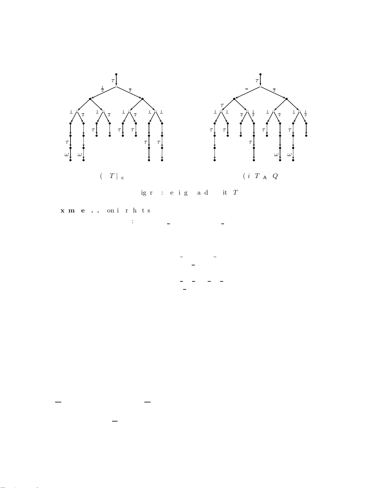
Logical Methods in Computer Science V ol. 4 (4:4) 2008, pp. 1–33 www .lmcs-online.org Submitted Feb . 7, 2008 Published Oct. 28, 2008 CHARA CTERISING TESTING PREORDERS F OR FINIT E PR OBABILISTIC PR OC ESSES ∗ YUXIN DENG a , ROB V AN GLABBEEK b , MA TTHEW HENN ESSY c , AND CAR ROLL MORG AN d a Shanghai Jiao T ong Universit y , China, and Universit y of New South W ales, A ustralia e-mail addr ess : yuxindeng@sjtu.edu.cn b National ICT Australia, and Un ivers ity of New South W ales , Australia e-mail addr ess : rvg@cs.stanford.edu c T rinit y College Dub lin, Ireland e-mail addr ess : matthew.hennessy@cs.tcd.ie d Universit y of New South W ales, Australia e-mail addr ess : carrollm@cse. unsw.edu.au Abstra ct. In 1992 W ang & Larsen extended the ma y- and must preorders of De Nicola and Hennessy to pro cesses featuring probabilistic as w ell as nond eterministic c hoice. They concluded with tw o p roblems that ha ve remained op en throughout the years, n amely to ﬁnd complete axiomatisatio ns and alternativ e characterisa tions for these preorders. This pap er solves b oth problems for ﬁn ite pro cesses with silent move s. It characterises the may preorder in terms of simulatio n, and the m ust preorder in terms of failure sim ulation. It also giv es a c haracterisatio n of b oth preorders using a modal logi c. Finally it axiomatises b oth preorders ov er a probabilistic vers ion of ﬁnite CSP . 1. Introduction A satisfac tory semanti c theory for pro cesses w hic h encompass b oth n ondeterministic and probabilistic b ehaviour has b ee n a long-sta nding researc h problem [13, 41, 28 , 20, 38, 39, 36, 22, 32, 37, 14, 26, 31, 1, 23, 29, 3, 40, 7]. In 1992 W ang & Larsen p o sed the problems of ﬁnding complete axiomatisat ions and alternativ e c haracterisatio ns for a natural gener- alisatio n o f the standard testing preorders [6] to suc h processes [41]. Here w e solv e both problems, at least for ﬁnite pro cesses, b y pro viding a detailed accoun t of b ot h ma y- and 1998 ACM Subje ct Classiﬁc ation: F.3.2, D.3.1. Key wor ds and phr ases: Probabilistic pro cesses, testing semantics, sim ulation, axiomatisatio n. ∗ An ext en ded abstract of t his pap er has app eared as [9]. a,c,d Deng wa s supp orted by th e National N atural Science F oundation of China (60703033) and the ARC (DP034557 ). Hennessy w ould lik e t o ac know ledge th e supp ort of SFI and The Roy al So ciet y , UK. Morgan w ould like to ackno wledge the supp ort of the Australian Researc h Council (ARC) Gran t DP034557. LOGICAL METHODS l IN COMPUTER SCIENCE DOI:10.216 8/LMCS-4 (4:4) 2008 c  Y . Den g, R. van Glabbeek, M . Henness y, and C . Morgan CC  Crea tive Commons 2 Y. DENG, R. V AN GLABBEEK, M. HENNESSY, AND C. MORG AN m ust testing preorders for a ﬁnite v ersion of the pro cess calculus CSP extended with pr ob- abilistic c hoice. F or eac h preorder we pro vide thr ee indep end en t charact erisations, using (i) co-inductiv e sim ulation r elations, (ii) a mo d al logic and (iii) sets of inequations. T esting pro c esses: Ou r starting p oint is the ﬁnite pro cess calculus pCSP [8] obtained b y adding a probabilistic c hoice op erat or to ﬁnite C S P; like others who ha v e done the same, w e now hav e thr e e c hoice op erat ors, external P  Q , inte rnal P ⊓ Q and the newly added probabilistic c hoice P p ⊕ Q . S o a seman tic theory for pCSP will h av e to pro vide a coheren t accoun t of the p recise relationships b et w een these op erators. As a ﬁrst step, in Section 2 we provide an inte rpretation of pCSP as a pr ob abilistic lab el le d tr ansition system , in which, follo wing [38 , 20], state-to -state transitions lik e s α − → s ′ from standard lab elled transition systems are generalised to the form s α − → ∆, where ∆ is a distribution , a mapping assigning pr obab ilities to states. W ith this in terpretation we obtain in Section 3 a v ersion of the testing preorders of [6] for pCSP p ro cesses, ⊑ pma y and ⊑ pmu st . T hese are based on the abilit y of pro cesses to p ass tests ; the tests we use are simply pCSP p ro cesses in wh ic h certain states are mark ed as suc c ess states . See [8] for a detailed discussion of the p o w er of suc h tests. The ob ject of this pap er is to giv e alternativ e c haracterisati ons of these testing pr e- orders. Th is problem w as addr essed previously b y Segala in [37 ], b u t using testing preorders ( b ⊑ Ω pma y and b ⊑ Ω pmu st ) that diﬀer in t w o w a ys fr om the ones in [6, 15, 41, 8] and the p resen t pap er. First of all, in [37] the success of a test is ac hiev ed by the actual exe cution of a predeﬁned suc c ess action , rather than the reac h ing of a su ccess state. W e call this an ac- tion -based approac h, as opp osed to the state -based appr oac h used in th is p ap er. Secondly , [37] employs a count able num b er of su ccess actions instead of a single one; w e call this ve ctor-b ase d , as opp osed to sc alar , testing. S egala’ s results in [37] dep e nd crucially on this form of testing. T o ac hiev e our current results, we need Segala’s preorders as a stepping stone. W e relate them to ours b y considering inte rmediate preorders b ⊑ pma y and b ⊑ pmu st that arise from actio n-based b u t s calar testing, and use a recen t result [10] sayi ng that for ﬁnite pro cesses the pr eorders b ⊑ Ω pma y and b ⊑ Ω pmu st coincide with b ⊑ pma y and b ⊑ pmu st . Here we show that on pCS P the pr eorders b ⊑ pma y and b ⊑ pmu st also coincide with ⊑ pma y and ⊑ pmu st . 1 Sim ula t ion preorders: In Section 4 w e use the transitions s α − → ∆ to d eﬁne t wo co- inductiv e preorders, the simulat ion preorder ⊑ S [36, 29, 8], and the n ov el f ailur e simulation preorder ⊑ FS o ver pCSP pro cesses. The latter extends the failure simulati on preorder of [11] to probabilistic pro cesses. Th eir d eﬁnition u ses a natural generalisation of the transitions, ﬁrst (Kleisli-st yle) to tak e the form ∆ α − → ∆ ′ , and then to we ak versio ns ∆ α = ⇒ ∆ ′ . The second p r eorder diﬀers from the ﬁrst one in the use of a failur e predicate s X − 6 → , indicating that in the state s none of the actions in X can b e p erf orm ed. Both preorders are pr eserv ed b y all the op erators in pCSP , and are sound with resp ect to the testing pr eorders; that is P ⊑ S Q imp lies P ⊑ pma y Q and P ⊑ FS Q imp lies P ⊑ pmu st Q . F or ⊑ S this w as established in [8], and here w e use similar tec hn iques in the pro ofs for ⊑ FS . But c ompleteness , that the testing preorders imply the r esp ectiv e sim u lation p r eorders, requires some ingen uit y . W e prov e it indirectly , inv olving a charact erisation of the testing and simulat ion preorders in terms of a mo d al logic. 1 How ever in the presence of divergence they are sligh tly diﬀerent. CHARACTERISI NG T ESTING PREOR D ERS FOR FINITE PROBABILISTIC PROCESSES 3 Mo dal logic: Our mo dal logic, deﬁn ed in Section 7, uses ﬁ nite conjunction V i ∈ I ϕ i , the mo dalit y h a i ϕ from the Hennessy-Milner Logic [16], and a no v el probabilistic construct L i ∈ I p i · ϕ i . A satisfaction relatio n b et w een pro cesses and formulae then giv es, in a natural manner, a lo gic al pr e or der b et w een pro cesses: P ⊑ L Q means that eve ry L -form ula satisﬁed b y P is also satisﬁed by Q . W e establish that ⊑ L coincides w ith ⊑ S and ⊑ pma y . T o capture failures, we add, for ev ery set of actions X , a formula ref ( X ) to our logic, satisﬁed by any pr o cess which, after it can do no further in ternal actions, can p erform none of the actions in X either. The constructs V , h a i an d ref () stem from the mo dal c h aracterisati on of the non-probabilistic failure sim ulation preorder, give n in [11]. W e sho w that ⊑ pmu st , as well as ⊑ FS , can b e c haracterised in a similar manner with th is extended mo dal logic. Pro of strategy: W e p ro v e these c haracterisati on results thr ough t wo cycles of inclusions: ⊑ L ⊆ ⊑ S [8] ⊆ ⊑ pma y ⊆ b ⊑ pma y [10] = b ⊑ Ω pma y ⊆ ⊑ L ⊑ F ⊆ ⊑ FS ⊆ ⊑ pmu st ⊆ b ⊑ pmu st [10] = b ⊑ Ω pmu st ⊆ ⊑ F | {z } | {z } | {z } | {z } | {z } | {z } Sec. 7 Sec. 4 Sec. 3 Sec. 5 Sec. 6 Sec. 8 In Section 7 w e sho w that P ⊑ L Q imp lies P ⊑ S Q (and hence P ⊑ pma y Q ), and lik ewise for ⊑ F and ⊑ FS ; the pro of in v olv es constructing, for eac h pCSP pro cess P , a char acteristic formula ϕ P . T o obtain the other direction, in S ection 8 we s ho w how ev ery mo dal formula ϕ can b e captured , in some sense, b y a test T ϕ ; essential ly the abilit y of a pCS P pr o cess to satisfy ϕ is determined by its abilit y to pass the test T ϕ . W e capture the conjunction of t wo form ulae b y a p robabilistic c h oice b et ween the corresp onding tests; in order to preve nt the results f rom these tests getting mixed up, we employ the ve ctor-based tests of [37], so that we can use diﬀerent success actions in the s eparate p r obabilistic branches. Therefore, w e complete our p r o of by d emonstrating that the state-based testing pr eorders imp ly the action-based ones (Section 5) and recalling th e resu lt from [10 ] that the action-based scalar testing preorders imply the vect or-based ones (Section 6). (In)equations: It is well-kno wn that ma y- and must testing for standard CSP can b e captured equationally [6, 2, 15]. In [8] w e s ho w ed that most of the standard equations are n o longer v alid in the probabilistic setting of pCSP ; we also pro vided a set of axioms whic h are complete with resp ect to (probabilistic) ma y-testing for the sub-language of pCSP without probabilistic c h oice. Here we extend this result, b y sho wing, in Section 10 , that b oth P ⊑ pma y Q and P ⊑ pmu st Q can still b e captured equationally o v er fu ll pCSP . I n the ma y case the essenti al (in)equation r equired is a. ( P p ⊕ Q ) ⊑ a.P p ⊕ a.Q The m ust case is more in volv ed: in the absence of the distributivit y of the external and in- ternal c hoices o v er eac h other, to obtain complete ness w e require a complicated inequational sc h ema. 4 Y. DENG, R. V AN GLABBEEK, M. HENNESSY, AND C. MORG AN 2. Finite p robabilistic CSP Let Act b e a ﬁnite set of visible (or external ) actions, ranged o ver b y a, b, · · · , which pro cesses can p erform. Then th e ﬁ nite p robabilistic CS P pro cesses are giv en b y the follo w ing t w o- sorted synta x: P ::= S | P p ⊕ P S ::= 0 | a.P | P ⊓ P | S  S | S | A S W e write pCSP , ranged o v er by P, Q , for the set of pro cess terms deﬁned by this grammar, and sCSP , ranged o v er by s, t , for the subs et comprising only the state -based pro cess terms (the sub -sort S ab o v e). The pro cess P p ⊕ Q , for 0 < p < 1, repr esents a pr ob abilistic choic e b et w een P and Q : with probabilit y p it w ill act like P and with probabilit y 1 − p it w ill act lik e Q . Any pro cess is a probabilistic com bin ation of state-based pro cesses bu ilt by rep eated applicatio n of the op erator p ⊕ . Th e state-based p ro cesses hav e a CSP-lik e syn tax, inv olving the s topp ed pro cess 0 , action p reﬁxing a. for a ∈ Act , internal- and external choic es ⊓ and  , and a p ar al lel c omp osition | A for A ⊆ A ct . The pro cess P ⊓ Q will ﬁrst d o a so-called internal action τ 6∈ Act , c ho osing nondeter- ministic al ly b et we en P and Q . Th erefore ⊓ , lik e a. , acts as a gu ar d , in the sense that it con verts any pro cess argument s in to a state-based p ro cess. The pro cess s  t on the other hand do es n ot p erform actio ns itself, bu t merely allo ws its argument s to pro ceed, disabling one argument as so on as the other has d one a visible action. In order for this pro cess to start from a state rather than a probabilit y distribu tion of states, we require its argument s to b e state-based as w ell; the same app lies to | A . Finally , the expr ession s | A t , wh ere A ⊆ Act , represen ts p ro cesses s and t running in parallel. T hey ma y synchronise by p erform in g the same action from A sim u ltaneously; such a synchronisatio n results in τ . In addition s and t may in dep end ently do any action fr om ( Act \ A ) ∪ { τ } . Although formally the op erators  and | A can only b e applied to state-based pro cesses, informally we u se expressions of the form P  Q and P | A Q , w h ere P and Q are not state-based, as synta ctic sugar f or expressions in the ab o v e syn tax obtained by distributing  and | A o ver p ⊕ . Thus for example s  ( t 1 p ⊕ t 2 ) abb r eviates the term ( s  t 1 ) p ⊕ ( s  t 2 ). The full language of CSP [2, 17, 34] has many more op erators; we hav e simply c hosen a rep r esen tativ e selectio n, and ha ve added p r obabilistic c hoice. Ou r parallel op erator is not a CSP pr imitiv e, but it can easily b e expressed in terms of them—in particular P | A Q = ( P k A Q ) \ A , w h ere k A and \ A are the parallel comp osition and hiding op erators of [34]. It can also b e expressed in terms of the parallel comp osition, ren amin g and r estriction op erators of CCS. W e ha v e c hosen this (non-asso ciativ e) op erator for con v enience in deﬁn ing the application of tests to pro cesses. As usual we ma y elide 0 ; the p reﬁxing op erator a. binds stronger than any binary op erator; and precedence b et w een binary op erators is indicated via brac kets or spacing. W e will also sometimes u se indexed binary op erators, suc h as L i ∈ I p i · P i with P i ∈ I p i = 1 and all p i > 0, and e i ∈ I P i , for some ﬁnite ind ex set I . CHARACTERISI NG T ESTING PREOR D ERS FOR FINITE PROBABILISTIC PROCESSES 5 The ab o ve in tuitions are formalised b y an op er ational semantics 2 asso ciating with eac h pro cess term a graph-like stru cture represen ting its p ossible reactions to users’ r equ ests: w e use a generalisati on of lab elled transition systems [30] that includes probabilities. A (discrete) pr ob ability d istribution o v er a set S is a function ∆ : S → [0 , 1] with P s ∈ S ∆( s ) = 1; the supp ort of ∆ is giv en by ⌈ ∆ ⌉ = { s ∈ S | ∆ ( s ) > 0 } . W e write D ( S ), ranged o v er b y ∆ , Θ , Φ , for the set of all d istributions o v er S with ﬁn ite sup p ort; these ﬁn ite distributions are suﬃcient for the r esults of this pap er. W e also write s to denote the p oin t distribution assigning probabilit y 1 to s and 0 to all others, so that ⌈ s ⌉ = { s } . If p i ≥ 0 and ∆ i is a distribution for eac h i in some ﬁnite index set I , and P i ∈ I p i = 1, then the probabilit y distrib u tion P i ∈ I p i · ∆ i ∈ D ( S ) is giv en b y ( X i ∈ I p i · ∆ i )( s ) = X i ∈ I p i · ∆ i ( s ) ; w e will sometimes wr ite it as p 1 · ∆ 1 + . . . + p n · ∆ n when the index set I is { 1 , . . . , n } . F or ∆ a distribu tion o v er S and function f : S → X in to a ve ctor space X w e sometimes write Exp ∆ ( f ) for P s ∈ S ∆( s ) · f ( s ), the exp e cte d value of f . Our primary use of this notation is with X b eing the v ector space of r eals or tuples of reals. More generally , for fun ction F : S → P + ( X ) with P + ( X ) b eing the collectio n of non-empty sub sets of X , w e deﬁn e Exp ∆ F := { Exp ∆ ( f ) | f ∈ F } ; h ere f ∈ F means that f : S → X is a choic e function for F , that is it satisﬁes the constrain t that f ( s ) ∈ F ( s ) f or all s ∈ S . W e no w giv e the prob abilistic generalisati on of lab elled transition systems (L TSs): Deﬁnition 2.1. A pr ob abilistic lab el le d tr ansition system (pL TS) 3 is a triple h S, L, →i , where (i) S is a set of states, (ii) L is a set of trans ition lab els, (iii) relation → is a subset of S × L × D ( S ). As with L TSs, we u s ually write s α − → ∆ for ( s, α, ∆) ∈ → , s α − → for ∃ ∆ : s α − → ∆ and s → for ∃ α : s α − → . An L TS ma y b e viewed as a d egenerate pL TS, one in which only p oin t distributions are u sed. The op erational semant ics of pCSP is deﬁn ed by a particular pL TS h sCSP , Act τ , →i , con- structed by taking sCS P to b e th e set of states an d Act τ := Act ∪ { τ } the set of transition lab els; w e let a range o v er Act and α ov er Act τ . W e int erpret pCSP p ro cesses P as distri- butions [ P ℄ ∈ D ( sCSP ) via the fun ction [ ℄ : pCSP → D ( sCSP ) deﬁned b elo w: [ s ℄ := s f or s ∈ sCSP [ P p ⊕ Q ℄ := p · [ P ℄ + (1 − p ) · [ Q ℄ . Note that for eac h P ∈ pCSP the distribution [ P ℄ is ﬁnite, that is it has ﬁnite supp ort. The deﬁnition of the relations α − → is giv en in Figure 1. These ru les are v ery similar to the standard ones used to interpret CSP as an L TS [34], bu t mo diﬁed so that the result of an actio n is a distribution. The r u les for external choice and parallel comp osition use 2 Although the sy ntax of pCSP is similar to other probabilistic extensions of CSP [28, 32, 31], our semantics diﬀers. F or more d etailed comparisons, see Section 12. 3 Essen tially the same mo del has app eared in the literature under diﬀerent names such as NP-systems [20], pr ob abilistic pr o c esses [22], sim pl e pr ob abilistic automata [36], pr ob abil istic tr ansition systems [23] etc. F urthermore, th ere are strong structural similaritie s with Markov De cision Pr o c esses [35, 10]. 6 Y. DENG, R. V AN GLABBEEK, M. HENNESSY, AND C. MORG AN a.P a − → [ P ℄ P ⊓ Q τ − → [ P ℄ P ⊓ Q τ − → [ Q ℄ s 1 a − → ∆ s 1  s 2 a − → ∆ s 2 a − → ∆ s 1  s 2 a − → ∆ s 1 τ − → ∆ s 1  s 2 τ − → ∆  s 2 s 2 τ − → ∆ s 1  s 2 τ − → s 1  ∆ s 1 α − → ∆ α 6∈ A s 1 | A s 2 α − → ∆ | A s 2 s 2 α − → ∆ α 6∈ A s 1 | A s 2 α − → s 1 | A ∆ s 1 a − → ∆ 1 , s 2 a − → ∆ 2 a ∈ A s 1 | A s 2 τ − → ∆ 1 | A ∆ 2 Figure 1: Op erational seman tics of pCSP an obvio us notation for distributing an op erator o v er a distribution; for example ∆  s represen ts the distribution give n by (∆  s )( t ) = ( ∆( s ′ ) if t = s ′  s 0 otherwise . W e sometimes write τ .P for P ⊓ P , thus giving τ .P τ − → [ P ℄ . W e graphically d ep ict the op erational semantic s of a pCSP expression P b y dra wing the part of the pL T S deﬁned ab o v e that is reac hable f r om [ P ℄ as a ﬁnite acyclic directed graph, often unw ound int o a tree. States are represent ed b y no des of the form • and distribu tions b y no des of the form ◦ . F or an y state s and d istribution ∆ with s α − → ∆ we dra w an edge from s to ∆, lab elled with α . F or an y distribution ∆ and state s in ⌈ ∆ ⌉ , th e supp ort of ∆, w e dr a w an edge from ∆ to s , lab elled w ith ∆( s ). Example 2.2. C onsider the tw o pr o cesses P := a. (( b.d  c.e ) 1 2 ⊕ ( b.f  c.g )) Q := a. (( b.d  c.g ) 1 2 ⊕ ( b.f  c.e )) . Their tree representa tions are depicted in Figure 2 (i) and (ii). T o make these trees m ore compact we omit no d es ◦ wh en they repr esen t trivial p oin t distribu tions. 3. Testing pCSP processes A test is a pCSP process except that it may ha v e subterms ω .P for fresh ω 6∈ Act τ , a sp ecial action rep orting success; w e write pCSP ω for the set of all tests, and sCSP ω for th e subs et of state-based p ro cess terms that may inv olv e th e action ω , and the op erational semant ics ab o v e is extended by treati ng ω lik e any other action from Act . T o apply test T to pr o cess P w e form the pro cess T | Act P in which al l visible actions of P must synchronise with T , and d eﬁne a set of testing outcomes A ( T , P ) where eac h outcome, in [0 , 1], arises from a resolution of the nond eterministic choic es in T | Act P and giv es the probabilit y that this resolution will reac h a suc c ess state , one in w hic h ω is p ossible. CHARACTERISI NG T ESTING PREOR D ERS FOR FINITE PROBABILISTIC PROCESSES 7 b b c a b 1 2 b b b d b c b e b 1 2 b b b f b c b g b b c a b 1 2 b b b d b c b g b 1 2 b b b f b c b e b b a b c τ b 1 2 b b b d b ω b 1 2 b c b e b ω b c τ b 1 2 b b b f b ω b 1 2 b c b g b ω ( i ) P ( ii ) Q ( iii ) T Figure 2: Example pro cesses P , Q and test T T o this end , we ind u ctiv ely deﬁne a r esults-gathering fu nction V : sCSP ω → P + ([0 , 1]) ; it extends to t yp e D ( sCSP ω ) → P + ([0 , 1]) via the conv ent ion V (∆) := Exp ∆ V . V ( s ) :=      { 1 } if s ω − → , S { V (∆) | s α − → ∆ } if s ω − 6 → but still s → , { 0 } if s 6→ In the ﬁrst case ab o v e s ω − → signiﬁes that s is a s u ccess state. In the second case w e mean that ω is not p ossible from s —hence s is n ot a success state—but that at least one “non- success” action α ∈ A ct τ is—and p ossibly seve ral—and then th e union is o v er all suc h α . This is done s o that V accoun ts for su ccess actions in pr o cesses generally; wh en applied to test outcomes, how ev er, the only n on-success action is τ . Note that V is well deﬁned when applied to ﬁ nite, lo op-free pro cesses, su c h as the ones of pCS P . Deﬁnition 3.1. F or any pCSP pro cess P and test T , deﬁne A ( T , P ) := V [ T | Act P ℄ . With this deﬁnition, the general testing f r amew ork of [6] yields t w o testing preorders for pCSP , one based on may testing, written P ⊑ pma y Q , and the other on must testing, w ritten P ⊑ pmu st Q . Deﬁnition 3.2. Th e may- and must preorders are giv en b y P ⊑ pma y Q iﬀ for all tests T : A ( T , P ) ≤ Ho A ( T , Q ) P ⊑ pmu st Q iﬀ for all tests T : A ( T , P ) ≤ Sm A ( T , Q ) with ≤ Ho , ≤ Sm the Hoare, S m yth pr eorders on P + [0 , 1]. These are deﬁned as follo ws : X ≤ Ho Y iﬀ ∀ x ∈ X : ∃ y ∈ Y : x ≤ y X ≤ Sm Y iﬀ ∀ y ∈ Y : ∃ x ∈ X : x ≤ y In other wo rds, Q is a correct reﬁn emen t of P i n the probabilistic may-t esting p reorder if eac h outcome (in [0,1] ) of applying a test to pro cess P can b e matc hed or increased b y applying the same test to p ro cess Q . Like wise, Q is a correct r eﬁnemen t of P in the probabilistic m u s t-testing preorder if eac h outcome of applying a test to Q matc hes or increases an outcome obtainable by applying th e same test to P . 8 Y. DENG, R. V AN GLABBEEK, M. HENNESSY, AND C. MORG AN b b c τ b 1 2 b c τ b 1 2 b τ b τ b ω b 1 2 b τ b τ b ω b c τ b 1 2 b τ b 1 2 b τ b 1 2 b c τ b 1 2 b τ b 1 2 b τ b c τ b 1 2 b τ b τ b ω b 1 2 b τ b τ b ω b b c τ b 1 2 b c τ b 1 2 b τ b τ b ω b 1 2 b τ b c τ b 1 2 b τ b 1 2 b τ b τ b ω b 1 2 b c τ b 1 2 b τ b 1 2 b τ b τ b ω b c τ b 1 2 b τ b τ b ω b 1 2 b τ ( i ) T | Act P ( ii ) T | Act Q Figure 3: T esting P and Q with T . Example 3.3. C onsider the test T := a. (( b.d.ω 1 2 ⊕ c.e.ω ) ⊓ ( b.f .ω 1 2 ⊕ c.g.ω )) whic h is graphicall y depicted in Figure 2 (iii). If w e apply T to p ro cesses P and Q giv en in Example 2.2 , we form the tw o pr o cesses describ ed in Figure 3. It is then easy to calculate the testing outcomes: A ( T , P ) = 1 2 · { 1 , 0 } + 1 2 · { 1 , 0 } = { 0 , 1 2 , 1 } A ( T , Q ) = 1 2 · { 1 2 } + 1 2 · { 1 2 } = { 1 2 } . W e can see that P and Q can b e distinguished b y the test T since A ( T , P ) 6≤ Ho A ( T , Q ) and A ( T , Q ) 6≤ Sm A ( T , P ). In other words, we hav e P 6⊑ pma y Q and Q 6⊑ pmu st P b ecause of the witness test T . In [8] w e applied the testing framew ork describ ed ab ov e to sh ow th at many standard laws of CSP are no longer v alid in the probabilistic setting of pCSP , and to pro vide coun terexamples for a few d istributiv e la w s in v olving probabilistic c h oice that ma y app ear plausible at ﬁrst sigh t. W e also sho wed that P ⊑ pmu st Q implies Q ⊑ pma y P for all pCSP pro cesses P and Q , i.e. that m ust testing is more discriminating than ma y testing and that the pr eorders ⊑ pma y and ⊑ pmu st are orient ed in opp osite directions. 4. Simula tion and f ailur e simula tion Let R ⊆ S × D ( S ) b e a relation from states to distributions. As in [8], w e lift it to a relatio n R ⊆ D ( S ) ×D ( S ) by lett ing ∆ R Θ w h enev er there is a ﬁ nite index set I and p ∈ D ( I ) suc h that (i) ∆ = P i ∈ I p i · s i , (ii) F or eac h i ∈ I there is a distribution Φ i s.t. s i R Φ i , (iii) Θ = P i ∈ I p i · Φ i . CHARACTERISI NG T ESTING PREOR D ERS FOR FINITE PROBABILISTIC PROCESSES 9 F or fun ctions, th e lifting op eration can b e understo o d as a Kleisli construction on a pr ob a- bilistic p ow er d omain [18], and w as implicit in the wo rk of Kozen [25]; in ou r more general setting of relations, it can equiv alentl y b e d eﬁned in terms of a distribution on R , some- times called weight function (see e.g. [21, 36]). An imp ortant p oint here is that in the decomp osition (i) of ∆ 1 in to P i ∈ I p i · s i , the states s i are not ne c essarily distinct : that is, the decomp osition is not in general u nique. F or notational con venience, the lifted v ersions of the transition relations α − → f or α ∈ A ct τ are again d enoted α − → . W e wr ite s ˆ τ − → ∆ if either s τ − → ∆ or ∆ = s ; again ∆ 1 ˆ τ − → ∆ 2 denotes the lifted relation. Thus for example we ha v e [ ( a ⊓ b ) 1 2 ⊕ ( a ⊓ c ) ℄ ˆ τ − → [ a 1 2 ⊕ (( a ⊓ b ) 1 2 ⊕ c ) ℄ b ecause (i) [ ( a ⊓ b ) 1 2 ⊕ ( a ⊓ c ) ℄ = 1 4 · [ ( a ⊓ b ) ℄ + 1 4 · [ ( a ⊓ b ) ℄ + 1 4 · [ ( a ⊓ c ) ℄ + 1 4 · [ ( a ⊓ c ) ℄ , (ii) [ ( a ⊓ b ) ℄ τ − → [ a ℄ [ ( a ⊓ b ) ℄ ˆ τ − → [ a ⊓ b ℄ [ ( a ⊓ c ) ℄ τ − → [ a ℄ [ ( a ⊓ c ) ℄ τ − → [ c ℄ (iii) and [ a 1 2 ⊕ (( a ⊓ b ) 1 2 ⊕ c ) ℄ = 1 4 · [ a ℄ + 1 4 · [ ( a ⊓ b ) ℄ + 1 4 · [ a ℄ + 1 4 · [ c ℄ . W e now deﬁn e the weak transition r elatio n ˆ τ = ⇒ as the transitiv e and reﬂexiv e closure ˆ τ − → ∗ of ˆ τ − → , while for a 6 = τ we let ∆ 1 ˆ a = ⇒ ∆ 2 denote ∆ 1 ˆ τ = ⇒ a − → ˆ τ = ⇒ ∆ 2 . Finally , we write s X − 6 → with X ⊆ Act when ∀ α ∈ X ∪ { τ } : s α − 6 → , and ∆ X − 6 → when ∀ s ∈ ⌈ ∆ ⌉ : s X − 6 → . The main prop erties of the lifted w eak transition relations whic h are used throughout the pap er are giv en in the follo win g lemma. Lemma 4.1. Supp ose P i ∈ I p i = 1 and ∆ i ˆ α = ⇒ Φ i for e ach i ∈ I , with I a ﬁnite index set. Then X i ∈ I p i · ∆ i ˆ α = ⇒ X i ∈ I p i · Φ i . Conversely, if P i ∈ I p i · ∆ i ˆ α = ⇒ Φ then Φ = P i ∈ I p i · Φ i for some Φ i such that ∆ i ˆ α = ⇒ Φ i for e ach i ∈ I . Pr o of. T he ﬁrst claim occurs as Lemma 6.6 of [8]. T h e second follo ws by rep eated applica- tion of Pr op osition 6.1(ii) of [8], taking R to b e ˆ τ − → and a − → f or a ∈ Act . Deﬁnition 4.2. A r elation R ⊆ sCSP × D ( sCS P ) is said to b e a failur e simulation if for all s, Θ , α, ∆ , X w e hav e that • s R Θ ∧ s α − → ∆ implies ∃ Θ ′ : Θ ˆ α = ⇒ Θ ′ ∧ ∆ R Θ ′ • s R Θ ∧ s X − 6 → implies ∃ Θ ′ : Θ ˆ τ = ⇒ Θ ′ ∧ Θ ′ X − 6 → . W e write s ⊳ FS Θ to mean th at there is some failure sim ulation R such that s R Θ. Similarly , we deﬁne simulation 4 and s ⊳ S Θ by dr opp ing the second clause in Deﬁnition 4.2. 5 Deﬁnition 4.3. The simulation pr e or der ⊑ S and failur e simulation pr e or der ⊑ FS on pCSP are deﬁn ed as follo ws: P ⊑ S Q iﬀ [ Q ℄ ˆ τ = ⇒ Θ for some Θ with [ P ℄ ⊳ S Θ P ⊑ FS Q iﬀ [ P ℄ ˆ τ = ⇒ Θ for some Θ with [ Q ℄ ⊳ FS Θ . (Note the opp osing dir ections.) The equiv alences generated by ⊑ S and ⊑ FS are called (failur e) simulation e quiv alenc e , denoted ≃ S and ≃ FS , resp ectiv ely . 4 It is called f orwar d simulation in [36]. 5 W e have reversed the orienta tion of the sy mbols ⊲ S and ⊲ FS w.r.t. [8] and [9]; the p oin ty side now p oints to a single state, and the ﬂat side to a distribution. 10 Y. DENG, R. V AN GLABBEEK, M. HENNESSY, AND C. MORG AN Example 4.4. Compare the pro cesses P = a 1 2 ⊕ b and P ⊓ P . Note that [ P ℄ is th e distribution 1 2 · a + 1 2 · b whereas [ P ⊓ P ℄ is the p oint distribution P ⊓ P . Th e relation R giv en by ( P ⊓ P ) R ( 1 2 · a + 1 2 · b ) a R a b R b 0 R 0 is a sim ulation, b ecause the τ -step P ⊓ P τ − → ( 1 2 · a + 1 2 · b ) can b e matc hed by the idle transition ( 1 2 · a + 1 2 · b ) ˆ τ = ⇒ ( 1 2 · a + 1 2 · b ), and we ha v e ( 1 2 · a + 1 2 · b ) R ( 1 2 · a + 1 2 · b ). Th us ( P ⊓ P ) ⊳ S ( 1 2 · a + 1 2 · b ) = [ P ℄ , hence [ P ⊓ P ℄ ⊳ S [ P ℄ , and therefore P ⊓ P ⊑ S P . This t yp e of reasoning d o es n ot ap p ly to the other direction. An y simula tion R with ( 1 2 · a + 1 2 · b ) R P ⊓ P would ha v e to satisfy a R P ⊓ P and b R P ⊓ P . Ho w ev er, the mo v e a a − → 0 cannot b e matc hed by the pro cess P ⊓ P , as the only transition the latt er pro cess can do is P ⊓ P τ − → ( 1 2 · a + 1 2 · b ), and only half of that distribution can m atc h th e a -mo ve. T hus, no suc h sim u lation exists, and w e ﬁnd [ P ℄ 6 ⊳ S [ P ⊓ P ℄ . Neve rtheless, we still ha v e P ⊑ S P ⊓ P . Here, the transition ˆ τ = ⇒ from Deﬁnition 4.3 comes to the rescue. As [ P ⊓ P ℄ ˆ τ = ⇒ [ P ℄ and [ P ℄ ⊳ S [ P ℄ , we obtain P ⊑ S P ⊓ P . Example 4.5. Let P = a 1 2 ⊕ b and Q = P  P . W e ha v e P ⊑ S Q b ecause [ P ℄ ⊳ S [ Q ℄ whic h comes from the follo win g observ ations: (1) [ P ℄ = 1 2 · a + 1 2 · b (2) [ Q ℄ = 1 2 · ( 1 2 · a  a + 1 2 · a  b ) + 1 2 · ( 1 2 · b  a + 1 2 · b  b ) (3) a ⊳ S ( 1 2 · a  a + 1 2 · a  b ) (4) b ⊳ S ( 1 2 · b  a + 1 2 · b  b ) This kind of reasoning d o es n ot apply to ⊳ FS . F or example, we h a v e a 6 ⊳ FS ( 1 2 · a  a + 1 2 · a  b ) b ecause th e state on th e left hand side can r efuse to do action b while the distribution on the right hand side cannot. Indeed, it holds that Q 6⊑ FS P . W e ha v e already sho w n in [8] that ⊑ S is a precongruence and that it implies ⊑ pma y . Similar results can b e established f or ⊑ FS as well. Belo w we summarise these facts. Prop osition 4.6. Supp ose ⊑ ∈ {⊑ S , ⊑ FS } . Then ⊑ is a pr e or der, and if P i ⊑ Q i for i = 1 , 2 then a.P 1 ⊑ a.Q 1 for a ∈ Act and P 1 ⊙ P 2 ⊑ Q 1 ⊙ Q 2 for ⊙ ∈ {⊓ ,  , p ⊕ , | A } . Pr o of. T he case ⊑ S w as pro ved in [8 , Corollary 6.10 and Theorem 6.13]; th e case ⊑ FS is analogous. As an example, w e sh o w that ⊑ FS is preserved und er parallel comp osition. The k ey step is to sho w that the b inary relation R ⊆ sCSP × D ( sCSP ) deﬁned by R := { ( s 1 | A s 2 , ∆ 1 | A ∆ 2 ) | s 1 ⊳ FS ∆ 1 ∧ s 2 ⊳ FS ∆ 2 } . is a f ailure simulati on. Supp ose s i ⊳ FS ∆ i for i = 1 , 2 and s 1 | A s 2 X − 6 → for some X ⊆ Act . F or eac h a ∈ X there are tw o p ossibilities: • If a 6∈ A then s 1 a − 6 → and s 2 a − 6 → , since otherwise we wo uld h a ve s 1 | A s 2 a − → . • If a ∈ A then either s 1 a − 6 → or s 2 a − 6 → , since otherwise we would ha v e s 1 | A s 2 τ − → . Hence we can partition the set X in to three subs ets: X 0 , X 1 and X 2 suc h that X 0 = X \ A and X 1 ∪ X 2 ⊆ A with s 1 X 1 − − 6 → and s 2 X 2 − − 6 → , but allo wing s 1 a − 6 → for some a ∈ X 2 and s 2 a − 6 → for some a ∈ X 1 . W e th en ha v e th at s i X 0 ∪ X i − − − − 6 → for i = 1 , 2. By the assumption that s i ⊳ FS ∆ i for i = 1 , 2, there is a ∆ ′ i with ∆ i ˆ τ = ⇒ ∆ ′ i X 0 ∪ X i − − − − 6 → . Th erefore ∆ ′ 1 | A ∆ ′ 2 X − 6 → as w ell. It is stated in [8, Lemma 6.12(i)] that if Φ ˆ τ = ⇒ Φ ′ then Φ | A ∆ ˆ τ = ⇒ Φ ′ | A ∆ and CHARACTERISI NG T ESTING PREOR D ERS FOR FINITE PROBABILISTIC PROCESSES 11 ∆ | A Φ ˆ τ = ⇒ ∆ | A Φ ′ . So w e h a ve ∆ 1 | A ∆ 2 ˆ τ = ⇒ ∆ ′ 1 | A ∆ ′ 2 . Hence ∆ 1 | A ∆ 2 can matc h up the failures of s 1 | A s 2 . The matc hin g up of transitions and the using of R to p ro v e the preserv ation prop ert y of ⊑ FS under parallel comp osition are similar to those in the corresp onding pro of for sim- ulations [8, T heorem 6.13(v)], so we omit them. W e recall the follo wing r esult from [8, Theorem 6.17]. Theorem 4.7. If P ⊑ S Q then P ⊑ pma y Q . Pr o of. F or any test T ∈ pCSP ω and pr o cess P ∈ pCSP the set V ( T | Act P ) is ﬁnite, so P ⊑ pma y Q iﬀ max ( V ( [ T | Act P ℄ )) ≤ max ( V ( [ T | Act Q ℄ )) for every test T . (4.1) The follo wing prop erties for ∆ 1 , ∆ 2 ∈ pCSP ω and α ∈ Act τ are not h ard to establish: ∆ 1 ˆ α = ⇒ ∆ 2 implies max ( V (∆ 1 )) ≥ max ( V (∆ 2 )) . (4 .2) ∆ 1 ⊳ S ∆ 2 implies max ( V (∆ 1 )) ≤ max ( V (∆ 2 )) . (4.3) In [8, Lemma 6.15 and Prop osition 6.16] similar prop erties are pr o v en u sing a function maxlive instead of max ◦ V . T he same argumen ts apply h ere. No w s upp ose P ⊑ S Q . Since ⊑ S is pr eserved b y the parallel op erator w e hav e that T | Act P ⊑ S T | Act Q for an arbitrary test T . By deﬁn ition, this means that there is a distribution ∆ su ch that [ T | Act Q ℄ ˆ τ = ⇒ ∆ and [ T | Act P ℄ ⊳ S ∆. By (4.2) and (4.3) w e infer that max ( V ( [ T | Act P ℄ )) ≤ max ( V ( [ T | Act Q ℄ )). The result n o w follo w s from (4.1). It is tempting to use the same idea to pr o v e that ⊑ FS implies ⊑ pmu st , b ut no w using the function min ◦ V . Ho w ev er, the min -analogue of P r op ert y (4.2) is in general inv alid. F or example, let R b e the pro cess a | Act ( a  ω ). W e hav e min ( V ( R )) = 1, ye t R τ − → 0 | Act 0 and min ( V ( 0 | Act 0 )) = 0. Therefore, it is not the case th at ∆ 1 ˆ τ = ⇒ ∆ 2 implies min ( V (∆ 1 )) ≤ min ( V (∆ 2 )). Our strateg y is therefore as follo ws. W rite s α − → ω ∆ if b oth s ω − 6 → and s α − → ∆ hold. W e deﬁne ˆ τ − → ω as ˆ τ − → using τ − → ω in place of τ − → . Similarly w e deﬁne = ⇒ ω and ˆ α = ⇒ ω . Thus the subscript ω on a transition of any kin d indicates that no state is passed through in wh ich ω is en abled. A versio n of failure sim u lation adapted to these transition relatio ns is then deﬁned as follo ws. Deﬁnition 4.8. Let ⊳ e FS ⊆ sCSP ω × D ( sCSP ω ) b e the largest r elation su c h that s ⊳ e FS Θ implies • if s α − → ω ∆ then there is some Θ ′ with Θ ˆ α = ⇒ ω Θ ′ and ∆ ⊳ e FS Θ ′ • if s X − 6 → with ω ∈ X then there is some Θ ′ with Θ ˆ τ = ⇒ ω Θ ′ and Θ ′ X − → . Let P ⊑ e FS Q iﬀ [ P ℄ ˆ τ = ⇒ ω Θ for s ome Θ with [ Q ℄ ⊳ e FS Θ. Note that for p ro cesses P , Q in p CSP (as opp osed to pCSP ω ), we hav e P ⊑ FS Q iﬀ P ⊑ e FS Q . Prop osition 4.9. If P , Q ar e pr o c e sses in pCSP with P ⊑ FS Q and T is a pr o c ess in pCSP ω then T | Act P ⊑ e FS T | Act Q . Pr o of. S imilar to the pro of of Prop osition 4.6. 12 Y. DENG, R. V AN GLABBEEK, M. HENNESSY, AND C. MORG AN Prop osition 4.10. The fol lowing pr op erties hold for min ◦ V , with ∆ 1 , ∆ 2 ∈ D ( sCSP ω ) : P ⊑ pmu st Q iﬀ min ( V ( [ T | Act P ℄ )) ≤ min ( V ( [ T | Act Q ℄ )) for every test T . (4.4) ∆ 1 ˆ α = ⇒ ω ∆ 2 for α ∈ Act τ implies min ( V (∆ 1 )) ≤ min ( V (∆ 2 )) . (4.5) ∆ 1 ⊳ e FS ∆ 2 implies min ( V (∆ 1 )) ≥ min ( V (∆ 2 )) . (4.6) Pr o of. Prop ert y (4.4) is again straigh tforward, and Pr op ert y (4.5) can b e established just as in Lemma 6.15 in [8], bu t w ith all ≤ -signs reve rsed. P r op ert y (4.6) follo ws by structural induction, simult aneously w ith the prop erty , for s ∈ sCS P ω and ∆ ∈ D ( sCSP ω ), that s ⊳ e FS ∆ implies min ( V ( s )) ≥ min ( V (∆)) . (4.7) The reduction of Prop erty (4.6) to (4.7) pr o ceeds exactly as in [8, Lemma 6.16(i i)]. F or (4.7) itself we distinguish three cases: • If s ω − → , then min ( V ( s )) = 1 ≥ min ( V (∆)) trivially . • If s ω − 6 → but s → , then we can closely follo w the pro of of [8, Lemma 6.16(i)]: Whenev er s α − → ω Θ, for α ∈ Act τ and Θ ∈ D ( sCS P ω ), then s ⊳ e FS ∆ implies th e existence of some ∆ Θ suc h that ∆ ˆ α − → ∗ ω ∆ Θ and Θ ⊳ e FS ∆ Θ . By induction, using (4.6), it follo ws that min ( V (Θ)) ≥ min ( V (∆ Θ )). Consequently , w e h a v e that min ( V ( s )) = min ( { min ( V (Θ)) | s α − → Θ } ) ≥ min ( { min ( V (∆ Θ )) | s α − → Θ } ) ≥ min ( { min ( V (∆)) | s α − → Θ } ) (b y (4.5)) = min ( V (∆)) . • If s 6→ , that is s Act ω − − − 6 → , then there is some ∆ ′ suc h that ∆ ˆ τ = ⇒ ω ∆ ′ and ∆ ′ Act ω − − − 6 → . B y the deﬁnition of V , min ( V (∆ ′ )) = 0. Using (4.5), we h a ve min ( V (∆)) ≤ min ( V (∆ ′ )), so min ( V (∆)) = 0 as well. Th us, also in this case min ( V ( s )) ≥ min ( V (∆)). Theorem 4.11. If P ⊑ FS Q then P ⊑ pmu st Q . Pr o of. S imilar to the pro of of Theorem 4.7, using (4.4)–(4. 6 ). The next four sections are devo ted to p r o ving the conv erse of Th eorems 4.7 an d 4.11. 5. St a te- versus a ction-based testing Muc h work on testing [6, 41, 8] uses success states m ark ed by outgoing ω -actions; this is referred to as state-b ase d testing, whic h we hav e used in Section 3 to deﬁne the p reorders ⊑ ma y and ⊑ must . In other w ork [37, 10], ho wev er, it is the actual exe cution of ω that constitutes success. Th is action-b ase d approac h is formalised as in the state-based approac h, via a mo diﬁed resu lts-gathering f unction: b V ( s ) := ( S { b V (∆) | s α − → ∆ ∧ α 6 = ω } ∪ { 1 | s ω − → } if s → { 0 } otherwise As in the original V , the α ’s are non-success actions, including τ ; and again, this is done for generalit y , since in testing ou tcomes the only non-success action is τ . If we use this r esults-gathering fun ction rather than V in Deﬁnitions 3.1 and 3.2 w e obtain the t w o sligh tly diﬀeren t testing pr eorders, b ⊑ pma y and b ⊑ pmu st . T he follo wing prop o- sition shows that state-based testing is at least as discriminating as action-based testing: CHARACTERISI NG T ESTING PREOR D ERS FOR FINITE PROBABILISTIC PROCESSES 13 Prop osition 5.1. (1) If P ⊑ pma y Q then P b ⊑ pma y Q . (2) If P ⊑ pmu st Q then P b ⊑ pmu st Q . Pr o of. F or an y action-based test b T we constru ct a state-based test T by replacing eac h subterm ω .Q by τ .ω ; then we ha v e V [ T | Act P ℄ = b V [ b T | Act P ℄ for all pCS P pro cesses P . Prop osition 5.1 enab les us to reduce our main goal, the conv erse of Theorems 4.7 and 4.11, to the follo wing prop erty . Theorem 5.2. (1) If P b ⊑ pma y Q then P ⊑ S Q . (2) If P b ⊑ pmu st Q then P ⊑ FS Q . W e set the p ro of of this theorem as our goal in the next three sections. Once we ha v e obtained this theorem, it f ollo ws that in our framewo rk of ﬁn ite p roba- bilistic pro cesses th e state-based and action-based testing preorders coincide. This result no longer h olds in th e pr esence of divergence , at least for must-testi ng. Example 5.3. Supp ose w e extend our synt ax with a state-based pro cess Ω, to mo del div ergence, and the op erational seman tics of Figure 1 with the rule Ω τ − → Ω . It is p ossible to extend the results-gathering functions V and b V to these inﬁn ite pro cesses, although the deﬁn itions are no longer in ductiv e (cf. Deﬁnition 5 of [10] or Deﬁnition A.3 of the app endix). I n this extended setting w e will h a ve a. Ω 6⊑ pmu st a. Ω ⊓ 0 b ecause of the test a.ω : V ( [ a.ω | Act a. Ω ℄ ) = { 1 } while V ( [ a.ω | Act a. Ω ⊓ 0 ℄ ) = { 0 , 1 } . This intuitiv ely is d ue to the fact that the Ω-enco ded div ergence of the left-hand p ro cess o ccurs only after the ﬁ rst action a ; and since the left-hand pro cess cannot d eadlock b efore that action, relation ⊑ must w ould pr even t the r igh t-hand pro cess from doing s o. Ho wev er, a p eculiarit y of action-based testing is that success actions can b e indeﬁnitely inhibited by inﬁnite τ -b r anc hes. W e hav e b V ( [ a.ω | Act a. Ω ℄ ) = b V ( [ a.ω | Act a. Ω ⊓ 0 ℄ ) = { 0 , 1 } . Indeed no test can b e found to d istinguish them, and so one can sho w a. Ω b ⊑ pmu st a. Ω ⊓ 0. Note that probabilistic b ehavio ur p la ys no role in this counte r-example. In CS P (without probabilities) there is no diﬀerence b et ween b ⊑ ma y and ⊑ ma y , wh ereas b ⊑ must is strictly less discriminating than ⊑ must . F or ﬁnitely branc hing pro cesses, the C S P r eﬁnemen t preorder based on f ailures and d ivergence s [2, 17 , 34] coincides with the state-based r elation ⊑ must . 6. Vector -based testing This section describ es another v ariation on testing, a ric her testing framew ork due to Segala [37], in wh ic h countably many su ccess actions exist: the applicatio n of a test to a pro cess yields a set of ve ctors o v er the real num b ers, rather than a set of scalars. The resulting action-based testing p reorders will s erv e as a stepp ing stone in provi ng Th eorem 5.2. Let Ω b e a set of fresh success actions with Ω ∩ Act τ = ∅ . An Ω-test is again a pCSP pro cess, but this time allo wing subterms ω .P for an y ω ∈ Ω. Ap plying such a test to a 14 Y. DENG, R. V AN GLABBEEK, M. HENNESSY, AND C. MORG AN pro cess yields a non-empt y set of test outcome- tuples b A Ω ( T , P ) ⊆ [0 , 1] Ω . As with standard scalar testing, eac h outcome arises from a r esolution of the nondeterministic c hoices in T | Act P . Ho w ev er, here an outcome is a tuple and its ω -comp onent giv es the probabilit y that this r esolution will p erform the success action ω . F or v ector-based testing w e aga in indu ctiv ely deﬁne a results-gathering function, but ﬁrst we require some auxiliary notation. F or an y action α deﬁne α ! : [0 , 1] Ω → [0 , 1] Ω b y α ! o ( ω ) = ( 1 if ω = α o ( ω ) otherwise so that if α is a s u ccess action, in Ω, then α ! up dates the tuple to 1 at that p oint, lea ving it unc hanged otherwise, and when α 6∈ Ω the fu n ction α ! is the identit y . T h ese functions lift to sets O ⊆ [0 , 1] Ω as us u al, via α ! O := { α ! o | o ∈ O } . Next, for an y set X deﬁn e its c onvex closur e l X b y l X := { P i ∈ I p i o i | p ∈ D ( I ) and o : I → X } . Here, as u sual, I is assumed to b e a ﬁnite index set. Finally , ~ 0 ∈ [0 , 1] Ω is giv en by ~ 0( ω ) = 0 for all ω ∈ Ω. Let pCS P Ω b e the set of Ω -tests, and sCS P Ω the set of state-based Ω-tests. Deﬁnition 6.1. The action-b ase d, ve ctor-b ase d, c onvex-close d r esults-g athering function b V Ω l : sCSP Ω → P + ([0 , 1] Ω ) is giv en b y b V Ω l ( s ) := ( l S { α !( b V Ω l (∆)) | s α − → ∆ , α ∈ Ω ∪ Act τ } if s → { ~ 0 } otherwise (6.1) As with our p revious results-gathering fun ctions V and b V , this fun ction extends to the t yp e D ( sCSP Ω ) → P + ([0 , 1] Ω ) via the con v en tion b V Ω l (∆) := Exp ∆ b V Ω l . F or any pCSP pro cess P and Ω-test T , let b A Ω l ( T , P ) := b V Ω l [ T | Act P ℄ . The ve c tor-b ase d may- and must preorders are giv en by P b ⊑ Ω pma y Q iﬀ for all Ω -tests T : b A Ω l ( T , P ) ≤ Ho b A Ω l ( T , Q ) P b ⊑ Ω pmu st Q iﬀ for all Ω -tests T : b A Ω l ( T , P ) ≤ Sm b A Ω l ( T , Q ) where ≤ Ho and ≤ Sm are the Hoare- and Sm yth preorders on P + [0 , 1] Ω generated from ≤ index-wise on [0 , 1] Ω itself. W e w ill explain the rˆ ole of con v ex-closure l in this deﬁn ition. Let b V Ω b e deﬁn ed as b V Ω l ab o v e, but omitting the use of l . It is easy to see that b V Ω l ( s ) = l b V Ω ( s ) for all s ∈ sCSP Ω . Applying con vex closure to sub sets of the one-dimensional in terv al [0 , 1] (such as arise from applying scalar tests to pro cesses) h as n o eﬀect on the Hoare and Smyth orders b et w een these sub sets: Lemma 6.2. Supp ose X , Y ⊆ [0 , 1] . Then (1) X ≤ Ho Y i f and only if l X ≤ Ho l Y . (2) X ≤ Sm Y if and only if l X ≤ Sm l Y . Pr o of. W e r estrict atten tion to (1); the pro of of (2) go es like wise. It suﬃces to show that (i) X ≤ Ho l X and (ii) l X ≤ Ho X . W e only pro v e (ii) since (i) is obvious. S upp ose x ∈ l X , then x = P i ∈ I p i x i for a ﬁ nite set I with P i ∈ I p i = 1 and x i ∈ X . Let x ∗ = max { x i | i ∈ I } . CHARACTERISI NG T ESTING PREOR D ERS FOR FINITE PROBABILISTIC PROCESSES 15 Then x = X i ∈ I p i x i ≤ X i ∈ I p i x ∗ = x ∗ ∈ X. It follo ws that for scalar testing it makes no diﬀerence whether conv ex closure is emplo y ed or not. V ector-based testing, as prop osed in Deﬁnition 6.1, is a conserv ativ e extension of action-based testing, as describ ed in Section 5: Corollary 6.3. Supp ose Ω is the singleton set { ω } . Then (1) P b ⊑ Ω pma y Q if and only if P b ⊑ pma y Q . (2) P b ⊑ Ω pmu st Q if and only if P b ⊑ pmu st Q . Pr o of. b V Ω l = l b V Ω = l b V when Ω is { ω } , so the r esult follo w s from Lemma 6.2. Lemma 6.2 do es n ot generalise to [0 , 1] k , when k > 1, as the follo wing example d emonstrates: Example 6.4. Let X, Y denote { (0 . 5 , 0 . 5) } , { (1 , 0) , (0 , 1) } resp ectiv ely . Then it is easy to sho w that l X ≤ Ho l Y although obvi ously X 6≤ Ho Y . This example can b e exploited to show that for vec tor-based testing it do es mak e a diﬀerence whether conv ex closure is emplo y ed. Example 6.5. C onsider the tw o pr o cesses P := a 1 2 ⊕ b and Q := a ⊓ b . T ak e Ω = { ω 1 , ω 2 } . E m plo ying the results-gathering function b V Ω , without con v ex closure, with the test T := a.ω 1  b.ω 2 w e obtain b A Ω ( T , P ) = { (0 . 5 , 0 . 5) } b A Ω ( T , Q ) = { (1 , 0) , (0 , 1) } . As p oin ted out in E xamp le 6.4, th is entai ls b A Ω ( T , P ) 6≤ Ho b A Ω ( T , Q ), although their conv ex closures b A Ω l ( T , P ) and b A Ω l ( T , Q ) ar e related und er the Hoare preorder. Con v ex closure is a uniform wa y of ensuring that in ternal cho ice can simulate an arbitrary probabilistic c hoice [14]. F or the pro cesses P and Q of Example 6.5 it is ob vious that P ⊑ S Q , and f rom Theorem 4.7 it therefore follo w s that P ⊑ pma y Q . This ﬁts with the in tuition that a probabilistic c h oice is an acceptable implemen tation of a nond eterministic c h oice o ccurrin g in a sp eciﬁcation. Considering that we use b ⊑ Ω pma y as a stepping stone in sho wing the coincidence of ⊑ S and ⊑ pma y , we must hav e P b ⊑ Ω pma y Q . F or this reason we use con v ex closure in Deﬁnition 6.1. In [10] the results-gathering function b V Ω l with Ω = { ω 1 , ω 2 , · · · } w as called simply W (b ecause action-based/v ector-based/con ve x-closed testing w as assumed there throughout, making the b · Ω l -indicators sup erﬂ uous); and it was deﬁned in terms of a formalisatio n of the notion of a resolution. As w e sho w in Prop osition A.6 of the app en d ix, the inductiv e Deﬁnition 6.1 ab o v e yields the same resu lts. In the present pap er our int erest in vec tor-based testing stems from the follo wing result. Theorem 6.6. (1) P b ⊑ Ω pma y Q iﬀ P b ⊑ pma y Q (2) P b ⊑ Ω pmu st Q iﬀ P b ⊑ pmu st Q . 16 Y. DENG, R. V AN GLABBEEK, M. HENNESSY, AND C. MORG AN Pr o of. In [10, Theorem 3] this th eorem has b een established for v ersions of b ⊑ Ω pma y and b ⊑ Ω pmu st where tests are ﬁn ite probabilistic automata, as deﬁned in our Ap p endix A. The k ey argum en t is that w hen P b ⊑ Ω pma y Q can b e r efuted by m eans of a ve ctor-based test T , then P b ⊑ pma y Q can b e refuted by means of a scalar test T k U , wh ere U is administrativ e co d e whic h collates th e vect or of results pro d uced by T and eﬀectiv ely renders them as a unique scalar result, and similarly for b ⊑ Ω pmu st . This th eorem app lies to our setting as well, due to th e observ ation th at if a test T can b e repr esented as a pCSP Ω -expression, then so can the test T k U . Because of T heorem 6.6, in order to establish Theorem 5.2 it will suﬃce to sh o w that (1) P b ⊑ Ω pma y Q implies P ⊑ S Q and (2) P b ⊑ Ω pmu st Q implies P ⊑ FS Q . This shift f rom scala r testing to ve ctor-based testing is motiv ated by the fact that th e latte r enables us to use more informativ e tests, allo w ing us to disco ver more intensional p r op erties of the pro cesses b eing tested. The crucial c h aracteristic s of b A Ω l needed for the ab o ve implications are su mmarised in Lemmas 6.7 and 6.8. F or con v enience of p resen tation, we write ~ ω for the v ector in [0 , 1] Ω deﬁned b y ~ ω ( ω ) = 1 an d ~ ω ( ω ′ ) = 0 for ω ′ 6 = ω . Sometimes w e treat a distribution ∆ of ﬁnite supp ort as the pCSP expression L s ∈⌈ ∆ ⌉ ∆( s ) · s , so th at b A Ω l ( T , ∆ ) := Exp ∆ b A Ω l ( T , ). Lemma 6.7. L et P b e a pCSP pr o c ess, and T , T i b e tests. (1) o ∈ b A Ω l ( ω , P ) i ﬀ o = ~ ω . (2) ~ 0 ∈ b A Ω l ( e a ∈ X a.ω , P ) iﬀ ∃ ∆ : [ P ℄ ˆ τ = ⇒ ∆ X − 6 → . (3) Supp ose the action ω do es not o c cur in the test T . Then o ∈ b A Ω l ( ω  a.T , P ) with o ( ω ) = 0 iﬀ ther e is a ∆ ∈ D ( sCS P ) with [ P ℄ ˆ a = ⇒ ∆ and o ∈ b A Ω l ( T , ∆ ) . (4) o ∈ b A Ω l ( L i ∈ I p i · T i , P ) iﬀ o = P i ∈ I p i o i for some o i ∈ b A Ω l ( T i , P ) . (5) o ∈ b A Ω l ( d i ∈ I T i , P ) if for al l i ∈ I th er e ar e q i ∈ [0 , 1] and ∆ i ∈ D ( sCSP ) such that P i ∈ I q i = 1 , [ P ℄ ˆ τ = ⇒ P i ∈ I q i · ∆ i and o = P i ∈ I q i o i for some o i ∈ b A Ω l ( T i , ∆ i ) . Pr o of. S traigh tforward, by induction on the structure of P . The conv erse of Lemma 6.7 (5) also holds, as th e follo wing lemma says. How ev er, the pro of is less straigh tforward. Lemma 6.8. L et P b e a pCSP pr o c ess, and T i b e tests. If o ∈ b A Ω l ( d i ∈ I T i , P ) then f or al l i ∈ I ther e ar e q i ∈ [0 , 1] and ∆ i ∈ D ( sCSP ) with P i ∈ I q i = 1 such that [ P ℄ ˆ τ = ⇒ P i ∈ I q i · ∆ i and o = P i ∈ I q i o i for some o i ∈ b A Ω l ( T i , ∆ i ) . Pr o of. Giv en that the states of our pL T S are sCSP expressions, there exists a well- founded order on the com b ination of states in sCSP and distributions in D ( sCS P ), such that s α − → ∆ implies that s is larger than ∆, and an y distribution is larger than the states in its supp ort. In tuitiv ely , this ord er corresp onds to the usual order on natural num b ers if we graphically depict a pL T S as a ﬁnite tree (cf. Section 2) and assign to eac h no de a num b er to indicate its lev el in the tree. L et T = d i ∈ I T i . W e prov e the follo wing t w o claims (a) If s is a state-based pro cess and o ∈ b A Ω l ( T , s ) then there are some { q i } i ∈ I with P i ∈ I q i = 1 suc h that s ˆ τ = ⇒ P i ∈ I q i · ∆ i , o = P i ∈ I q i o i , and o i ∈ b A Ω l ( T i , ∆ i ). (b) If ∆ ∈ D ( sCSP ) and o ∈ b A Ω l ( T , ∆ ) then there are some { q i } i ∈ I with P i ∈ I q i = 1 suc h that ∆ ˆ τ = ⇒ P i ∈ I q i · ∆ i , o = P i ∈ I q i o i , and o i ∈ b A Ω l ( T i , ∆ i ). CHARACTERISI NG T ESTING PREOR D ERS FOR FINITE PROBABILISTIC PROCESSES 17 b y simulta neous induction on the order ment ioned ab o v e, ap plied to s and ∆. (a) W e ha v e t wo su b-cases dep end in g on whether s can mak e an initial τ -mo ve or not. • If s cannot make a τ -mo v e, that is s τ − 6 → , then the only p ossible mo v es fr om T | Act s are τ -mov es originat ing in T ; T has no non- τ mov es, and any non- τ mov es that migh t b e p ossible for s on its own are in h ibited b y the alphab et Act of the comp osition. Supp ose o ∈ b A Ω l ( T , s ). Th en b y deﬁnition (6.1) there are some { q i } i ∈ I with P i ∈ I q i = 1 suc h that o = P i ∈ I q i o i and o i ∈ b A Ω l ( T i , s ) = b A Ω l ( T i , s ). Ob viously we also hav e [ s ℄ ˆ τ = ⇒ P i ∈ I q i · s . • If s can m ak e one or more τ -mo ve s, then we ha ve s τ − → ∆ ′ j for j ∈ J , w here without loss of generali t y J can b e assu m ed to b e a non-empty ﬁnite set disjoint from I , the index set for T . The p ossible ﬁrst mov es for T | Act s are τ -mo v es either of T or of s , b ecause T cannot mak e initial non- τ mo v es and that preven ts a prop er sync hronisation from o ccurring on the ﬁrst step. Supp ose that o ∈ b A Ω l ( T , s ). Then b y deﬁn ition (6.1) there are some { p k } k ∈ I ∪ J with P k ∈ I ∪ J p k = 1 and o = X k ∈ I ∪ J p k o ′ k (6.2) o ′ i ∈ b A Ω l ( T i , s ) for all i ∈ I (6.3) o ′ j ∈ b A Ω l ( T , ∆ j ) for all j ∈ J . (6.4) F or eac h j ∈ J , we kno w by the induction hyp othesis that ∆ ′ j ˆ τ = ⇒ X i ∈ I p j i · ∆ ′ j i (6.5) o ′ j = X i ∈ I p j i o ′ j i (6.6) o ′ j i ∈ b A Ω l ( T i , ∆ ′ j i ) (6.7) for some { p j i } i ∈ I with P i ∈ I p j i = 1. Let q i = p i + X j ∈ J p j p j i ∆ i = 1 q i ( p i · s + X j ∈ J p j p j i · ∆ ′ j i ) o i = 1 q i ( p i o ′ i + X j ∈ J p j p j i o ′ j i ) for eac h i ∈ I , except that ∆ i and o i are c hosen arbitrarily in case q i = 0. It can b e chec k ed by arithmetic that q i , ∆ i , o i ha v e the required prop erties, viz. that 18 Y. DENG, R. V AN GLABBEEK, M. HENNESSY, AND C. MORG AN P i ∈ I q i = 1, that o = P i ∈ I q i o i and that s ˆ τ = ⇒ X i ∈ I p i · s + X j ∈ J p j · ∆ ′ j ˆ τ = ⇒ X i ∈ I p i · s + X j ∈ J p j · X i ∈ I p j i · ∆ ′ j i b y (6.5) an d Lemma 4.1 = X i ∈ I q i · ∆ i . Finally , it follo ws f rom (6.3) and (6.7) th at o i ∈ b A Ω l ( T i , ∆ i ) for eac h i ∈ I . (b) Let ⌈ ∆ ⌉ = { s j } j ∈ J and r j = ∆( s j ). W.l.o.g. w e may assume that J is a non-empt y ﬁnite set disjoin t from I . Using that b A Ω l ( T , ∆ ) := Exp ∆ b A Ω l ( T , ), if o ∈ b A Ω l ( T , ∆ ) then o = X j ∈ J r j o ′ j (6.8) o ′ j ∈ b A Ω l ( T , s j ) (6.9) F or eac h j ∈ J , we kno w by the induction hyp othesis that s j ˆ τ = ⇒ X i ∈ I q j i · ∆ ′ j i (6.10) o ′ j = X i ∈ I q j i o ′ j i (6.11) o ′ j i ∈ b A Ω l ( T i , ∆ ′ j i ) (6.12) for some { q j i } i ∈ I with P i ∈ I q j i = 1. Thus let q i = X j ∈ J r j q j i ∆ i = 1 q i X j ∈ J r j q j i · ∆ ′ j i o i = 1 q i X j ∈ J r j q j i o ′ j i again c ho osing ∆ i and o i arbitrarily in case q i = 0. As in the ﬁrst case, it can b e sh o w n b y arithmetic that the collection r i , ∆ i , o i has the requir ed prop erties. 7. M odal logic In this sectio n w e pr esen t logical charact erisations ⊑ L and ⊑ F of our testi ng preorders. Besides their in trinsic inte rest, these logical p reorders also serves as a stepping stone in pro ving Theorem 5.2. In this section w e sh o w that the logical p reorders are sound w.r.t. the sim ulation and failure simulati on p reorders, and h ence w.r.t. the testing p reorders; in the next section we establish completeness. T o start, w e deﬁ ne a set F of mo dal formulae, inductiv ely , as follo w s: • ref ( X ) ∈ F wh en X ⊆ Act , • h a i ϕ ∈ F when ϕ ∈ F and a ∈ Act , • V i ∈ I ϕ i ∈ F wh en ϕ i ∈ F for all i ∈ I , w ith I ﬁ nite, CHARACTERISI NG T ESTING PREOR D ERS FOR FINITE PROBABILISTIC PROCESSES 19 • and L i ∈ I p i · ϕ i ∈ F when p i ∈ [0 , 1] and ϕ i ∈ F for all i ∈ I , with I a ﬁnite index set, and P i ∈ I p i = 1. W e often write ϕ 1 ∧ ϕ 2 for V i ∈{ 1 , 2 } ϕ i and ⊤ for V i ∈∅ ϕ i . The satisfaction r elation | = ⊆ D ( sCSP ) × F is giv en by: • ∆ | = ref ( X ) iﬀ there is a ∆ ′ with ∆ ˆ τ = ⇒ ∆ ′ and ∆ ′ X − 6 → , • ∆ | = h a i ϕ iﬀ there is a ∆ ′ with ∆ ˆ a = ⇒ ∆ ′ and ∆ ′ | = ϕ , • ∆ | = V i ∈ I ϕ i iﬀ ∆ | = ϕ i for all i ∈ I • and ∆ | = L i ∈ I p i · ϕ i iﬀ there are ∆ i ∈ D ( sCSP ), for all i ∈ I , with ∆ i | = ϕ i , s uc h that ∆ ˆ τ = ⇒ P i ∈ I p i · ∆ i . Let L b e the sub class of F obtained by skipping the ref ( X ) clause. W e w rite P ⊑ L Q just when [ P ℄ | = ϕ implies [ Q ℄ | = ϕ for all ϕ ∈ L , and P ⊑ F Q just when [ P ℄ | = ϕ is implied by [ Q ℄ | = ϕ for all ϕ ∈ F . (Note the opp osing directions.) In order to obtain the main resu lt of this section, T heorem 7.4, we introdu ce the fol- lo win g to ol. Deﬁnition 7.1. Th e F -char acteristic formula ϕ s or ϕ ∆ of a pro cess s ∈ sCSP or ∆ ∈ D ( sCSP ) is deﬁned inductiv ely: • ϕ s := V s a − → ∆ h a i ϕ ∆ ∧ ref ( { a | s a − 6 →} ) if s τ − 6 → , • ϕ s := V s a − → ∆ h a i ϕ ∆ ∧ V s τ − → ∆ ϕ ∆ otherwise, • ϕ ∆ := L s ∈⌈ ∆ ⌉ ∆( s ) · ϕ s . Here the conjunctions V s a − → ∆ range o v er suitable pairs a, ∆, and V s τ − → ∆ ranges o v er suitable ∆. T h e L -char acteristic formulae ψ s and ψ ∆ are deﬁned lik ewise, but omitting the conjuncts ref ( { a | s a − 6 →} ). W rite ϕ ⇛ ψ with ϕ, ψ ∈ F if for eac h distribution ∆ one has ∆ | = ϕ implies ∆ | = ψ . Then it is easy to see that ϕ s ⇚ ⇛ ϕ s and V i ∈ I ϕ i ⇛ ϕ i for any i ∈ I ; furthermore, the follo wing prop erty can b e established by an easy indu ctive pro of. Lemma 7.2. F or any ∆ ∈ D ( sCSP ) we have ∆ | = ϕ ∆ , as wel l as ∆ | = ψ ∆ . It and th e follo wing lemma h elp to establish T heorem 7.4. Lemma 7.3. F or any pr o c esses P , Q ∈ pCS P we have that [ P ℄ | = ϕ [ Q ℄ implies P ⊑ FS Q , and likewise that [ Q ℄ | = ψ [ P ℄ implies P ⊑ S Q . Pr o of. T o establish the ﬁr st statemen t, we deﬁn e the relatio n R by s R Θ iﬀ Θ | = ϕ s ; to sho w that it is a failure sim ulation we ﬁrst p r o ve the f ollo wing tec hn ical result: Θ | = ϕ ∆ implies ∃ Θ ′ : Θ ˆ τ = ⇒ Θ ′ ∧ ∆ R Θ ′ . (7.1) Supp ose Θ | = ϕ ∆ with ϕ ∆ = L i ∈ I p i · ϕ s i , so that w e hav e ∆ = P i ∈ I p i · s i and for all i ∈ I there are Θ i ∈ D ( sCSP ) with Θ i | = ϕ s i suc h that Θ ˆ τ = ⇒ Θ ′ with Θ ′ := P i ∈ I p i · Θ i . Since s i R Θ i for all i ∈ I we h a v e ∆ R Θ ′ . No w we sho w that R is a f ailure sim ulation. • Supp ose s R Θ and s τ − → ∆. Then from Deﬁnition 7.1 we h a v e ϕ s ⇛ ϕ ∆ , so that Θ | = ϕ ∆ . Ap p lying (7.1) give s us Θ ˆ τ = ⇒ Θ ′ with ∆ R Θ ′ for some Θ ′ . • Supp ose s R Θ and s a − → ∆ with a ∈ Act . Then ϕ s ⇛ h a i ϕ ∆ , so Θ | = h a i ϕ ∆ . Hence ∃ Θ ′ with Θ ˆ a = ⇒ Θ ′ and Θ ′ | = ϕ ∆ . Again apply (7.1 ). • Supp ose s R Θ and s X − 6 → with X ⊆ A . T hen ϕ s ⇛ ref ( X ) , so Θ | = ref ( X ). Hence ∃ Θ ′ with Θ ˆ τ = ⇒ Θ ′ and Θ ′ X − 6 → . 20 Y. DENG, R. V AN GLABBEEK, M. HENNESSY, AND C. MORG AN Th us R is indeed a failure sim ulation. By our assump tion [ P ℄ | = ϕ [ Q ℄ , u sing (7.1), there exists a Θ ′ suc h that [ P ℄ ˆ τ = ⇒ Θ ′ and [ Q ℄ R Θ ′ , wh ic h giv es P ⊑ FS Q via Deﬁnition 4.3. T o establish the second statemen t, deﬁne the r elation S by s S Θ iﬀ Θ | = ψ s ; exactly as ab o ve one obtains Θ | = ψ ∆ implies ∃ Θ ′ : Θ ˆ τ = ⇒ Θ ′ ∧ ∆ S Θ ′ . (7.2) Just as ab o v e it follo ws that S is a s imulatio n. By the assumption [ Q ℄ | = ϕ [ P ℄ , using (7.2), there exists a Θ ′ suc h that [ Q ℄ ˆ τ = ⇒ Θ ′ and [ P ℄ S Θ ′ . Hence P ⊑ S Q via Deﬁn ition 4.3. Theorem 7.4. (1) If P ⊑ L Q then P ⊑ S Q . (2) If P ⊑ F Q then P ⊑ FS Q . Pr o of. S upp ose P ⊑ F Q . By Lemma 7.2 w e ha ve [ Q ℄ | = ϕ [ Q ℄ and hence [ P ℄ | = ϕ [ Q ℄ . Lemma 7.3 giv es P ⊑ FS Q . F or (1), assuming P ⊑ L Q , w e ha ve [ P ℄ | = ψ [ P ℄ , hence [ Q ℄ | = ψ [ P ℄ , and th us P ⊑ S Q . 8. Characteristic tests Our ﬁnal step to w ards Theorem 5.2 is tak en in this section, where we sh o w that ev ery mo dal form ula ϕ can b e c haracterised b y a v ector-based test T ϕ with the prop erty that an y pCSP pro cess satisﬁes ϕ just when it passes the test T ϕ . Lemma 8.1. F or every ϕ ∈ F ther e exists a p air ( T ϕ , v ϕ ) with T ϕ an Ω -test and v ϕ ∈ [0 , 1] Ω , such that ∆ | = ϕ iﬀ ∃ o ∈ b A Ω l ( T ϕ , ∆) : o ≤ v ϕ (8.1) for al l ∆ ∈ D ( sCSP ) , and in c ase ϕ ∈ L we also have ∆ | = ϕ iﬀ ∃ o ∈ b A Ω l ( T ϕ , ∆) : o ≥ v ϕ . (8.2) T ϕ is called a char acteristic test of ϕ and v ϕ its tar get value . Pr o of. First of all note that if a pair ( T ϕ , v ϕ ) s atisﬁes the requirements ab ov e, then any pair obtained from ( T ϕ , v ϕ ) b y bijectiv ely r en aming the elemen ts of Ω also satisﬁes th ese requiremen ts. Hence a charact eristic test can alw ays b e c h osen in suc h a w a y that there is a success action ω ∈ Ω that do es not o ccur in (the ﬁnite) T ϕ . Moreo v er, any counta ble collec tion of c haracteristic tests can b e assu med to b e Ω -disjoint , meaning that n o ω ∈ Ω o ccurs in t w o diﬀeren t elemen ts of the collec tion. The required charact eristic tests and target v alues are obtained as follo ws. • Let ϕ = ⊤ . T ak e T ϕ := ω for some ω ∈ Ω, and v ϕ := ~ ω . • Let ϕ = ref ( X ) with X ⊆ Act . T ak e T ϕ := e a ∈ X a.ω for some ω ∈ Ω, and v ϕ := ~ 0. • Let ϕ = h a i ψ . By induction, ψ has a c haracteristic test T ψ with target v alue v ψ . T ak e T ϕ := ω  a.T ψ where ω ∈ Ω do es not o ccur in T ψ , and v ϕ := v ψ . • Let ϕ = V i ∈ I ϕ i with I a ﬁn ite and non-empt y index set. Cho ose a Ω-disjoin t family ( T i , v i ) i ∈ I of c haracteristic tests T i with target v alues v i for eac h ϕ i . F urth erm ore, let p i ∈ (0 , 1] for i ∈ I b e c hosen arbitrarily su c h that P i ∈ I p i = 1. T ak e T ϕ := L i ∈ I p i · T i and v ϕ := P i ∈ I p i v i . CHARACTERISI NG T ESTING PREOR D ERS FOR FINITE PROBABILISTIC PROCESSES 21 • Let ϕ = L i ∈ I p i · ϕ i . C h o ose a Ω-disjoin t family ( T i , v i ) i ∈ I of c haracteristic tests T i with target v alues v i for eac h ϕ i , such that there are d istinct success actions ω i for i ∈ I that do not o ccur in an y of those tests. Let T ′ i := T i 1 2 ⊕ ω i and v ′ i := 1 2 v i + 1 2 ~ ω i . Note that for all i ∈ I also T ′ i is a c haracteristic test of ϕ i with targe t v alue v ′ i . T ake T ϕ := d i ∈ I T ′ i and v ϕ := P i ∈ I p i v ′ i . Note that v ϕ ( ω ) = 0 wh enev er ω ∈ Ω do es not o ccur in T ϕ . By ind uction on ϕ we no w c hec k (8.1) ab ov e. • Let ϕ = ⊤ . F or all ∆ ∈ D ( sCSP ) we h a v e ∆ | = ϕ as w ell as ∃ o ∈ b A Ω l ( T ϕ , ∆) : o ≤ v ϕ , using Lemma 6.7 (1). • Let ϕ = ref ( X ) with X ⊆ Act . Su pp ose ∆ | = ϕ . Then there is a ∆ ′ with ∆ ˆ τ = ⇒ ∆ ′ and ∆ ′ X − 6 → . By L emma 6.7(2), ~ 0 ∈ b A Ω l ( T ϕ , ∆). No w supp ose ∃ o ∈ b A Ω l ( T ϕ , ∆) : o ≤ v ϕ . This imp lies o = ~ 0, so b y Lemma 6.7(2) there is a ∆ ′ with ∆ ˆ τ = ⇒ ∆ ′ and ∆ ′ X − 6 → . Hence ∆ | = ϕ . • Let ϕ = h a i ψ with a ∈ Act . Sup p ose ∆ | = ϕ . Then there is a ∆ ′ with ∆ ˆ a = ⇒ ∆ ′ and ∆ ′ | = ψ . By ind uction, ∃ o ∈ b A Ω l ( T ψ , ∆ ′ ) : o ≤ v ψ . By Lemma 6.7(3), o ∈ b A Ω l ( T ϕ , ∆). No w supp ose ∃ o ∈ b A Ω l ( T ϕ , ∆) : o ≤ v ϕ . This implies o ( ω ) = 0, so by Lemm a 6.7(3) there is a ∆ ′ with ∆ ˆ a = ⇒ ∆ ′ and o ∈ b A Ω l ( T ψ , ∆ ′ ). By in d uction, ∆ ′ | = ψ , so ∆ | = ϕ . • Let ϕ = V i ∈ I ϕ i with I a ﬁ nite and non-empt y index set. Supp ose ∆ | = ϕ . Then ∆ | = ϕ i for all i ∈ I , and hence, b y induction, ∃ o i ∈ b A Ω l ( T i , ∆ ) : o i ≤ v i . Thus o := P i ∈ I p i o i ∈ b A Ω l ( T ϕ , ∆) by L emma 6.7(4), and o ≤ v ϕ . No w sup p ose ∃ o ∈ b A Ω l ( T ϕ , ∆) : o ≤ v ϕ . Then, using Lemma 6.7(4), o = P i ∈ I p i o i for certain o i ∈ b A Ω l ( T i , ∆). Note that ( T i ) i ∈ I is an Ω-disjoin t family of tests. One has o i ≤ v i for all i ∈ I , f or if o i ( ω ) > v i ( ω ) for some i ∈ I and ω ∈ Ω, then ω must o ccur in T i and hence cannot o ccur in T j for j 6 = i . Th is implies v j ( ω ) = 0 for all j 6 = i and th us o ( ω ) > v ϕ ( ω ), in con tradiction with the assump tion. By induction, ∆ | = ϕ i for all i ∈ I , and h ence ∆ | = ϕ . • Let ϕ = L i ∈ I p i · ϕ i . Su pp ose ∆ | = ϕ . Then for all i ∈ I there are ∆ i ∈ D ( sCSP ) with ∆ i | = ϕ i suc h that ∆ ˆ τ = ⇒ P i ∈ I p i · ∆ i . By induction, there are o i ∈ b A Ω l ( T i , ∆ i ) with o i ≤ v i . Hence, there are o ′ i ∈ b A Ω l ( T ′ i , ∆ i ) with o ′ i ≤ v ′ i . Thus o := P i ∈ I p i o ′ i ∈ b A Ω l ( T ϕ , ∆ ) b y Lemma 6.7(5), and o ≤ v ϕ . No w s upp ose ∃ o ∈ b A Ω l ( T ϕ , ∆ ) : o ≤ v ϕ . T hen, by Lemma 6.8, there are q ∈ D ( I ) and ∆ i , for i ∈ I , such that ∆ ˆ τ = ⇒ P i ∈ I q i · ∆ i and o = P i ∈ I q i o ′ i for some o ′ i ∈ b A Ω l ( T ′ i , ∆ i ). No w ∀ i : o ′ i ( ω i ) = v ′ i ( ω i ) = 1 2 , so, using that ( T i ) i ∈ I is an Ω-disjoint f amily of tests, 1 2 q i = q i o ′ i ( ω i ) = o ( ω i ) ≤ v ϕ ( ω i ) = p i v ′ i ( ω i ) = 1 2 p i . As P i ∈ I q i = P i ∈ I p i = 1, it must b e that q i = p i for all i ∈ I . Exactly as in the p revious case one obtains o ′ i ≤ v ′ i for all i ∈ I . Giv en that T ′ i = T i 1 2 ⊕ ω i , usin g Lemma 6.7(4), it must b e that o ′ = 1 2 o i + 1 2 ~ ω i for some o i ∈ b A Ω l ( T i , ∆ i ) with o i ≤ v i . By indu ction, ∆ i | = ϕ i for all i ∈ I , and hence ∆ | = ϕ . In case ϕ ∈ L , the formula cannot b e of the form ref ( X ). Then a straigh tforward in- duction yields that P ω ∈ Ω v ϕ ( ω ) = 1 and for all ∆ ∈ D ( pCSP ) and o ∈ b A Ω l ( T ϕ , ∆ ) we ha v e P ω ∈ Ω o ( ω ) = 1. Therefore, o ≤ v ϕ iﬀ o ≥ v ϕ iﬀ o = v ϕ , yielding (8.2). Theorem 8.2. (1) If P b ⊑ Ω pma y Q then P ⊑ L Q . (2) If P b ⊑ Ω pmu st Q then P ⊑ F Q . 22 Y. DENG, R. V AN GLABBEEK, M. HENNESSY, AND C. MORG AN ( P1 ) P p ⊕ P = P ( P2 ) P p ⊕ Q = Q 1 − p ⊕ P ( P3 ) ( P p ⊕ Q ) q ⊕ R = P p · q ⊕ ( Q (1 − p ) · q 1 − p · q ⊕ R ) ( I1 ) P ⊓ P = P ( I2 ) P ⊓ Q = Q ⊓ P ( I3 ) ( P ⊓ Q ) ⊓ R = P ⊓ ( Q ⊓ R ) ( E1 ) P  0 = P ( E2 ) P  Q = Q  P ( E3 ) ( P  Q )  R = P  ( Q  R ) ( EI ) a.P  a.Q = a.P ⊓ a.Q ( D1 ) P  ( Q p ⊕ R ) = ( P  Q ) p ⊕ ( P  R ) ( D2 ) a.P  ( Q ⊓ R ) = ( a.P  Q ) ⊓ ( a.P  R ) ( D3 ) ( P 1 ⊓ P 2 )  ( Q 1 ⊓ Q 2 ) = ( P 1  ( Q 1 ⊓ Q 2 )) ⊓ ( P 2  ( Q 1 ⊓ Q 2 )) ⊓ (( P 1 ⊓ P 2 )  Q 1 ) ⊓ (( P 1 ⊓ P 2 )  Q 2 ) Figure 4: Common equations Pr o of. S upp ose P b ⊑ Ω pmu st Q and [ Q ℄ | = ϕ for some ϕ ∈ F . Let T ϕ b e a c haracteristic test of ϕ with target v alue v ϕ . Then Lemma 8.1 yields ∃ o ∈ b A Ω l ( T ϕ , [ Q ℄ ) : o ≤ v ϕ , and hence, giv en that P b ⊑ Ω pmu st Q and b A Ω l ( T ϕ , [ R ℄ ) = b A Ω l ( T ϕ , R ) for an y R ∈ pCSP , by the Smyt h preorder w e hav e ∃ o ′ ∈ b A Ω l ( T ϕ , [ P ℄ ) : o ′ ≤ v ϕ . Thus [ P ℄ | = ϕ . The may- case go es lik ewise, via the Hoare pr eorder. Com bining Th eorems 6.6, 8.2 and 7.4, we obtain Theorem 5.2, the goal we set ourselv es in Section 5. Thus, with Th eorems 4.7 and 4.11 and Prop osition 5.1 , we h a ve sho wn that th e ma y preorder coincides with simulat ion and that the must pr eorder coincides w ith failure sim ulation. These results also imp ly the con v erse of b oth statemen ts in Theorem 8.2, and th us that the logics L and F giv e logical c haracterisations of the simulati on and failure sim ulation preorders ⊑ S and ⊑ FS . 9. Equa tional theories Ha ving s ettled the problem of c haracterising the may preorder in terms of sim ulation, and the must preorder in terms of failure sim ulation, we no w turn to complete axiomatisati ons of the preorders. In order to fo cus on the essentia ls w e consider just those pCSP pro cesses that do n ot use the parallel op erator | A ; w e call the resulting sub-language nCS P . F or a br ief discussion of the axiomatisation f or terms inv olving | A and the other parallel op erators commonly used in CSP see Section 12. Let us write P = E Q for equiv alences that can b e deriv ed using th e equations giv en in Figure 4. Giv en the w a y w e deﬁned the syntax of pCSP , axiom ( D1 ) is merely a case of abbreviation-expansion; thanks to ( D1 ) there is no need for (meta-)v ariables ranging o ver the sub-sort of state-based pro cesses anywhere in the axioms. Man y of the standard CHARACTERISI NG T ESTING PREOR D ERS FOR FINITE PROBABILISTIC PROCESSES 23 equations for CS P [17] are missing; they are not s ou n d for ≃ FS . Typica l examples include: a. ( P ⊓ Q ) = a.P ⊓ a.Q P = P  P P  ( Q ⊓ R ) = ( P  Q ) ⊓ ( P  R ) P ⊓ ( Q  R ) = ( P ⊓ Q )  ( P ⊓ R ) F or a detailed d iscussion of the standard equations for CSP in the presence of probabilistic pro cesses see Section 4 of [8]. Prop osition 9.1. Supp ose P = E Q . Then P ≃ FS Q . Pr o of. Because of Prop osition 4.6, that ⊑ FS is a precongruence, it is suﬃcient to exhibit witness failure sim ulations for the axioms in Figure 4. These are exactly the same as the witness s imulatio ns for the same axioms, giv en in [8 ]. The only axiom for wh ic h it is non trivial to c hec k that these simulat ions are in fact failure sim ulations is ( EI ). That axiom, as stated in [8], is unsound h ere; it will return in the next section as ( Ma y0 ). But the sp ecial case of a = b yields the axiom ( EI ) ab o ve, and then the w itness simula tion from [8] is a failure sim ulation indeed. As ≃ S is a less discriminating equiv alence than ≃ FS it follo ws that P = E Q implies P ≃ S Q . This equational theory allo ws us to reduce terms to a form in which the external c hoice op erator is applied to preﬁx terms only . Deﬁnition 9.2 (Normal forms) . The set of norm al forms N is giv en by the follo w ing grammar: N ::= N 1 p ⊕ N 2 | N 1 ⊓ N 2 | m i ∈ I a i .N i Prop osition 9.3. F or every P ∈ nCSP ther e is a normal form N such that P = E N . Pr o of. A fairly straight forwa rd indu ction, hea vily r elying on ( D1 )–( D3 ). W e can also show that the axioms ( P1 )–( P3 ) and ( D1 ) are in some sense all that are required to reason ab out p robabilistic choic e. Let P = prob Q d enote that equiv alence of P and Q can b e deriv ed u sing those axioms alone. Th en we ha v e the follo wing p rop erty . Lemma 9.4. L et P , Q ∈ nCS P . Then [ P ℄ = [ Q ℄ implies P = prob Q . Here [ P ℄ = [ Q ℄ sa ys that [ P ℄ and [ Q ℄ are the very same distributions of state-based pro- cesses in sCSP ; this is a m u ch stronger p rerequisite than P and Q b eing testing equiv ale nt . Pr o of. T he axioms ( P1 )–( P3 ) and ( D1 ) essentia lly allo w an y pr o cesses to b e written in the un ique form L i ∈ I p i s i , where the s i ∈ sCSP are all d iﬀeren t. 24 Y. DENG, R. V AN GLABBEEK, M. HENNESSY, AND C. MORG AN May: ( Ma y0 ) a.P  b.Q = a.P ⊓ b.Q ( Ma y1 ) P ⊑ P ⊓ Q ( Ma y2 ) 0 ⊑ P ( Ma y3 ) a. ( P p ⊕ Q ) ⊑ a.P p ⊕ a.Q Must: ( Must1 ) P ⊓ Q ⊑ Q ( Must2 ) R ⊓ l i ∈ I M j ∈ J i p j · ( a i .Q ij  P ij ) ⊑ m i ∈ I a i . M j ∈ J i p j · Q ij , provided inits ( R ) ⊆ { a i } i ∈ I Figure 5: Inequations 10. Ine qua tional theories In order to charact erise the simula tion pr eorders, and the asso ciated testing preorders, we in tro duce ine quations . W e write P ⊑ E ma y Q when P ⊑ Q is deriv able from the inequational theory obtained by adding the four may in equations in Figure 5 to the equations in Figure 4. The ﬁr st three additions, ( Ma y0 )–( Ma y2 ), are u sed in the standard testing theory of CSP [17, 6, 15]. F or th e must case, in addition to the standard inequation ( Must1 ), we require an inequational sc hema, ( Must2 ); this uses the notation inits ( P ) to denote the (ﬁnite) set of initial actions of P . F ormally , inits (0) = ∅ inits ( a.P ) = { a } inits ( P p ⊕ Q ) = inits ( P ) ∪ inits ( Q ) inits ( P  Q ) = inits ( P ) ∪ inits ( Q ) inits ( P ⊓ Q ) = { τ } The axiom ( Must2 ) can equiv alen tly b e formulat ed as follo ws : M k ∈ K m ℓ ∈ L k a k ℓ .R k ℓ ⊓ l i ∈ I M j ∈ J i p j · ( a i .Q ij  P ij ) ⊑ m i ∈ I a i . M j ∈ J i p j · Q ij , provided { a k ℓ | k ∈ K, ℓ ∈ K k } ⊆ { a i | i ∈ I } . This is the case b ecause a term R satisﬁes inits ( R ) ⊆ { a i } i ∈ I iﬀ it can b e con v erted in to the form M k ∈ K m ℓ ∈ L k a k ℓ .R k ℓ b y means of axioms ( D1 ), ( P1 )–( P3 ) and ( E1 )–( E3 ) of Figure 5. This axiom can also b e r eform ulated in an equiv alen t but more seman tic st yle: ( Must2 ′ ) R ⊓ d i ∈ I P i ⊑ e i ∈ I a i .Q i , provided [ P i ℄ a i − → [ Q i ℄ and [ R ℄ X − 6 → with X = Act \{ a i } i ∈ I . This is th e case b ecause [ P ℄ a − → [ Q ℄ iﬀ, up to the axioms in Figure 4, P has the form L j ∈ J p j · ( a.Q j  P j ) and Q has the form a. L j ∈ J p j · Q j for certain P j , Q j and p j , for j ∈ J . CHARACTERISI NG T ESTING PREOR D ERS FOR FINITE PROBABILISTIC PROCESSES 25 Note that ( Must2 ) can b e u sed, together with ( I1 ), to derive the d ual of ( Ma y3 ) via the follo wing inference: a.P p ⊕ a.Q = E ( a.P p ⊕ a.Q ) ⊓ ( a.P p ⊕ a.Q ) ⊑ E must a. ( P p ⊕ Q ) where w e write P ⊑ E must Q w hen P ⊑ Q is d eriv able from the resulting in equ ational theory . An imp ortan t inequation that follo ws f rom ( Ma y1 ) and ( P1 ) is ( Ma y4 ) P p ⊕ Q ⊑ E ma y P ⊓ Q sa yin g that an y p robabilistic choice can b e sim u lated b y an in ternal c hoice. It is deriv ed as follo ws: P p ⊕ Q ⊑ E ma y ( P ⊓ Q ) p ⊕ ( P ⊓ Q ) = E ( P ⊓ Q ) Lik ewise, we ha ve P ⊓ Q ⊑ E must P p ⊕ Q . Theorem 10.1. F or P , Q in nCSP , it holds that (i) P ⊑ S Q if and only if P ⊑ E ma y Q (ii) P ⊑ FS Q if and only if P ⊑ E must Q . Pr o of. F or one d irection it is suﬃcien t to chec k that the inequations, and the inequational sc h ema in Figure 5 are sound. F or ⊑ S this has b een done in [8], and the soundn ess of ( Must1 ) and ( Must2 ′ ) for ⊑ FS is trivial. T he conv erse, completeness, is established in the next section. 11. Completen ess The completeness pro of of Theorem 10.1 dep ends on the f ollo wing v ariation on th e D eriv- ative lemma of [30]: Lemma 11.1 (Deriv ativ e lemma) . L et P , Q ∈ nCS P . (i) If [ P ℄ ˆ τ = ⇒ [ Q ℄ then P ⊑ E must Q and Q ⊑ E ma y P . (ii) If [ P ℄ a = ⇒ [ Q ℄ then a.Q ⊑ E ma y P . Pr o of. T he p ro of of (i) pr o ceeds in four stages. W e only deal with ⊑ E ma y , as the pro of for ⊑ E must is entirely analogo us. First w e show by stru ctur al ind u ction on s ∈ sCSP ∩ nCSP that s τ − → [ Q ℄ implies Q ⊑ E ma y s . So sup p ose s τ − → [ Q ℄ . In case s has the form P 1 ⊓ P 2 it follo ws by the op erational seman tics of pCSP that Q = P 1 or Q = P 2 . Hence Q ⊑ E ma y s by ( Ma y1 ). The only other p ossibility is that s has the form s 1  s 2 . In th at case there must b e a distribution ∆ such that either s 1 τ − → ∆ and [ Q ℄ = ∆  s 2 , or s 2 τ − → ∆ and [ Q ℄ = s 1  ∆. Using symmetry , we ma y restrict atten tion to the ﬁrst case. Let R b e a term suc h that [ R ℄ = ∆. Then [ R  s 2 ℄ = ∆  s 2 = [ Q ℄ , so Lemm a 9.4 yields Q = prob R  s 2 . By induction we ha v e R ⊑ E ma y s 1 , hen ce R  s 2 ⊑ E ma y s 1  s 2 , and th us Q ⊑ E ma y s . No w we sho w that s ˆ τ − → [ Q ℄ implies Q ⊑ E ma y s . This follo ws b ecause s ˆ τ − → [ Q ℄ means that either s τ − → [ Q ℄ or [ Q ℄ = s , and in the latter case Lemma 9.4 yields Q = prob s . Next we sho w that [ P ℄ ˆ τ − → [ Q ℄ implies Q ⊑ E ma y P . S o su p p ose [ P ℄ ˆ τ − → [ Q ℄ , that is [ P ℄ = X i ∈ I p i · s i s i ˆ τ − → [ Q i ℄ [ Q ℄ = X i ∈ I p i · [ Q i ℄ 26 Y. DENG, R. V AN GLABBEEK, M. HENNESSY, AND C. MORG AN for some I , p i ∈ (0 , 1], s i ∈ sCSP ∩ nCS P and Q i ∈ nCSP . No w (1) [ P ℄ = [ L i ∈ I p i · s i ℄ . By Lemma 9.4 w e h av e P = prob L i ∈ I p i · s i . (2) [ Q ℄ = [ L i ∈ I p i · Q i ℄ . Again Lemma 9.4 yields Q = prob L i ∈ I p i · Q i . (3) s i ˆ τ − → [ Q i ℄ implies Q i ⊑ E ma y s i . Therefore, L i ∈ I p i · Q i ⊑ E ma y L i ∈ I p i · s i . Com bining (1), (2) and (3) we obtain Q ⊑ E ma y P . Finally , the general case, when [ P ℄ ˆ τ − → ∗ ∆, is now a simple inductive argument on the length of the deriv ation. The pr o of of (ii) is similar: ﬁr st we treat the case wh en s a − → [ Q ℄ b y structural induc- tion, using ( Ma y2 ); then the case [ P ℄ a − → [ Q ℄ , exactl y as ab o v e; and ﬁnally us e part (i) to deriv e the general case. The completeness r esult now follo ws from the follo wing t w o prop ositions. Prop osition 11.2. L et P and Q b e in nCS P . Then P ⊑ S Q implies P ⊑ E ma y Q . Pr o of. T he p ro of is by structur al indu ction on P and Q , and we may assume that b oth P and Q are in n orm al form b ecause of Prop osition 9.3. So tak e P , Q ∈ pCSP and supp ose the claim h as b een established for all sub terms P ′ of P and Q ′ of Q , of wh ich at least one of the t wo is a strict subterm. W e start by proving th at if P ∈ sCSP then we ha ve P ⊳ S [ Q ℄ implies P ⊑ E ma y Q. (11.1) There are t w o cases to consider. (1) P has the form P 1 ⊓ P 2 . S ince P i ⊑ E ma y P w e know P i ⊑ S P ⊑ S Q . W e use indu ction to obtain P i ⊑ E ma y Q , fr om whic h th e result follo ws using ( I1 ). (2) P has the form e i ∈ I a i .P i . If I con tains t wo or more element s then P ma y also b e written as d i ∈ I a i .P i , using ( Ma y0 ) and ( D2 ), and w e m a y pro ceed as in case (1) ab o v e. If I is emp t y , that is P is 0 , then w e can use ( Ma y2 ). So we are left with the p ossibilit y th at P is a.P ′ . Th us su p p ose that a.P ′ ⊳ S [ Q ℄ . W e pro ceed by a case analysis on th e structure of Q . • Q is a.Q ′ . W e kno w from a.P ′ ⊳ S [ a.Q ′ ℄ that [ P ′ ℄ ⊳ S Θ for some Θ w ith [ Q ′ ℄ ˆ τ = ⇒ Θ, th us P ′ ⊑ S Q ′ . Therefore, w e ha v e P ′ ⊑ E ma y Q ′ b y indu ction. It follo w s that a.P ′ ⊑ E ma y a.Q ′ . • Q is e j ∈ I a j .Q j with at least tw o elemen ts in J . W e use ( Ma y0 ) and then pr o ceed as in the next case. • Q is Q 1 ⊓ Q 2 . W e kno w from a.P ′ ⊳ S [ Q 1 ⊓ Q 2 ℄ that [ P ′ ℄ ⊳ S Θ for some Θ suc h that one of the follo wing t w o conditions h olds (a) [ Q i ℄ a = ⇒ Θ f or i = 1 or 2. I n this case, a.P ′ ⊳ S [ Q i ℄ , hence a.P ′ ⊑ S Q i . By induction we ha v e a.P ′ ⊑ E ma y Q i ; then w e app ly ( Ma y1 ). (b) [ Q 1 ℄ a = ⇒ Θ 1 and [ Q 2 ℄ a = ⇒ Θ 2 suc h that Θ = p · Θ 1 + (1 − p ) · Θ 2 for some p ∈ (0 , 1). Let Θ i = [ Q ′ i ℄ for i = 1 , 2. By the Deriv ativ e Lemma, w e ha ve a.Q ′ 1 ⊑ E ma y Q 1 and a.Q ′ 2 ⊑ E ma y Q 2 . Clearly , [ Q ′ 1 p ⊕ Q ′ 2 ℄ = Θ, th u s P ′ ⊑ S Q ′ 1 p ⊕ Q ′ 2 . By induction, w e infer that P ′ ⊑ E ma y Q ′ 1 p ⊕ Q ′ 2 . S o a.P ′ ⊑ E ma y a. ( Q ′ 1 p ⊕ Q ′ 2 ) ⊑ E ma y a.Q ′ 1 p ⊕ a.Q ′ 2 ( Ma y3 ) ⊑ E ma y Q 1 p ⊕ Q 2 ⊑ E ma y Q 1 ⊓ Q 2 ( Ma y4 ) CHARACTERISI NG T ESTING PREOR D ERS FOR FINITE PROBABILISTIC PROCESSES 27 • Q is Q 1 p ⊕ Q 2 . W e kno w fr om a.P ′ ⊳ S [ Q 1 p ⊕ Q 2 ℄ that [ P ′ ℄ ⊳ S Θ for some Θ suc h that [ Q 1 p ⊕ Q 2 ℄ a = ⇒ Θ. F rom Lemma 4.1 we kn o w that Θ m ust take the form p · [ Q ′ 1 ℄ + (1 − p ) · [ Q ′ 2 ℄ , where [ Q i ℄ a = ⇒ [ Q ′ i ℄ for i = 1 , 2. Hence P ′ ⊑ S Q ′ 1 p ⊕ Q ′ 2 , and b y induction we get P ′ ⊑ E ma y Q ′ 1 p ⊕ Q ′ 2 . Then w e can d eriv e a.P ′ ⊑ E ma y Q 1 p ⊕ Q 2 as in the p r evious case. No w we use (11.1) to sho w that P ⊑ S Q implies P ⊑ E ma y Q . Supp ose P ⊑ S Q . Ap- plying Deﬁnition 4.3 w ith the un d erstanding that any distribution Θ ∈ D ( sCSP ) can b e written as [ Q ′ ℄ for some Q ′ ∈ pCSP , th is means that [ P ℄ ⊳ S [ Q ′ ℄ for some [ Q ℄ ˆ τ = ⇒ [ Q ′ ℄ . The Deriv ativ e L emma yields Q ′ ⊑ E ma y Q . So it su ﬃ ces to sho w P ⊑ E ma y Q ′ . W e know that [ P ℄ ⊳ S [ Q ′ ℄ means that [ P ℄ = X k ∈ K r k · t k t k ⊳ S [ Q ′ k ℄ [ Q ′ ℄ = X k ∈ K r k · [ Q ′ k ℄ for some K , r k ∈ (0 , 1], t k ∈ sCSP and Q ′ k ∈ pCSP . No w (1) [ P ℄ = [ L k ∈ K r k · t k ℄ . By Lemma 9.4 w e h av e P = prob L k ∈ K r k · t k . (2) [ Q ′ ℄ = [ L k ∈ K r k · Q ′ k ℄ . Again Lemma 9.4 yields Q ′ = prob L k ∈ K r k · Q ′ k . (3) t k ⊳ S [ Q ′ k ℄ implies t k ⊑ E ma y Q ′ k b y (11.1). Therefore, L k ∈ K r k · t k ⊑ E ma y L k ∈ K r k · Q ′ k . Com bining (1), (2) and (3) we obtain P ⊑ E ma y Q ′ , hen ce P ⊑ E ma y Q . Prop osition 11.3. L et P and Q b e in nCS P . Then P ⊑ FS Q implies P ⊑ E must Q . Pr o of. S imilar to the pro of of Prop osition 11.2, but usin g a rev ersed orien tation of the preorders. Th e only r eal d iﬀerence is the case (2), which we consider no w . S o assum e Q ⊳ FS [ P ℄ , wh ere Q has the form e i ∈ I a i .Q i . Let X b e an y s et of actio ns such that X ∩ { a i } i ∈ I = ∅ ; then e i ∈ I a i .Q i X − 6 → . Therefore, there exists a P ′ suc h that [ P ℄ ˆ τ = ⇒ [ P ′ ℄ X − 6 → . By the Deriv ativ e lemma, P ⊑ E must P ′ (11.2) Since e i ∈ I a i .Q i a i − → [ Q i ℄ , there exist P i , P ′ i , P ′′ i suc h that [ P ℄ ˆ τ = ⇒ [ P i ℄ a i − → [ P ′ i ℄ ˆ τ = ⇒ [ P ′′ i ℄ and [ Q i ℄ ⊳ FS [ P ′′ i ℄ . Now P ⊑ E must P i (11.3) using the Deriv ativ e lemma, and P ′ i ⊑ FS Q i , b y Deﬁnition 4.3. By indu ction, we hav e P ′ i ⊑ E must Q i , hence m i ∈ I a i .P ′ i ⊑ E must m i ∈ I a i .Q i (11.4) The desired result is n o w obtained as follo ws: P ⊑ E must P ′ ⊓ l i ∈ I P i b y ( I1 ), (11.2) and (11.3) ⊑ E must m i ∈ I a i .P ′ i b y ( Must2 ′ ) ⊑ E must m i ∈ I a i .Q i b y (11.4) Prop ositions 11.2 and 11.3 giv e u s the completeness result s tated in Th eorem 10.1. 28 Y. DENG, R. V AN GLABBEEK, M. HENNESSY, AND C. MORG AN 12. Concl usions and rela ted w ork In this pap er we cont in ued our previous wo rk [8, 10 ] in our quest f or a testing theory for pro cesses wh ic h exhibit b oth nondeterministic and probabilistic b eha viour. W e ha v e studied three diﬀeren t asp ects of may- and must testing preorders for ﬁnite pro cesses: (i) w e hav e sho wn that the may preorder can b e charact erised as a co-inductiv e simulati on relation, and the m ust p reorder as a failure sim ulation r elation; (ii) we ha v e giv en a charact erisation of b oth preorders in a ﬁnitary mo d al logic; and (iii) we h av e also provided complete axioma- tisations for b oth preorders o ve r a probabilistic ve rsion of recursion-free CSP . Although w e omitted our parallel op erator | A from the axiomati sations, it and similar CSP and CCS - lik e parallel op erators can b e hand led using standard tec hniqu es, in the m ust case at th e exp ense of in tro ducing auxiliary op erators. In future work we hop e to extend th ese results to recursive pro cesses. W e b eliev e these results, in eac h of the three areas, to b e n ov el, although a num b er of partial results along similar lines exist in the literature. Th ese are d etailed b elo w. Related work: Early add itions of probabilit y to CSP include w ork b y Lo we [28], Seidel [39] and Morgan et al. [32]; bu t all of them were forced to make compromises of some kind in ord er to address the p oten tially complicate d in teract ions b et w een the three forms of c h oice. Th e last [32] for example applied the Jones/Plotki n p r obabilistic p o w erdomain [19] directly to the failures mo del of CSP [2], the resulting compromise b eing that probabilit y distributed out w ards through all other op erators; one con tro versial result of that was that in ternal c hoice wa s no longer idemp oten t, and that it wa s “cla irv o y ant” in the sense that it could adapt to probabilistic-c hoice outcomes that had n ot y et o ccurred. Mislo v e addressed this problem in [31] by p resen ting a denotational mo del in whic h inte rnal choic e distributed out wards through probabilistic c hoice. Ho w ev er, the distributivities of b oth [32] and [31] constitute identiﬁca tions that cannot b e ju stiﬁed by our testing approac h; see [8]. In Jou and Smolk a [24], as in [28, 39], probabilistic equiv alences based on traces, failures and readies are deﬁned. These equiv alences are coarser than ≃ pma y . F or example, the t wo pro cesses in Example 2.2 cannot b e distinguish ed b y the equiv alences of [24 , 28, 39]. Ho wev er, w e can tell them apart by the test give n in Examp le 3.3. Probabilistic extensions of testing equ iv alences [6 ] h a ve b een widely studied. There are t wo diﬀeren t prop osals on ho w to include probabilistic c hoice: (i) a test should b e non- probabilistic, that is there is no o ccurrence of probabilistic choic e in a test [27, 4, 20, 26, 12]; or (ii) a test can b e probabilistic, that is p robabilistic choi ce ma y o ccur in tests as well as pro cesses [5, 41, 33, 22, 37, 23, 3]. This pap er adopts the second app roac h. Some work [27, 4, 5, 33] do es not consider nondeterminism b ut deals exclusiv ely with ful ly pr ob abilistic pro cesses. I n this setting a pro cess passes a test with a uniqu e p r obabilit y instead of a set of p robabilities, and testing preorders in the style of [6] ha v e b een c h ar- acterised in terms of pr ob abilistic tr ac es [5] and pr ob abilistic ac c eptanc e tr e es [33]. Cazorla et al. [3] exte nded the results of [33] with n ondeterminism, but suﬀered from the same problems as [32]. The wo rk m ost closely related to ours is [22, 23]. In [22] Jonsson and W ang c haracterised ma y- and m u st-testing preorders in terms of “c hains” of traces and failures, r esp ectiv ely , and in [23] they present ed a “substan tially impro v ed” c haracterisati on of their may-t esting preorder usin g a notion of sim ulation which is wea k er than ⊑ S (cf. Deﬁnition 4.3). They only considered pro cesses without τ -mo ves. In [8] we hav e sho wn that tests with int ernal CHARACTERISI NG T ESTING PREOR D ERS FOR FINITE PROBABILISTIC PROCESSES 29 mo v es can distinguish more p ro cesses than tests without internal mo ves, ev en wh en applied to pro cesses that hav e no internal mo v es themselv es. Segala [37] deﬁn ed tw o p reorders called trace distribution precongruence ( ⊑ TD ) and failure distribution precongruence ( ⊑ FD ). He pro v ed that the former coincides with an inﬁnitary version of b ⊑ Ω pma y (cf. Deﬁnition 6.1) and that the latter coincides with an inﬁnitary v ersion of b ⊑ Ω pmu st . In [29] it has b een sho wn that ⊑ TD coincides with a notion of s imulatio n akin to ⊑ S . Other probabilistic extensions of simulati on o ccurr ing in the literature are review ed in [8]. Appendix A. Res olution-based testing A pr ob abilistic automaton consists of a pL TS h S, L , →i and a distribu tion ∆ ◦ o ver S . Since w e only consider p robabilistic automata with L = Act τ ∪ Ω, we omit it and wr ite a pr ob- abilistic automaton simply as a triple h S, ∆ ◦ , →i and call ∆ ◦ the initial distribution of th e automaton. T h e op erational semantics of a pCSP Ω pro cess P can th us b e view ed as a prob- abilistic automaton with initial distribu tion ∆ ◦ := [ P ℄ . States in a pr obabilistic automata that are n ot reac hab le fr om the initial d istribution are generally considered irrelev an t and can b e omitted. A p robabilistic automaton is called ﬁnite if there exists a function depth : S ∪ D ( S ) → N suc h that s ∈ ⌈ ∆ ⌉ implies depth ( s ) < depth (∆) and s α − → ∆ imp lies depth ( s ) > depth (∆). Finite probabilistic automata can b e d r a w n as exp lained at the end of S ection 2. A ful ly pr ob abilistic automaton is one in w hic h eac h state enables at most one action, and (general) p robabilistic automata can b e “resolv ed” in to fully probabilistic automata by prunin g a wa y m ultiple action-c hoices unt il only single c hoices are left, p ossibly in tro ducing some linear com binations in the pro cess. W e deﬁn e this formally for p robabilistic automata represen ting pCS P Ω expressions. Deﬁnition A.1. [10] A r esolution of a distribution ∆ ◦ ∈ D ( sCSP Ω ) is a fully probabilistic automaton h R, Θ ◦ , →i su c h that there is a resolving f unction f : R → sCSP Ω whic h satisﬁes: (i) f (Θ ◦ ) = ∆ ◦ (ii) if r α − → Θ then f ( r ) α − → f (Θ) (iii) if r 6→ then f ( r ) 6→ where f (Θ) is the distribution d eﬁned by f (Θ)( s ) := P f ( r )= s Θ( r ). Note that resolutions of distributions ∆ ◦ ∈ D ( sCSP Ω ) are alw a ys ﬁnite. W e deﬁne a f unction whic h yields the probability that a giv en fu lly probabilistic automaton will start with a particular sequence of actions. Deﬁnition A.2. [10] Giv en a fully pr obabilistic automaton R = h R, ∆ ◦ , →i , the prob ability that R follo ws the sequence of actions σ ∈ Σ ∗ from its initial d istribution is give n by Pr R ( σ , ∆ ◦ ), where Pr R : Σ ∗ × R → [0 , 1] is d eﬁ n ed inductiv ely by Pr R ( ε, r ) := 1 and Pr R ( ασ , r ) :=  Pr R ( σ , ∆) if r α − → ∆ 0 o therwise and Pr R ( σ , ∆) := Exp ∆ (Pr R ( σ , )) = P r ∈⌈ ∆ ⌉ ∆( r ) · Pr R ( σ , r ). Here ε d enotes the empt y sequence of actions and ασ the sequence starting with α ∈ Σ and cont in uing with σ ∈ Σ ∗ . The v alue Pr R ( σ , r ) is the p r obabilit y that R pro ceeds with sequence σ from state r . 30 Y. DENG, R. V AN GLABBEEK, M. HENNESSY, AND C. MORG AN No w let Σ ∗ α b e the s et of ﬁnite sequences in Σ ∗ that con tain α exactly once, and that at the end. Then the probabilit y that the fully probabilistic automaton R ev er p erforms an action α is giv en b y P σ ∈ Σ ∗ α Pr R ( σ , ∆ ◦ ). W e recall the results-gathering function W giv en in Deﬁnition 5 of [10]. Deﬁnition A.3. F or a f u lly probabilistic automaton R, let its suc c ess tuple W (R) ∈ [0 , 1] Ω b e su c h that W (R)( ω ) is the p robabilit y that R ev er p erforms the action ω . Then for a distribu tion ∆ ◦ ∈ D ( sCSP Ω ) we deﬁne the set of its su ccess tuples to b e those resulting as ab ov e from all its resolutions separately: W (∆ ◦ ) := { W (R) | R is a resolution of ∆ ◦ } . W e r elate these sets of tup les to Deﬁnition 6.1, in wh ic h similar sets are pro duced “all at once,” that is without introducing r esolutions ﬁrst. In fact w e will ﬁnd that they are the same. Note that Deﬁn ition 6.1 of b V Ω l extends smo othly to states and distributions in probabilistic automata. When applied to fully prob abilistic automata, b V Ω l alw ays yields singleton s ets, which we will lo osely iden tify with their uniqu e mem b ers; th us when w e write b V Ω l (∆)( ω ) with ∆ a d istribution in a f ully p robabilistic automaton, w e actually mean the ω -comp onent of the u nique elemen t of b V Ω l (∆). Lemma A.4. If R = h R, ∆ ◦ , →i is a ﬁnite ful ly pr ob abilistic automaton, then (1) b V Ω (∆) = b V Ω l (∆) for al l ∆ ∈ D ( R ) , and (2) W (R) = b V Ω (∆ ◦ ) . Pr o of. (1) is immediate: since th e automaton is fully p robabilistic, con v ex closure has n o eﬀect. F or (2) we n eed to sho w that for all ω ∈ Ω we ha ve W (R)( ω ) = b V Ω (∆ ◦ )( ω ), i.e. that P σ ∈ Σ ∗ ω Pr R ( σ , ∆ ◦ ) = ( b V Ω (∆ ◦ ))( ω ). S o let ω ∈ Ω. W e s ho w X σ ∈ Σ ∗ ω Pr R ( σ , ∆) = b V Ω (∆)( ω ) and X σ ∈ Σ ∗ ω Pr R ( σ , r ) = b V Ω ( r )( ω ) (A.1 ) for all ∆ ∈ D ( R ) and r ∈ R , by sim ultaneous in d uction on the d epths of ∆ and r . • In the base case r has no enabled actions. Th en ∀ i : P σ ∈ Σ ∗ ω Pr R ( σ , r ) = 0 and b V Ω ( r ) = ~ 0, so b V Ω ( r )( ω ) = 0. • No w su pp ose there is a transition r α − → ∆ for some action α and distribution ∆ . Th ere are tw o p ossibilities: − α = ω . W e then ha v e b V Ω ( s )( ω ) = 1. No w for any ﬁnite non-empty sequence σ without an y o ccur r ence of ω w e ha v e Pr R ( σ ω , r ) = 0. Thus P σ ∈ Σ ∗ ω Pr R ( σ , r ) = Pr R ( ω , r ) = 1 as requir ed . − α 6 = ω . Since b V Ω ( r ) = α ! b V Ω (∆), we ha v e b V Ω ( r )( ω ) = b V Ω (∆)( ω ). On the other hand, Pr R ( β σ, r ) = 0 for β 6 = α . Therefore P σ ∈ Σ ∗ ω Pr R ( σ , r ) = P ασ ∈ Σ ∗ ω Pr R ( ασ , r ) = P σ ∈ Σ ∗ ω Pr R ( ασ , r ) = P σ ∈ Σ ∗ ω Pr R ( σ , ∆) = b V Ω (∆)( ω ) by induction = b V Ω ( r )( ω ) . • Finally , P σ ∈ Σ ∗ ω Pr R ( σ , ∆) = P σ ∈ Σ ∗ ω Exp ∆ (Pr R ( σ , )) = Exp ∆ ( P σ ∈ Σ ∗ ω Pr R ( σ , )) = Exp ∆ ( b V Ω ( )( ω )) = Exp ∆ ( b V Ω ( ))( ω ) = b V Ω (∆)( ω ). CHARACTERISI NG T ESTING PREOR D ERS FOR FINITE PROBABILISTIC PROCESSES 31 No w we lo ok more closely at the interac tion of b V Ω l and resolutions. Lemma A.5. L et ∆ ◦ ∈ D ( sCSP Ω ) . (1) If h R , Θ ◦ , →i is a r esolution of ∆ ◦ , then b V Ω l (Θ ◦ ) ∈ b V Ω l (∆ ◦ ) . (2) If o ∈ b V Ω l (∆ ◦ ) then ther e is a r esolution h R , Θ ◦ , →i of ∆ ◦ such that b V Ω l (Θ ◦ ) = o . Pr o of. (1) Let h R, Θ ◦ , →i b e a resolutio n of ∆ ◦ with resolving fu nction f . W e observ e that f or any Θ ∈ D ( R ) we ha v e ∀ r ∈ ⌈ Θ ⌉ : b V Ω l ( r ) ∈ b V Ω l ( f ( r )) implies b V Ω l (Θ) ∈ b V Ω l ( f (Θ)) (A.2) b ecause b V Ω l (Θ) = P r ∈⌈ Θ ⌉ Θ( r ) · b V Ω l ( r ) ∈ P r ∈⌈ Θ ⌉ Θ( r ) · b V Ω l ( f ( r )) = P s ∈⌈ f (Θ) ⌉ f (Θ)( s ) · b V Ω l ( s ) = b V Ω l ( f (Θ)) . W e now p ro v e by indu ction on depth ( r ) that ∀ r ∈ T : b V Ω l ( r ) ∈ b V Ω l ( f ( r )) , from w hic h the required result follo w s in view of (A.2) and the fact that f (Θ ◦ ) = ∆ ◦ . • In the base case w e h a v e r 6→ , whic h implies f ( r ) 6→ . Th erefore, we h a v e b V Ω l ( r ) = ~ 0 ∈ b V Ω l ( f ( r )). • Otherwise r has a transition r α − → Θ for some α and Θ. By induction we ha v e b V Ω l ( r ′ ) ∈ b V Ω l ( f ( r ′ )) for all r ′ ∈ ⌈ Θ ⌉ . Using (A.2) we get b V Ω l (Θ) ∈ b V Ω l ( f (Θ)). No w b V Ω l ( r ) = α ! b V Ω l (Θ) ∈ α ! b V Ω l ( f (Θ)) ⊆ b V Ω l ( f ( r )) where the last step follo w s from the fact that f ( r ) α − → f (Θ) is one of the trans itions of f ( r ). (2) This clause is prov ed b y induction on depth (∆ ◦ ). First consider the sp ecial case that ∆ ◦ is a p oint d istrib ution on some state s . • In the base case we hav e s 6→ . Th e probabilistic automaton h{ s } , s, ∅i is a resolution of ∆ ◦ = s with the resolving fun ction b eing the iden tity . Clearly , this resolution satisﬁes our requir ement. • Otherwise there is a ﬁnite, non-empty index set I such th at s α i − → ∆ i for s ome actions α i and distributions ∆ i . If o ∈ b V Ω l (∆ ◦ ) = b V Ω l ( s ), then by the d eﬁnition of b V Ω l w e ha v e o = P i ∈ I p i · α i ! o i with o i ∈ b V Ω l (∆ i ) and P i ∈ I p i = 1 for some p i ∈ [0 , 1]. By induction, for eac h i ∈ I there is a resolution h R i , Θ ◦ i , → i i of ∆ i with r esolving fun ction f i suc h that b V Ω l (Θ ◦ i ) = o i . Without loss of generalit y , w e assu m e that R i is disjoint from R j for i 6 = j , as well as from { r i | i ∈ I } . W e now construct a fully p robabilistic automaton h R, Θ ◦ , → ′ i as follo w s : • R := { r i | i ∈ I } ∪ S i ∈ I R i • Θ ◦ := P i ∈ I p i · r i • → ′ := { r i α i − → Θ ◦ i | i ∈ I } ∪ S i ∈ I → i . This automaton is a r esolution of ∆ ◦ = s with resolving fun ction f deﬁn ed b y f ( r ) =  s if r = r i for i ∈ I f i ( r ) if r ∈ R i for i ∈ I . 32 Y. DENG, R. V AN GLABBEEK, M. HENNESSY, AND C. MORG AN The resolution thus constructed satisﬁes our r equ ir emen t b ecause b V Ω l (Θ ◦ ) = b V Ω l ( P i ∈ I p i · r i ) = P i ∈ I p i · b V Ω l ( r i ) = P i ∈ I p i · α i ! b V Ω l (Θ ◦ i ) = P i ∈ I p i · α i ! o i = o . W e n o w consider the general case that ∆ ◦ is a p rop er d istribution with ⌈ ∆ ◦ ⌉ = { s j | j ∈ J } for some ﬁ nite index set J . Using the reasoning in the ab ov e sp ecial case, w e ha v e a resolution h R j , Θ ◦ j , → j i of eac h distrib u tion s j . Without loss of generalit y , w e as- sume that R j is disjoint from R k for j 6 = k . C onsider the pr obabilistic automaton h S j ∈ J R j , P j ∈ J ∆ ◦ ( s j ) · Θ ◦ j , S j ∈ J → j i . It is a resolution of ∆ ◦ satisfying our require- men t. If o ∈ b V Ω l (∆ ◦ ) then o = P j ∈ J ∆ ◦ ( s j ) · o j with o j ∈ b V Ω l ( s j ). Since o j = b V Ω l (Θ ◦ j ), w e hav e o = b V Ω l ( P j ∈ J ∆ ◦ ( s j ) · Θ ◦ j ). W e can no w giv e the result relied on in Section 6. Prop osition A.6. L et ∆ ◦ ∈ D ( sCSP Ω ) . Then we have that W (∆ ◦ ) = b V Ω l (∆ ◦ ) . Pr o of. C om bine Lemmas A.4 and A.5. Reference s [1] E. Bandini & R. Segala (2001): Axi om atizations f or pr ob abili stic bisimulation. In Pro c. ICALP’01 , LNCS 2076 , Springer, pp . 370–381. [2] S.D. Brookes, C.A.R. Hoare & A.W. Roscoe (1984): A the ory of c ommunic ating se quential pr o c esses. Journal of the AC M 31(3), pp. 560–5 99. [3] D. Cazorla, F. Cuartero, V.V. Ruiz, F.L. P elay o & J.J. Pardo (2003): Algebr aic the ory of pr ob abilistic and nondeterministic pr o c esses. Journal of Logic and Algebraic Programming 55, pp. 57–103 . [4] I. Christoﬀ (1990): T esting e quivalenc es and ful ly abstr act mo dels f or pr ob abili stic pr o c esses. In Pro c. CONCUR’90 , LNCS 458, S pringer, pp. 126–140. [5] R. Clea veland, Z. Day ar, S.A. S molk a & S . Y uen (1999): T esting pr e or ders for pr ob abilistic pr o c esses. Information and Computation 154(2), pp. 93–14 8. [6] R. D e Nicola & M. Henn essy (1984): T esting e quivalenc es f or pr o c esses. Theoretical Computer Science 34, pp. 83–1 33. [7] Y. Deng & C. P alamidessi (2007): Axiomatizations for pr ob abilistic ﬁnite-stat e b ehaviors. Theoretical Computer Science 373(1-2), pp. 92–1 14. [8] Y. Deng, R.J. v an Glabbeek, M. Hennessy , C.C. Morgan & C. Zhang (2007): R emarks on testing pr ob abili stic pr o c esses. ENTCS 172, pp. 359– 397. [9] Y. D eng, R.J. v an Glabb eek, M. Hennessy , C.C. Morgan & C. Z hang (2007): C har acterising testing pr e or ders f or ﬁni te pr ob abilistic pr o c esses. In Proc. LICS’07 , IEEE Computer So ciet y Press, pp. 313–3 22. [10] Y . Deng, R.J. v an Glabbeek, C.C. Morgan & C. Zhang (2007): Sc alar outc omes suﬃc e for ﬁnitary pr ob abili stic testing. In Pro c. ESOP’07 , LNCS 4421, Springer, pp. 363– 368. [11] R .J. v an Glabbeek (1993): The line ar time – br anching time sp e ctrum II; the semantics of se quential systems with silent moves. In Proc. CONCUR ’93 , LNCS 715, Sp ringer, p p. 66–8 1. [12] C. Gregori o-Ro dr ´ ıguez & M. N ´ u ˜ nez (1999 ): Denotational semantics for pr ob abil istic r efusal testing. ENTCS 22, pp. 111– 137. [13] H . Hansson & B. Jonsson (1990): A c alculus for c ommuni c ating systems wi th time and pr ob abili ties. In Proc. R TSS’90 , IEEE Computer Society Press, pp . 278–2 87. [14] H e Jifeng, K. Seidel & A.K. McIver (1997): Pr ob abilistic mo dels for the guar de d c ommand language. Science of Computer Programming 28, pp. 171–192. [15] M. Henn essy (1988): An Algebr aic The ory of Pr o c esses . MIT Press. CHARACTERISI NG T ESTING PREOR D ERS FOR FINITE PROBABILISTIC PROCESSES 33 [16] M. Hennessy & R. Milner (1985): Algebr aic L aws f or Nondeterminism and Concurr ency. Journal of the ACM 3 2(1), pp. 137–16 1. [17] C.A.R. Hoare (1985): Comm uni c ating Se quential Pr o c esses . Pren tice-Hall. [18] C. Jones 1990: Pr ob abilistic Non-Determinism . PhD thesis, Department of Computer Science, U niver- sit y of Edinburgh. [19] C. Jones & G.D. Plotkin (1989): A pr ob abil istic p ower domain of evaluations. In Proc. LICS’89 , Com- puter Society Press, pp. 186–195. [20] B. Jonsson, C. Ho-Stuart & W ang Yi (1994): T esting and r eﬁnement for nondeterministic and pr ob a- bilistic pr o c esses. In Pro c. FTR TFT’94 , LNCS 863, Springer, p p. 418– 430. [21] B. Jonsson & K .G. Larsen (1991): Sp e ciﬁc ation and r eﬁnement of pr ob abilistic pr o c esses. In Pro ceedings of t he 6th Annual IEEE Symp osium on Logic in Computer Science , Computer Society Press, pp. 266– 277. [22] B. Jonsson & W ang Yi (1995): Comp ositional testing pr e or ders f or pr ob abilistic pr o c esses. In Proc. LICS’95 , IEEE Computer S ociety Press, pp . 431–441. [23] B. Jonsson & W ang Yi (2002): T esting pr e or ders f or pr ob abilistic pr o c esses c an b e char acterize d by simulations. Theoretical Computer Science 28 2(1), pp . 33–51. [24] C.-C. Jou & S.A. S molk a (1990): Equivalenc es, c ongruenc es, and c ompl ete axiomatizations f or pr ob a- bilistic pr o c esses. In Pro c. CONCUR ’90 , LNCS 458, Springer, pp. 367–3 83. [25] D . Kozen (1981): Semantics of Pr ob abilistic Pr o gr ams. Journal of Computer and S ystem Sciences 22, pp. 328– 350. [26] M.Z. Kwiatko wsk a & G. Norman (1998): A testing e quivalenc e for r e active pr ob abilistic pr o c esses. ENTCS 16(2), pp. 114– 132. [27] K .G. Larsen & A . Skou ( 1991): Bi simulation thr ough pr ob abilistic testing. Information and Computation 94(1), pp. 1–28. [28] G. Lo we (1993): R epr esenting nondeterminism and pr ob abilistic b ehaviour in r e active pr o c esses. T ech- nical R ep ort TR-11-93, Computing lab oratory , Oxford Universit y . [29] N . Lynch, R. Segala & F.W. V aandrager (2003): Comp ositionality for pr ob abilistic automata. In Pro c. CONCUR’03 , LNCS 2761, Sp ringer, pp. 204–222. [30] R . Milner (1989): Communic ation and Concurr ency . Prentice-Hall. [31] M.W. Mislo ve (2000): Nondete rminism and pr ob abili stic choic e: Ob eying the laws. In Pro c. CON- CUR’00 , LN CS 1877, Springer, p p. 350–364. [32] C.C. Morga n, A.K. McIver, K. Seidel & J.W. Sanders (1996): R eﬁnement oriente d pr ob ability for CSP. F ormal Aspects of Computing 8, pp. 617–647 . [33] M. N´ u˜ nez (2003): Algeb r aic the ory of pr ob abilistic pr o c esses. Journal of Logi c and Algebraic Program- ming 56, pp. 117– 177. [34] E.-R . Olderog & C.A.R. H oare (1986): Sp e ciﬁc ation-oriente d semantics for c om m unic ating pr o c esses. Acta Informatica 23, pp. 9–66. [35] M. L. Puterman (1994): Markov De cision Pr o c esses . Wiley . [36] R . Segala (1995): Mo deli ng and V eriﬁc ation of Ra ndomize d Distribute d R e al-Time Systems . PhD thesis, MIT. [37] R . Segala (1996 ): T esting pr ob abili stic automata. I n Pro c. CONCUR’96 , LNCS 1119, Springer, pp. 299–31 4. [38] R . Segala & N.A. Ly nch (1994): Pr ob abil istic simulations for pr ob abilistic pr o c esses. I n Pro c. CON- CUR’94 , LN CS 836, Springer, pp. 481–496. [39] K . S eidel (1995): Pr ob abili stic c ommunic ating pr o c esses. Theoretical Computer Science 152(2), pp. 219–24 9. [40] R . Tix, K. Keimel & G.D. Plotkin (2005): Semantic domains f or c ombini ng pr ob ability and non- determinism. ENTCS 129, pp. 1–104. [41] W ang Yi & K .G. Larsen (1992): T esting pr ob abilistic and nondeterministic pr o c esses. In Pro c. PSTV’92 , IFIP T ransactions C-8, N orth-Holland, p p. 47–61. This work is license d un der the Cre ative Commons Attr ibution-NoDer ivs License. T o view a copy of this license, v isit http://reative o mm on s. org /l i en se s/b y- nd /2 .0 / or send a letter to Creative Commons , 559 Nathan Abbott Way , Stanford, California 94305, USA.

Characterising Testing Preorders for Finite Probabilistic Processes

Original Paper

Comments & Academic Discussion

Leave a Comment

Original Paper

Related Papers

Comments & Academic Discussion

Leave a Comment