Game Refinement Relations and Metrics

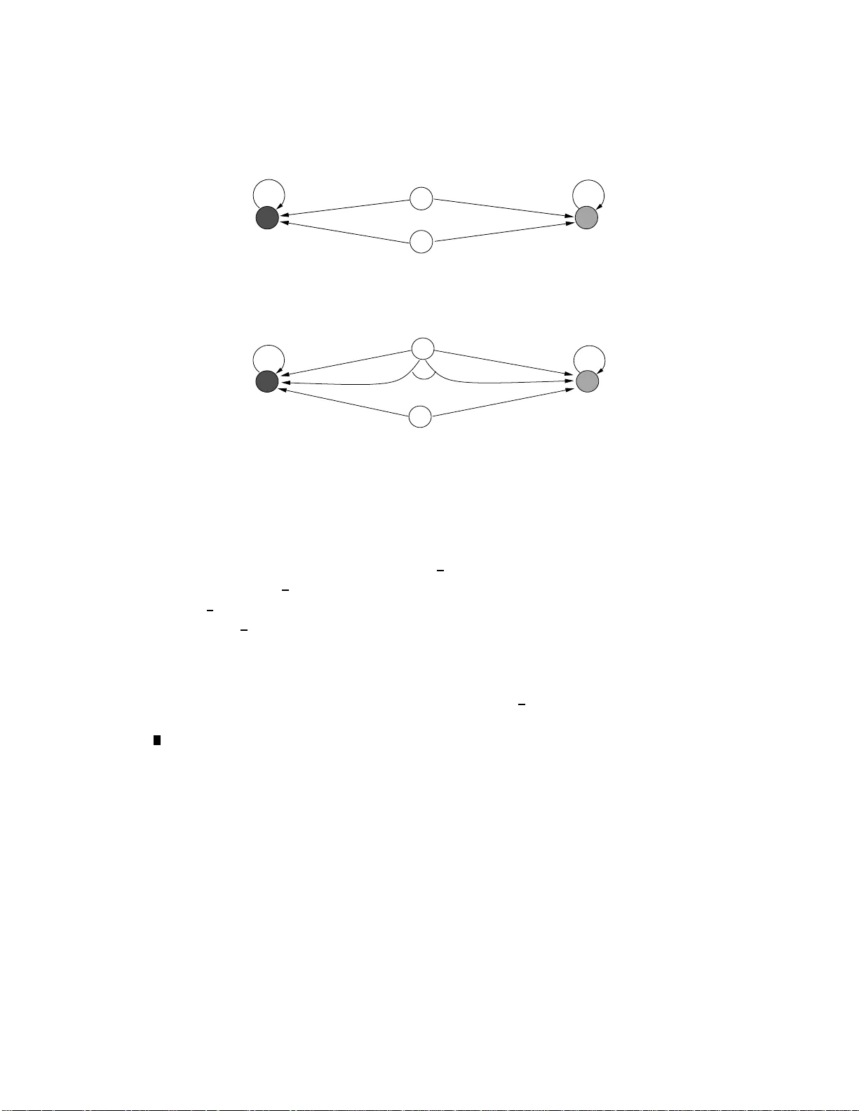
Logical Methods in Computer Science V ol. 4 (3:7) 2008, pp. 1–28 www .lmcs-online.org Submitted Jan. 4, 2008 Published Sep . 11, 2008 GAME REFINEMENT RELA TIONS AND METRIC S LUCA DE ALF ARO a , RUP AK MAJUMDAR b , VISHW ANA TH RAMAN c , AND MARI ¨ ELLE STOELINGA d a CE Department, Unive rsit y of Calif ornia, Santa Cruz e-mail addr ess : luca@soe.ucsc.edu b Department of C S, Universit y of Califo rnia, Los Angeles e-mail addr ess : rupak@cs.ucla.edu c CS Department, Univ ersit y of Cali fornia, S anta Cruz e-mail addr ess : vishw a@so e.ucsc.edu d Department of CS, Universit y of Tw en te, The Netherlands e-mail addr ess : marielle@cs.ut wen te.nl Abstra ct. W e consider tw o-play er games play ed over ﬁnite state spaces for an inﬁnite num ber of roun ds. At each state, the play ers simultaneo usly choose mo ves; the mov es determine a successor state. It is often adva ntag eous for p la ye rs to choose probabilit y dis- tributions o ver mo ves, rather than single mo ves. Given a goal (e.g., “reach a target state”), the qu estion of winning is thus a probabilistic one: “what is the maximal p robabilit y of winning from a give n state?”. On these game structures, t w o fund amen tal notions are those of e quivalenc es and met- rics . Give n a set of winning conditions, tw o states are e qui valent if th e play ers can win the same games with th e same probability from b oth states. M etrics provide a b ound on the d iﬀerence in the probabilities of winning across states, capturing a qu antita tive n otion of state “similarit y”. W e introduce equiv alences and metrics for tw o-pla yer game stru ctures, and we show that they characterize t he diﬀerence in probabilit y of winning games whose goals are expressed in th e qu an titative µ - calculus. The qu antita tive µ -calculus can exp ress a large set of goals, including reachabilit y , safet y , and ω -regular prop erties. Thus, we claim th at our relations and metrics provide th e canonical ex tensions to games, of the classical n otion of bisimulation for transition sy stems. W e develop our results b oth for equiv alences and metrics, whic h generalize bisim ulation, and for asymmetrical versi ons, which generalize sim ulation. 1998 ACM Subje ct Classiﬁc ation: F.4.1, F.1.1. Key wor ds and phr ases: game semantics, minimax t h eorem, metrics, ω -regular prop erties, quantitativ e µ -calculus, probabilistic choice, eq uiv alence of states, reﬁn ement of states. ∗ A versio n of this pap er t itled “Game Relations and Metrics” app eared in th e 22 nd Annual IEEE Sym- p osium on Logic in Computer Science, July 2007. LOGICAL METHODS l IN COMPUTER SCIENCE DOI:10.216 8/LMCS-4 (3:7) 2008 c  L. de Alfaro, R. Majumdar, V . Raman, and M. Stoelinga CC  Cre ative Commons 2 L. DE ALF A RO, R. MA JUM DAR, V. RAMA N, A ND M. STOELINGA 1. Introduction W e consider t w o-pla y er games p la yed for an inﬁ nite num b er of round s o ver ﬁnite state spaces. A t eac h round , the pla y ers simultaneously and ind ep endentl y select mov es; the mo v es then d etermine a probabilit y d istribution o v er su ccessor states. These games, kn own v ariously as sto chastic games [27 ] or c oncurr ent games [5, 1, 7 ], generalize m an y common structures in computer science, from transition systems, to Marko v chains [15] and Mark o v decision pr o cesses [8]. The games are turn-b ase d if, at eac h state, at most one of the play ers has a c h oice of mo v es, and deterministic if the su ccessor state is uniquely determined by the current state, and b y the mo v es c hosen by the play ers. It is well-kno wn that in such games w ith simultaneous mov es it is often adv an tageous for the pla y ers to randomize their mo v es, so that at eac h r ound, th ey pla y n ot a single “pu re” mo v e, bu t rather, a probabilit y distribution o ver the a v ailable mo v es. These probabilit y distributions o v er mov es, called mixe d moves [23], lead to v arious notions of equilibria [32, 23], such as the equilibriu m result expressed by the minimax theorem [32]. Intuiti v ely , the b eneﬁ t of p la ying mixed, rather than p ure, mo v es lies in p rev en ting the adve rsary from tailoring a resp onse to the ind ivid ual mo ve pla y ed. Eve n for simple reac habilit y games, the use of mixed mo v es ma y allo w pla yers to w in , w ith probabilit y 1, games that they would lose (i.e., w in w ith p robabilit y 0) if restricted to playi ng pur e mov es [5]. With mixed m o ves, the question of winning a game w ith resp ect to a goal is thus a pr obabilistic one: what is the maximal probability a p lay er can b e guarantee d of w in ning, r egardless of h o w the other pla y er pla ys ? This p robabilit y is kno wn, in brief, as the winning pr ob ability. In structures ranging from transition systems to Mark o v d ecision pr o cesses and games, a fun d amen tal question is th e one of e quivalenc e of states. Given a su itably large class Φ of p rop erties, contai ning all pr op erties of inte rest to th e mo deler, t w o s tates are equiv alent if the same prop erties hold in b oth states. F or a p r op ert y ϕ , d enote the v alue of ϕ at s by ϕ ( s ): in the case of games, this might repr esen t the maximal probabilit y of a pla yer w inning with resp ect to a goal expr essed b y ϕ . Tw o states s and t are equiv alent if ϕ ( s ) = ϕ ( t ) for all ϕ ∈ Φ. F or (ﬁ nite-branc hing) trans ition sys tems, and for the class of prop erties Φ expressible in the µ -calculus [17], state equiv alence is captured b y bisim ulation [22]; for Mark o v decision pr o cesses, it is captured by pr obabilistic bisim ulation [25]. F or quantita tiv e prop erties, a notion r elated to equiv alence is that of a metric: a metric provides a tigh t b ound for how m uc h the v alue of a pr op ert y can d iﬀer at states of the system, and provi des th us a quan titativ e notion of similarit y b et w een states. Give n a set Φ of p rop erties, the metric distance of tw o states s and t can b e deﬁned as sup ϕ ∈ Φ | ϕ ( s ) − ϕ ( t ) | . Metrics for Mark o v decision pro cesses h a ve b een studied in [9, 30, 31, 10 , 11]. Obviously , the metrics and relations are connected, in the sense that the relations are the kernels of th e metrics (the pairs of states h a v in g metric distance 0). The metrics and relations are at th e h eart of many v eriﬁcation tec h niques, from app ro ximate reasoning (one can su bstitute states that are close in the metric) to system reductions (one can collapse equiv alent states) to comp ositional reasoning and reﬁn ement (providing a notion of su bstitutivit y of equ iv alen ts). W e introd u ce metrics and equiv alence r elatio ns for concurrent games, with r esp ect to the class of prop erties Φ expr essib le in the quan tita tiv e µ -calculus [7 , 21]. W e claim th at these metrics and relations r epresen t the canonical extension of bisimulat ion to games. W e also in tr o duce asymmetrical ve rsions of these metrics and equiv alence s, whic h constitute the canonical extension of simulati on. GAME REFINEMENT RELA TIONS AND METRICS 3 An equiv alence relation for deterministic games that are either turn -based, or wh ere the p la yers are constrained to pla ying pu re mov es, has b een introd uced in [2] and called alternating bisimulation. Relations an d metrics for the general case of concurren t games ha v e so far prov ed elus iv e, with some previous attempts at their deﬁnition by a sub set of the authors f ollo wing a su btly ﬂa w ed approac h [6, 19]. The cause of the diﬃculty go es to the heart of the deﬁnition of bisim ulation. In the deﬁnition of b isimulation f or transition systems, for ev ery pair s , t of b isimilar states, w e r equire that if s can go to a state s ′ , then t should b e able to go to t ′ , such that s ′ and t ′ are again bisimilar (w e also ask that s , t hav e an equiv alen t p redicate v aluation). Th is deﬁnition has b een extended to Mark ov decision pro cesses by requiring that for ev ery mixed mo v e from s , there is a mixed mo v e from t , su c h that the m ov es indu ce prob ab ility distributions o ver successor states that are equiv alen t mod ulo the underlyin g bisim ulation [25, 24]. Unfortunately , the generaliza tion of this app ealing deﬁnition to games f ails. It tu rns out, as we pr o ve in this p ap er, that requiring pla y ers to b e able to replicate pr obabilit y distribu tions ov er successors (mo dulo the u nderlying equiv alence) leads to an equiv alence that is too ﬁne, and that m ay fail to relate states at wh ic h the same quan titati v e µ -calculus form u las hold. W e sh o w that phrasing the d eﬁnition in terms of distributions o v er su ccessor states is the wr on g ap p roac h for games; rather, the d eﬁnition should b e ph r ased in terms of exp ectatio ns of certain metric-b ounded quanti ties. Our starting p oin t is a closer lo ok at the deﬁnition of metrics for Mark ov decision pro cesses. W e observ e that we can manipulate the deﬁnition of metrics giv en in [31], obtaining an alternativ e form, whic h we call the a priori form, in con trast w ith the original form of [31], whic h we call th e a p osteriori form. Informally , the a p osteriori form is the traditional deﬁnition, phr ased in terms of s im ilarity of p robabilit y distr ibutions; th e a priori form is instead p hrased in terms of exp ectations. W e s ho w that, while on Mark o v decision pro cesses these t w o forms coincide, this is not the case for games; moreov er, we sho w that it is the a priori form that provides the canonical metrics for games. W e p ro v e that the a priori m etric d istance b etw een t w o states s an d t of a concurrent game is equal to su p ϕ ∈ Φ | ϕ ( s ) − ϕ ( t ) | , wh ere Φ is the set of pr op erties expressib le via the quan titativ e µ -calculus. This r esu lt can b e su mmarized by sa ying that the quan titat iv e µ -calculus pr o vides a lo gic al char acterization for the a priori m etrics, similar to the wa y the ordinary µ -calculus pro vides a logic al c haracteriza tion of b isim ulation. F u rthermore, we pro v e that a pr iori metrics — and their k ernels, the a priori relations — satisfy a r e ci pr o city prop erty , stating that pr op erties expr essed in term s of play er 1 and p lay er 2 w inning con- ditions ha ve the same distin gu ish ing p o wer. T his pr op ert y is in timately connected to the fact that concurrent games, pla y ed with mixed m o ves, are determine d for ω -regular goals [20, 7]: the probability that pla y er 1 ac h iev es a goal ψ is one min us the probabilit y that pla y er 2 ac h iev es the goal ¬ ψ . Recipro cit y ensu res that there is one, canonical, notion of game equiv alence. This is in contrast to the case of alternating bisim ulation of [2], in which there are distinct p la yer 1 and play er 2 v ersions, as a consequence of the f act that concurrent games, when play ed with pure mov es, are not determined. The logical charac terizatio n and recipro cit y r esult justify our claim that a priori metrics and r elations are the canonical no- tion of metrics, and equiv alence, for concurrent games. Neither the logical charact erization nor the r ecipro cit y result hold for the a p osteriori m etrics and relations. While this intro d uction fo cused mostly on metrics and equ iv alence relations, w e also dev elop r esults f or the asym m etrical v ersions of these notions, related to simulatio n. 4 L. DE ALF A RO, R. MA JUM DAR, V. RAMA N, A ND M. STOELINGA 2. Games and Goals W e will d ev elop metrics f or game stru ctures o ver a set S of s tates. W e s tart with some preliminary deﬁn itions. F or a ﬁnite set A , let Dist( A ) = { p : A 7→ [0 , 1] | P a ∈ A p ( a ) = 1 } denote the s et of probabilit y d istributions o ver A . W e say that p ∈ Dist( A ) is deterministic if th ere is a ∈ A suc h th at p ( a ) = 1. F or a set S , a valuation over S is a function f : S 7→ [0 , 1] asso ciating with ev ery elemen t s ∈ S a v alue 0 ≤ f ( s ) ≤ 1; we let F b e the set of all v aluations. F or c ∈ [0 , 1], we denote by c th e constan t v aluation suc h that c ( s ) = c at all s ∈ S . W e order v aluations p oint wise: for f , g ∈ F , w e write f ≤ g iﬀ f ( s ) ≤ g ( s ) at all s ∈ S ; we remark that F , under ≤ , forms a complete lattice. Giv en a, b ∈ I R, we write a ⊔ b = max { a, b } , and a ⊓ b = min { a, b } ; w e also let a ⊕ b = min { 1 , max { 0 , a + b }} and a ⊖ b = max { 0 , min { 1 , a − b }} . W e extend ⊓ , ⊔ , + , − , ⊕ , ⊖ to v aluations by inte rpreting them in p oin t wise f ash ion. A dir e cte d metric is a fu nction d : S 2 7→ I R ≥ 0 whic h satisﬁes d ( s, s ) = 0 and d ( s, t ) ≤ d ( s, u ) + d ( u, t ) f or all s, t, u ∈ S . W e denote by M ⊆ S 2 7→ I R the space of all metrics; this space, order ed p oint wise, forms a latt ice whic h w e indicate with ( M , ≤ ). Give n a metric d ∈ M , w e d enote by ˘ d its opp osite version, deﬁned by ˘ d ( s, t ) = d ( t, s ) for all s, t ∈ S ; we sa y that d is symmetrical if d = ˘ d . 2.1. Game Structures. W e assume a ﬁxed, ﬁnite set V of observation variables . A (t wo- pla y er, concurr en t) game structur e G = h S, [ · ] , Moves , Γ 1 , Γ 2 , δ i consists of the follo wing comp onen ts [1, 5]: • A ﬁn ite set S of states. • A v ariable in terpretation [ · ] : V × S 7→ [0 , 1], which asso ciates with eac h v ariable v ∈ V a v aluation [ v ]. • A ﬁn ite set Moves of mo ves. • Tw o mov e assignmen ts Γ 1 , Γ 2 : S 7→ 2 Moves \ ∅ . F or i ∈ { 1 , 2 } , the assignment Γ i asso ciates with eac h state s ∈ S the nonempty set Γ i ( s ) ⊆ Moves of mo v es a v ailable to pla y er i at state s . • A probabilistic transition fun ction δ : S × Moves × Moves 7→ Dist( S ), that giv es the probabilit y δ ( s, a 1 , a 2 )( t ) of a transition f r om s to t when play er 1 p la ys mo v e a 1 and pla y er 2 pla ys mo v e a 2 . A t ev ery state s ∈ S , play er 1 c ho oses a mo v e a 1 ∈ Γ 1 ( s ), and sim ultaneously and inde- p endently p la yer 2 c h o oses a mo v e a 2 ∈ Γ 2 ( s ). The game then pro ceeds to the su cces- sor state t ∈ S with p robabilit y δ ( s , a 1 , a 2 )( t ). W e d enote by Dest( s, a 1 , a 2 ) = { t ∈ S | δ ( s, a 1 , a 2 )( t ) > 0 } the set of destination states when actions a 1 , a 2 are c h osen at s . The v ariables in V naturally induce an equ iv alence on states: f or states s , t , deﬁne s ≡ t if for all v ∈ V w e ha v e [ v ]( s ) = [ v ]( t ). In the follo w ing, un less otherwise noted, th e deﬁn itions r efer to a game structure with comp onents G = h S, [ · ] , Moves , Γ 1 , Γ 2 , δ i . F or pla y er i ∈ { 1 , 2 } , w e wr ite ∼ i = 3 − i for the opp onent. W e also consider the f ollo wing sub classes of game structures. • T urn-b ase d game structur es. A game structure G is turn-b ase d if we can write S as the disjoin t un ion of tw o sets: the set S 1 of player 1 states, and the set S 2 of player 2 states, suc h that s ∈ S 1 implies | Γ 2 ( s ) | = 1, and s ∈ S 2 implies | Γ 1 ( s ) | = 1, and fur ther, there GAME REFINEMENT RELA TIONS AND METRICS 5 is a sp ecial v ariable turn ∈ V , su c h that [ turn ]( s ) = 1 iﬀ s ∈ S 1 , and [ turn ]( s ) = 0 iﬀ s ∈ S 2 : th u s , the v ariable turn indicates whose tur n it is to play at a state. • Markov de c i sion pr o c esses. A game structur e G is a Markov de cision pr o c ess (MDP) [8] if only one of th e t w o pla yers has a choic e of m o ves. F or i ∈ { 1 , 2 } , we sa y that a structure is an i -MDP if ∀ s ∈ S , | Γ ∼ i ( s ) | = 1. F or MDPs, w e omit the (single) mov e of the p la yer without a c hoice of mo v es, and write δ ( s, a ) for the transition function. • Deterministic game structur es. A game structure G is deterministic if, for all s ∈ S , a 1 ∈ M oves , and a 2 ∈ Moves , there exists a t ∈ S suc h that δ ( s, a 1 , a 2 )( t ) = 1; we denote su c h t b y τ ( s, a 1 , a 2 ). W e sometimes call pr ob abilistic a general game structur e, to emphasize the fact that it is not necessarily d eterministic. Note th at MDPs can b e seen as turn-based games by setting [ turn ] = 1 for 1-MDPs and [ turn ] = 0 for 2-MDPs. Pure and mixed mov es. A mixe d move is a probabilit y distribution ov er the mov es a v aila ble to a pla y er at a state. W e denote by D i ( s ) = Dist(Γ i ( s )) the set of mixed mo v es a v aila ble to p la yer i ∈ { 1 , 2 } at s ∈ S . The mo v es in Moves are called pur e moves, in con tr ast to mixed mov es. W e extend the transition fu nction to mixed mo ves. F or s ∈ S and x 1 ∈ D 1 ( s ), x 2 ∈ D 2 ( s ), we write δ ( s, x 1 , x 2 ) for the next-state p robabilit y d istribution induced b y the mixed mo v es x 1 and x 2 , deﬁned for all t ∈ S b y δ ( s, x 1 , x 2 )( t ) = X a 1 ∈ Γ 1 ( s ) X a 2 ∈ Γ 2 ( s ) δ ( s, a 1 , a 2 )( t ) x 1 ( a 1 ) x 2 ( a 2 ) . In the follo wing, we sometimes restrict th e mov es of the p lay ers to pu r e mo v es. W e iden tify a pur e mo v e a ∈ Γ i ( s ) a v ailable to pla y er i ∈ { 1 , 2 } at a state s with a deterministic distribution that plays a with pr obabilit y 1. The deterministic setting. The deterministic setting is obtained b y considering d eter- ministic game structures, with play ers restricted to pla ying pure mo v es. 2.2. Predecessor op erators. Given a v aluatio n f ∈ F , a state s ∈ S , and t w o mixed mo v es x 1 ∈ D 1 ( s ) and x 2 ∈ D 2 ( s ), w e deﬁne the exp ectation of f from s under x 1 , x 2 : E x 1 ,x 2 s ( f ) = X t ∈ S δ ( s, x 1 , x 2 )( t ) f ( t ) . F or a game str ucture G , for i ∈ { 1 , 2 } w e d eﬁ ne the valuation tr ansformer Pre i : F 7→ F b y , for all f ∈ F and s ∈ S , Pre i ( f )( s ) = sup x i ∈D i ( s ) inf x ∼ i ∈D ∼ i ( s ) E x 1 ,x 2 s ( f ) . In tuitiv ely , Pre i ( f )( s ) is the maximal exp ectati on pla yer i can ac h iev e of f after one step from s : this is the classica l “one-da y” or “next-stage” op erator of the theory of r ep eated games [12]. W e also deﬁn e a deterministic v ersion of this op erator, in whic h pla y ers are forced to pla y pure mo v es: Pre Γ i ( f )( s ) = max x i ∈ Γ i ( s ) min x ∼ i ∈ Γ ∼ i ( s ) E x 1 ,x 2 s ( f ) . 6 L. DE ALF A RO, R. MA JUM DAR, V. RAMA N, A ND M. STOELINGA 2.3. Quantitativ e µ - calculus. W e consider the set of prop erties expressed by the quanti- tative µ -c alculus ( q µ ). As d iscussed in [16, 7, 21], a large set of pr op erties can b e enco ded in q µ , sp anning from basic pr op erties such as maximal reac habilit y and safety probability , to the maximal probability of satisfying a general ω -regular sp eciﬁcation. Syn tax. Th e syntax of q u an titati v e µ -calculus is deﬁned with resp ect to the set of obser- v ation v ariables V as w ell as a set MV ars of c alculus variables, w h ic h are distinct fr om the observ ation v ariables in V . The synta x is giv en as follo w s: ϕ ::= c | v | Z | ¬ ϕ | ϕ ∨ ϕ | ϕ ∧ ϕ | ϕ ⊕ c | ϕ ⊖ c | pre 1 ( ϕ ) | pre 2 ( ϕ ) | µZ. ϕ | ν Z. ϕ for constan ts c ∈ [0 , 1], observ ation v ariables v ∈ V , and calculus v ariables Z ∈ MV ars . In the form ulas µZ. ϕ and ν Z. ϕ , we fur thermore require that all o ccurr ences of the b oun d v ariable Z in ϕ o ccur in the scop e of an ev en num b er of occur rences of the complemen t op erator ¬ . A f orm ula ϕ is close d if ev ery calculus v ariable Z in ϕ o ccurs in the scope of a qu an tiﬁer µZ or ν Z . F rom no w on, with abuse of n otatio n, w e d enote by q µ the set of closed form ulas of q µ . A formula is a player i f ormula, for i ∈ { 1 , 2 } , if ϕ do es n ot contai n the pre ∼ i op erator; we den ote with q µ i the synta ctic su bset of q µ consisting on ly of closed pla y er i formulas. A f orm ula is in p ositive form if the negation app ears only in front of observ ation v ariables, i.e., in the conte xt ¬ v ; we denote w ith q µ + and q µ + i the sub sets of q µ and q µ i consisting only of p ositiv e formula s. W e remark that the ﬁxp oin t op erators µ an d ν will not b e n eeded to ac hieve our results on the logica l characte rization of game relatio ns. T hey ha v e b een included in the calculus b ecause they allo w the exp r ession of man y in teresting prop erties, suc h as safet y , reac h ab ility , and in general, ω -regular prop erties. The op erators ⊕ and ⊖ , on the other hand, are necessary for our results. Seman tics. A v ariable v aluation ξ : MV ars 7→ F is a fu nction that maps eve ry v ariable Z ∈ MV ars to a v aluation in F . W e write ξ [ Z 7→ f ] for the v aluation that agrees with ξ on all v ariables, except th at Z is mapp ed to f . Give n a game stru cture G and a v ariable v aluation ξ , ev ery form ula ϕ of the quan titativ e µ -calculus deﬁnes a v aluation [ [ ϕ ] ] G ξ ∈ F (the sup erscript G is omitted if th e game structur e is clear fr om the con text): [ [ c ] ] ξ = c [ [ v ] ] ξ = [ v ] [ [ Z ] ] ξ = ξ ( Z ) [ [ ¬ ϕ ] ] ξ = 1 − [ [ ϕ ] ] ξ [ [ ϕ  ⊕ ⊖  c ] ] ξ = [ [ ϕ ] ] ξ  ⊕ ⊖  c [ [ ϕ 1  ∨ ∧  ϕ 2 ] ] ξ = [ [ ϕ 1 ] ] ξ  ⊔ ⊓  [ [ ϕ 2 ] ] ξ [ [pr e i ( ϕ )] ] ξ = Pre i ([ [ ϕ ] ] ξ ) [ [  µ ν  Z. ϕ ] ] ξ =  inf sup  { f ∈ F | f = [ [ ϕ ] ] ξ [ Z 7→ f ] } where i ∈ { 1 , 2 } . The existence of the ﬁxp oin ts is guaran teed by the monotonicit y and con tinuit y of all op erators and can b e computed by Picard iteratio n [7]. If ϕ is closed, [ [ ϕ ] ] ξ is in dep endent of ξ , and we wr ite simp ly [ [ ϕ ] ]. W e also d eﬁne a deterministic seman tics [ [ · ] ] Γ for q µ , in whic h pla yers can select only pure m o ves in the op erators pr e 1 , pre 2 . [ [ · ] ] Γ is d eﬁned as [ [ · ] ], except for the clause [ [pr e i ( ϕ )] ] Γ ξ = Pre Γ i ([ [ ϕ ] ] Γ ξ ) . GAME REFINEMENT RELA TIONS AND METRICS 7 Example 1. Giv en a set T ⊆ S , the char acteristic valuation T of T is deﬁn ed by T ( s ) = 1 if s ∈ T , and T ( s ) = 0 otherw ise. With this n otation, the maximal p robabilit y with wh ic h pla y er i ∈ { 1 , 2 } can ensu re even tually reac hin g T ⊆ S is giv en b y [ [ µZ . ( T ∨ pre i ( Z ))] ], and the maximal probability w ith which pla yer i can guarantee sta yin g in T foreve r is giv en by [ [ ν Z. ( T ∧ pre i ( Z ))] ] (see, e.g., [7]). The ﬁrst p rop ert y is called a r e achability prop er ty , the second a safety prop erty . 3. Metrics W e are interested in devel oping a metric on s tates of a game structure that captures an appro ximate n otion of equiv alence: states close in the metric should yield s imilar v alues to the pla y ers for any w inning ob jectiv e. S p eciﬁcally , we are in terested in deﬁ n ing a b isim ula- tion metric [ ≃ g ] ∈ M su c h that for any game s tr ucture G and states s, t of G , the follo wing con tinuit y prop ert y h olds: [ ≃ g ]( s, t ) = sup ϕ ∈ q µ | [ [ ϕ ] ]( s ) − [ [ ϕ ] ]( t ) | . (3.1) In p articular, the kernel of th e metric, that is, states at distance 0, are equiv alent: eac h pla y er can get exactly the same v alue from either state for any ob j ective . Notice that in deﬁning th e metric indep endent of a pla y er, we are exp ecting our metrics to b e r e c ipr o c al , that is, in v arian t under a c hange of p la yer. Reciprocity is exp ected to hold since the underlying games w e consider are determined —for an y game, the v alue obtained b y pla yer 2 is one minus the v alue obtained by play er 1— and yields canonical m etrics on games. Th us, our metrics will generalize equ iv alence and r eﬁnemen t relations that hav e b een studied on MDPs and in the deterministic setting. T o un derline the connection b et w een classical equiv alences and the metrics we deve lop, w e write [ s ≃ g t ] for [ ≃ g ]( s, t ), so that the desired prop erty of the bisimulatio n metric can b e stated as [ s ≃ g t ] = sup ϕ ∈ q µ | [ [ ϕ ] ]( s ) − [ [ ϕ ] ]( t ) | . Metrics of this t yp e hav e already b een dev eloped f or Mark o v decision pro cesses (MDPs) [30, 10]. Our construction of metrics for games starts fr om an analysis of these constru ctions. 3.1. Metrics for MDPs. W e consider the case of 1-MDPs; the case for 2-MDPs is sym- metrical. Th roughout this subsection, w e ﬁx a 1-MDP h S, [ · ] , Moves , Γ 1 , Γ 2 , δ i . Before we present the metric corresp ondent of probabilistic sim ulation, w e ﬁr st reph rase classical p rob- abilistic (bi)sim ulation on MDPs [18, 14, 25, 26] as a ﬁxp oin t of a r elation tr ansformer. As a ﬁ rst step, w e lift relations b et ween states to relatio ns b etw een distributions. Giv en a relation R ⊆ S × S and t w o distrib utions p, q ∈ Dist( S ), we let p ⊑ R q if there is a function ∆ : S × S → [0 , 1] such that: • ∆( s, s ′ ) > 0 imp lies ( s, s ′ ) ∈ R ; • p ( s ) = P s ′ ∈ S ∆( s, s ′ ) for an y s ∈ S ; • q ( s ′ ) = P s ∈ S ∆( s, s ′ ) for an y s ′ ∈ S . T o reph rase probabilistic simulati on, we deﬁne the relation transformer F : 2 S × S 7→ 2 S × S as follo w s . F or all relations R ⊆ S × S and s, t ∈ S , w e let ( s, t ) ∈ F ( R ) iﬀ s ≡ t ∧ ∀ x 1 ∈D 1 ( s ) . ∃ y 1 ∈D 1 ( t ) . δ ( s, x 1 ) ⊑ R δ ( t, y 1 ) , (3.2) 8 L. DE ALF A RO, R. MA JUM DAR, V. RAMA N, A ND M. STOELINGA for all states s, t ∈ S . Probabilistic simulat ion is the greatest ﬁxp oin t of (3.2); pr ob ab ilistic bisim ulation is the greatest symmetrical ﬁ xp oint of (3.2). T o obtain a metric equiv alen t of probabilistic sim ulation, w e lift the ab o ve ﬁ xp oint from relations (subsets of S 2 ) to metrics (maps S 2 7→ I R ). First, we deﬁne [ ≡ ] ∈ M for all s, t ∈ S by [ s ≡ t ] = max v ∈V | [ v ]( s ) − [ v ]( t ) | . Second, we lift (3.2 ) to metrics, deﬁn ing a metric transformer H 1MDP p ost : M 7→ M . F or all d ∈ M , let D ( δ ( s, x 1 ) , δ ( t, y 1 ))( d ) b e the distribution distanc e b etw een δ ( s, x 1 ) and δ ( t, y 1 ) with r esp ect to the metric d . W e will sho w later ho w to d eﬁ ne su c h a distribution distance. F or s, t ∈ S , we let H 1MDP p ost ( d )( s, t ) = [ s ≡ t ] ⊔ su p x 1 ∈D 1 ( s ) inf y 1 ∈D 1 ( t ) D ( δ ( s, x 1 ) , δ ( t, y 1 ))( d ) . (3.3) In this d eﬁ nition, th e ∀ and ∃ of (3.2) ha ve b een replaced by sup and inf , resp ectiv ely . Since equiv alen t states should ha v e d istance 0, th e simulatio n metric in MDPs is deﬁned as the le ast (rather than greatest) ﬁxp oin t of (3.3) [30, 10]. Similarly , the bisim ulation metric is d eﬁned as the least symmetrical ﬁ x p oin t of (3.3). F or a distance d ∈ M an d t wo distribu tions p, q ∈ Dist( S ), th e distribution distanc e D ( p, q )( d ) is a m easure of ho w muc h “w ork” we ha v e to do to mak e p lo ok lik e q , giv en that mo ving a u nit of probabilit y mass f rom s ∈ S to t ∈ S h as cost d ( s, t ). More pr ecisely , D ( p, q )( d ) is deﬁned via the tr ans-shipping pr oblem, as the minimum cost of shipp in g the distribution p into q , with edge costs d . Thus, D ( p, q )( d ) is th e solution of the follo wing linear programming (LP) pr oblem o v er the set of v ariables { λ s,t } s,t ∈ S : Minimize X s,t ∈ S d ( s, t ) λ s,t sub ject to X t ∈ S λ s,t = p ( s ) , X s ∈ S λ s,t = q ( t ) , λ s,t ≥ 0 . Equiv alen tly , w e can deﬁne D ( p, q )( d ) via the du al of the ab o v e LP problem [30]. Give n a metric d ∈ M , let C ( d ) ⊆ F b e the su bset of v aluatio ns k ∈ F s uc h that k ( s ) − k ( t ) ≤ d ( s, t ) for all s , t ∈ S . Then th e dual formula tion is: Maximize X s ∈ S p ( s ) k ( s ) − X s ∈ S q ( s ) k ( s ) (3.4) sub ject to k ∈ C ( d ) . The constrain t C ( d ) on the v aluation k , states that the v alue of k across states cannot diﬀer b y more than d . This means, intuiti v ely , that k b eha v es lik e the v aluation of a q µ form ula: as we will s ee, th e logical c haracteriza tion implies that d is a b oun d for the diﬀerence in v aluation of q µ form ulas across states. In deed, the logical c haracterizatio n of the metrics is pro v ed b y constructing formulas wh ose v aluation appro ximate that of the optimal k . Plugging (3.4) in to (3.3), we obtain: H 1MDP p ost ( d )( s, t ) = [ s ≡ t ] ⊔ sup x 1 ∈D 1 ( s ) inf y 1 ∈D 1 ( t ) sup k ∈ C ( d )  E x 1 s ( k ) − E y 1 t ( k )  . (3.5) W e can in terp ret this deﬁnition as follo ws. State t is tryin g to sim u late state s (this is a deﬁnition of a sim ulation metric). First, state s c h o oses a mixed mo v e x 1 , attempting to mak e sim ulation as hard as p ossible; then, state t chooses a mixed mo ve y 1 , trying to matc h the eﬀect of x 1 . Once x 1 and y 1 ha v e b een c h osen, th e resulting distance b et w een s and t is equal to the maximal diﬀerence in exp ectatio n, for mo ve s x 1 and y 1 , of a v aluation GAME REFINEMENT RELA TIONS AND METRICS 9 k ∈ C ( d ). W e call the metric tr ansformer H 1MDP p ost the a p osteriori metric transf ormer: the v aluation k in (3.5) is c h osen after the mov es x 1 and y 1 are c hosen. W e can deﬁ n e an a priori metric transf ormer, w here k is c h osen b efore x 1 and y 1 : H 1MDP prio ( d )( s, t ) = [ s ≡ t ] ⊔ sup k ∈ C ( d ) sup x 1 ∈D 1 ( s ) inf y 1 ∈D 1 ( t )  E x 1 s ( k ) − E y 1 t ( k )  . (3.6) In tuitiv ely , in the a priori transformer, ﬁrst a v aluation k ∈ C ( d ) is c hosen. Th en, state t m u st sim ulate s tate s with resp ect to the exp ectatio n of k . S tate s chooses a mo v e x 1 , trying to maximize the diﬀerence in exp ectations, and state t chooses a mo v e y 1 , trying to minimize it. The distance b etw een s and t is then equal to the diﬀerence in the resu lting exp ectations of k . Theorem 3.1 b elo w states that f or MDPs, a priori and a p osteriori sim ulation metrics coincide. In the next section, we will see th at th is is not the case for games. Theorem 3.1. F or al l MDPs, H 1MDP p ost = H 1MDP prio . Pr o of. Consid er t w o states s, t ∈ S , and a metric d ∈ M . W e ha v e to p ro v e that sup k sup x 1 inf y 1 [ E x 1 s ( k ) − E y 1 t ( k )] = sup x 1 inf y 1 sup k [ E x 1 s ( k ) − E y 1 t ( k )] . (3.7) In the left-hand side, we can exc hange th e tw o outer sups. Th en, noticing th at the diﬀerence in exp ectation is bi-linear in k and y 1 for a ﬁxed x 1 , that y 1 is a probabilit y distribution, and that k is chosen fr om a compact con v ex subset, we app ly th e generalized minimax theorem [28] to exc h ange sup k inf y 1 in to inf y 1 sup k , th us obtaining the right -hand side. The metrics d eﬁned ab o ve are logically characte rized b y q µ . Precisely , let [ ∼ ] ∈ M b e the least symmetrical ﬁxp oin t of H 1MDP prio = H 1MDP p ost . Then , L emma 5 . 24 and Corollary 5 . 25 of [10], (originally stated for H 1MDP p ost ) state that for all states s , t of a 1-MDP , we hav e [ s ∼ t ] = sup ϕ ∈ q µ | [ [ ϕ ] ]( s ) − [ [ ϕ ] ]( t ) | . 3.2. Metrics for C oncurrent Games. W e no w extend the sim ulation and bisimulat ion metrics from MDPs to general game structures. As we s h all see, unlike for MDPs, the a priori and th e a p osteriori metrics do not coincide ov er games. In particular, we sh o w that the a priori form ulation satisﬁes b oth a tigh t logical c haracterizatio n as well as recipro cit y while, p erh aps surpr isingly , the more n atural a p osteriori v ersion do es not. A p osteriori metrics are deﬁ n ed via the metric trans f ormer H ⊑ 1 : M 7→ M as follo w s, for all d ∈ M and s , t ∈ S : H ⊑ 1 ( d )( s, t ) = [ s ≡ t ] ⊔ sup x 1 ∈D 1 ( s ) inf y 1 ∈D 1 ( t ) sup y 2 ∈D 2 ( t ) inf x 2 ∈D 2 ( s ) D ( δ ( s, x 1 , x 2 ) , δ ( t, y 1 , y 2 ) , d ) = [ s ≡ t ] ⊔ sup x 1 ∈D 1 ( s ) inf y 1 ∈D 1 ( t ) sup y 2 ∈D 2 ( t ) inf x 2 ∈D 2 ( s ) sup k ∈ C ( d )  E x 1 ,x 2 s ( k ) − E y 1 ,y 2 t ( k )  . (3.8) 10 L. DE ALF A RO, R. MA JUM DAR, V. RAMA N, A ND M. STOELINGA A priori metrics are d eﬁned b y bringing the su p k outside. Precisely , we deﬁn e a metric transformer H  1 : M 7→ M as follo ws, f or all d ∈ M and s , t ∈ S : H  1 ( d )( s, t ) = [ s ≡ t ] ⊔ s u p k ∈ C ( d ) sup x 1 ∈D 1 ( s ) inf y 1 ∈D 1 ( t ) sup y 2 ∈D 2 ( t ) inf x 2 ∈D 2 ( s )  E x 1 ,x 2 s ( k ) − E y 1 ,y 2 t ( k )  = [ s ≡ t ] ⊔ sup k ∈ C ( d ) h sup x 1 ∈D 1 ( s ) inf x 2 ∈D 2 ( s ) E x 1 ,x 2 s ( k ) − sup y 1 ∈D 1 ( t ) inf y 2 ∈D 2 ( t ) E y 1 ,y 2 t ( k ) i = [ s ≡ t ] ⊔ sup k ∈ C ( d )  Pre 1 ( k )( s ) − Pre 1 ( k )( t )  . (3.9) First, w e sho w th at H  1 and H ⊑ 1 are monotonic in the lattice of metrics ( M , ≤ ). Lemma 3.2. The fu nc tions H  1 and H ⊑ 1 ar e monotonic in the lattic e of metrics ( M , ≤ ) . Pr o of. F or d, d ′ ∈ M , d ≤ d ′ implies C ( d ) ⊆ C ( d ′ ), and hence sup k ∈ C ( d ) (Pre 1 ( k )( s ) − Pre 1 ( k )( t )) ≤ sup k ∈ C ( d ′ ) (Pre 1 ( k )( s ) − Pre 1 ( k )( t )). This sh o w s th e monotonicit y of H  1 . The monotonicit y of H ⊑ 1 can b e shown in a similar fashion. F rom d ≤ d ′ , reasoning as b efore w e obtain sup k ∈ C ( d )  E x 1 ,x 2 s ( k ) − E y 1 ,y 2 t ( k )  ≤ sup k ∈ C ( d ′ )  E x 1 ,x 2 s ( k ) − E y 1 ,y 2 t ( k )  . The result then f ollo ws fr om the monotonicit y of the op er ators su p x 1 ∈D 1 ( s ) , inf y 1 ∈D 1 ( t ) , sup y 2 ∈D 2 ( t ) , inf x 2 ∈D 2 ( s ) . On the basis of this lemma, we can d eﬁne the least ﬁx p oin ts of H  1 and H ⊑ 1 , w hic h will yield our game simulatio n and bisimulation metrics. Deﬁnition 3.3. A priori metrics: • The a priori simulation metric [  1 ] is the least ﬁxp oint of H  1 . • The a priori bisimulation metric [ ≃ 1 ] is the least symmetrical ﬁxp oint of H  1 . A p osteriori metrics: • The a p osteriori game simulation metric [ ⊑ 1 ] is the least ﬁxp oin t of H ⊑ 1 . • The a p osteriori game bisimulation metric [ ∼ = 1 ] is the least sym metrical ﬁxp oin t of H ⊑ 1 . By exc hanging the roles of the pla yers, w e deﬁne the m etric transformers H  2 and H ⊑ 2 , and the metrics [  2 ], [ ≃ 2 ], [ ⊑ 2 ], [ ∼ = 2 ]. W e n ote that the a p osteriori sim ulation metric [ ⊑ 1 ] has b een introdu ced in [6, 19]. W e also note that the a p osteriori b isim ulation metric [ ∼ = i ] can b e deﬁn ed as the least ﬁxp oin t of H ∼ = i : M 7→ M , deﬁned for all d ∈ M and i ∈ { 1 , 2 } by H ∼ = 1 ( d ) = H ⊑ 1 ( d ) ⊔ Opp ( H ⊑ 1 ( d )) , (3.10) where Opp ( d ) = ˘ d denotes the op p osite of a metric d . Similarly , the a priori bisim ulation metric [ ≃ i ] can b e deﬁn ed as the least ﬁxp oint of H ≃ i : M 7→ M , deﬁned for all d ∈ M and i ∈ { 1 , 2 } by H ≃ 1 ( d ) = H  1 ( d ) ⊔ Opp ( H  1 ( d )) . (3.11) W e wish to s ho w that the metrics of Deﬁnition 3.3 can b e computed via Picard iteration. T o this end , it is n ecessary to sho w th at the op erators H ⊑ 1 and H  1 on the lattice ( M , ≤ ) are up p er semi-con tinuous. I n fact, a very similar pr o of sho ws that th e op erators are lo w er semi-con tinuous, and thus, conti n uous; we omit the pr o of of this more general fact as it is not required for the desired r esult ab out the ap p licabilit y of P icard iteration. GAME REFINEMENT RELA TIONS AND METRICS 11 Lemma 3.4. The op er ators H  1 and H ⊑ 1 on the lattic e ( M , ≤ ) ar e upp er semi-c ontinuous. Pr o of. Let D ⊆ M b e an arb itrary set of distances, and let d ∗ = sup D ; note that d ∗ exists, as ( M , ≤ ) is a complete lattice. W e ﬁrst p ro v e the result for H  1 . W e n eed to prov e that H  1 (sup D ) = s up d ∈ D H  1 ( d ), whic h we abb reviate H  1 (sup D ) = su p H  1 ( D ). In one dir ection, H  1 (sup D ) ≥ s up H  1 ( D ) follo ws from the monotonicit y of H  1 (Lemma 3.2). In the other direction, w e w ill sh o w that for all ǫ > 0, there is d ∈ D such that | H  1 ( d ∗ ) − H  1 ( d ) | ≤ ǫ , where for d, d ′ ∈ M , | d − d ′ | is the 1-norm distance b etw een d and d ′ . F or conv enience, let G ( k ) ∈ M b e deﬁned as G ( k )( s, t ) = P r e 1 ( k )( s ) − Pre 1 ( k )( t ), so that w e can write H  1 ( d ) = [ s ≡ t ] ⊔ su p k ∈ C ( d ) G ( k ). Giv en ǫ > 0, c ho ose d ∈ D such that for all s, t ∈ S , we hav e d ( s, t ) /d ∗ ( s, t ) ≥ 1 − ǫ/ 4 if d ∗ ( s, t ) > 0, and d ( s, t ) = 0 if d ∗ ( s, t ) = 0. Note th at for all k ∈ C ( d ∗ ), w e ha ve (1 − ǫ/ 4) k ∈ C ( d ) and | k − (1 − ǫ/ 4) k | ≤ ǫ/ 4, as | k | ≤ 1. Thus, d ∈ D is su c h that for all k ∈ C ( d ∗ ), there is k ′ ∈ C ( d ) with | k − k ′ | ≤ ǫ/ 4. In other words, d is such th at the Hausdorﬀ distance b et ween C ( d ∗ ) and C ( d ) is at most ǫ/ 4. W e no w pr o ve that for this d , w e h a ve | sup k ∈ C ( d ∗ ) G ( k ) − sup k ∈ C ( d ) G ( k ) | ≤ ǫ . (3.12) In fact, let k ∗ ∈ C ( d ∗ ) b e su c h that | G ( k ∗ ) − su p k ∈ C ( d ∗ ) G ( k ) | ≤ ǫ/ 2 . (3.13) and let k ′ ∈ C ( d ) b e suc h that | k ∗ − k ′ | ≤ ǫ/ 4. F or s, t ∈ S , we h a ve b y deﬁnition G ( k ∗ )( s, t ) = Pre 1 ( k ∗ )( s ) − Pre 1 ( k ∗ )( t ); let x 1 ( s ) = arg sup x ∈D 1 ( s ) inf y ∈D 2 ( s ) E x,y s ( k ∗ ) . By emplo ying x 1 ( s ) at all s ∈ S , play er 1 can guaran tee | G ( k ′ )( s, t ) − G ( k ∗ )( s, t ) | ≤ ǫ/ 2 , whic h together with (3.13) leads to (3.12). In tu r n, (3.12) yields the r esult. W e can pro v e the result for H ⊑ 1 follo wing a similar argument . Pr ecisely , in one direction, H ⊑ 1 (sup D ) ≥ s up H ⊑ 1 ( D ) follo ws fr om the monotonicit y of H ⊑ 1 (Lemma 3.2). In the other direction, w e will sh o w that for all ǫ > 0, there is d ∈ D such that | H ⊑ 1 ( d ∗ ) − H ⊑ 1 ( d ) | ≤ ǫ , where for d, d ′ ∈ M , | d − d ′ | is the 1-norm distance b et ween d and d ′ . Again, let d b e su ch that the Haus d orﬀ distance b et ween C ( d ∗ ) and C ( d ) is at most ǫ/ 2. F or s u c h a d , w e ha v e that for all s, t ∈ S , and x 1 ∈ D 1 ( s ), y 1 ∈ D 1 ( t ), x 2 ∈ D 2 ( s ), y 2 ∈ D 2 ( t ),    sup k ∈ C ( d ∗ )  E x 1 ,x 2 s ( k ) − E y 1 ,y 2 t ( k )  − sup k ∈ C ( d )  E x 1 ,x 2 s ( k ) − E y 1 ,y 2 t ( k )     ≤ ǫ, and this leads easily to the resu lt. This result imp lies that we can compute [  1 ] as the ﬁxp oint of H  1 via Picard iteration; w e denote b y d n = H n  1 ( 0 ) the n -iterate of this. Similarly , w e can compute [ ⊑ 1 ] as the ﬁxp oint of H ⊑ 1 via Picard iteration. Theorem 3.5. The f ol lowing assertions hold, for i ∈ { 1 , 2 } : (1) L et d 0 = d ′ 0 = 0 , and for n ≥ 0 , let d n +1 = H  i ( d n ) a nd d ′ n +1 = H ⊑ i ( d ′ n ) . (3.14) We have lim n →∞ d n = [  i ] and lim n →∞ d ′ n = [ ⊑ i ] . 12 L. DE ALF A RO, R. MA JUM DAR, V. RAMA N, A ND M. STOELINGA (2) L et b 0 = b ′ 0 = 0 , and for n ≥ 0 , let b n +1 = H  i ( b n ) ⊔ Opp ( H  i ( b n )) and b ′ n +1 = H ⊑ i ( b ′ n ) ⊔ Opp ( H ⊑ i ( b ′ n )) . (3.15) We have lim n →∞ b n = [ ≃ i ] and lim n →∞ b ′ n = [ ∼ = i ] . Pr o of. Th e statemen ts follo w f rom the deﬁnitions of the metrics, and from Lemmas 3.2 and 3.4. W e no w sh o w some basic pr op erties of these metrics. First, we sho w that the a p r iori ﬁxp oints giv e a (directed) metric, i.e., they are non-n egativ e and satisfy the triangle inequal- it y . W e also prov e that the a priori an d a p osteriori metrics are d istin ct. W e then fo cus on the a priori metrics, and sho w, through our resu lts, that they are the natural metrics for concurrent games. Theorem 3.6. F or al l game structur es G , and al l states s, t, u of G , we have, (1) [ s  1 t ] ≥ 0 and [ s  1 u ] ≤ [ s  1 t ] + [ t  1 u ] . (2) [ s ⊑ 1 t ] ≥ 0 and [ s ⊑ 1 u ] ≤ [ s ⊑ 1 t ] + [ t ⊑ 1 u ] . Pr o of. W e pr o ve the f ollo wing statemen t: if d ∈ M is a directed m etric, then : (1) H  1 ( d ) is a d irected metric; (2) H ⊑ 1 ( d ) is a d irected metric. The theorem then follo ws b y in duction on th e Picard iteration with whic h th e a p riori and a p osteriori metrics can b e computed (Th eorem 3.5). W e pro v e the r esult ﬁrs t for the a priori metric. First, f rom d ′ = H  1 ( d ) and [ ≡ ] ≥ 0, w e immediately hav e d ′ ≥ 0 (wh ere inequalities are in terpreted in p oin twise fash ion). T o pro v e th e triangle inequalit y , we observ e th at [ s ≡ t ] + [ t ≡ u ] ≥ [ s ≡ u ] for all s, t, u ∈ S . Also, sup k ∈ C ( d )  Pre 1 ( k )( s ) − Pre 1 ( k )( t )  + sup k ∈ C ( d )  Pre 1 ( k )( t ) − Pre 1 ( k )( u )  ≥ sup k ∈ C ( d )  Pre 1 ( k )( s ) − Pre 1 ( k )( t ) + Pre 1 ( k )( t ) − Pre 1 ( k )( u )  = sup k ∈ C ( d )  Pre 1 ( k )( s ) − Pre 1 ( k )( u )  . Th us, w e obtain H  1 ( d )( s, t ) + H  1 ( d )( t, u ) =  [ s ≡ t ] ⊔ sup k ∈ C ( d )  Pre 1 ( k )( s ) − Pre 1 ( k )( t )  +  [ t ≡ u ] ⊔ sup k ∈ C ( d )  Pre 1 ( k )( t ) − Pre 1 ( k )( u )  ≥  [ s ≡ u ] ⊔ sup k ∈ C ( d )  Pre 1 ( k )( s ) − Pre 1 ( k )( u )  = H  1 ( d )( s, u ) , leading to the result. F or th e a p osteriori metric, let d ′ = H ⊑ 1 ( d ); again, we can p ro v e d ′ ≥ 0 as in the a pr iori case. T o pro v e the triangle inequalit y for d ′ , for s, t ∈ S , and for distrib utions x 1 ∈ D 1 ( s ) and y 1 ∈ D 1 ( t ), it is conv enien t to let G ( x 1 , y 1 )( s, t ) = sup y 2 ∈D 2 ( t ) inf x 2 ∈D 2 ( s ) sup k ∈ C ( d )  E x 1 ,x 2 s ( k ) − E y 1 ,y 2 t ( k )  , GAME REFINEMENT RELA TIONS AND METRICS 13 With this notation, for s, t, u ∈ S , we hav e H ⊑ 1 ( d )( s, u ) = [ s ≡ u ] ⊔ sup x 1 ∈D 1 ( s ) inf z 1 ∈D 1 ( u ) G ( x 1 , z 1 )( s, u ) . (3.16) In tuitiv ely , the quan tit y G ( x 1 , z 1 )( s, u ) is the distance b et w een s and u computed in the 2-MDP obtained when p la yer 1 pla ys x 1 at s and z 1 at u . As a consequen ce of Th eorem 3.1 (in terpreted o v er 2-MDPs), and of the p revious p ro of for the a-pr iori case, we h a ve that G ( x 1 , z 1 )( s, u ) ≤ G ( x 1 , y 1 )( s, t ) + G ( y 1 , z 1 )( t, u ) . (3.17) for all x 1 ∈ D 1 ( s ), y 1 ∈ D 1 ( t ), and z 1 ∈ D 1 ( u ). This observ ation will b e usefu l in the follo wing. F or an y ǫ > 0, let x ∗ 1 realize the sup in (3.16) w ith in ǫ , th at is, inf z 1 ∈D 1 ( u ) G ( x ∗ 1 , z 1 )( s, u ) ≥ sup x 1 ∈D 1 ( s ) inf z 1 ∈D 1 ( u ) G ( x 1 , z 1 )( s, u ) − ǫ, (3.18) and let z ∗ 1 realize the inf of the left-hand sid e of (3.18) also within ǫ . Intuitiv ely , x ∗ 1 is the pla y er-1 distrib ution at s that is hardest to imitate from u , and z ∗ 1 is the b est imitation of x ∗ 1 a v aila ble at u . In the same fashion, let y ∗ 1 realize the inf within ǫ in in f y 1 ∈D 1 ( t ) G ( x ∗ 1 , y 1 )( s, t ), and let z ′ 1 realize the inf w ith in ǫ in in f z 1 ∈D 1 ( u ) G ( y ∗ 1 , z 1 )( t, u ). In intuitiv e terms, y ∗ 1 is th e imitator of x ∗ 1 in t , and z ′ 1 is the imitator of y ∗ 1 in u . W e consider t w o cases. If [ s ≡ u ] = 1, then we are sure that the triangle inequ alit y d ′ ( s, u ) ≤ d ′ ( s, t ) + d ′ ( t, u ) , (3.19) holds. O th erwise, note that d ′ ( s, u ) ≤ G ( x ∗ 1 , z ∗ 1 )( s, u ) + 2 ǫ . (3.20) Since x ∗ 1 is n ot necessarily the distribution at s that is hardest to im itate from t , and since y ∗ 1 is n ot necessarily the d istribution at t that is h ardest to imitate f rom u , w e also h a ve: d ′ ( s, t ) ≥ G ( x ∗ 1 , y ∗ 1 )( s, t ) − ǫ d ′ ( t, u ) ≥ G ( y ∗ 1 , z ′ 1 )( t, u ) − ǫ . (3.21) Since th e triangle inequalit y holds for MDPs, as stated by (3.17), we h a ve G ( x ∗ 1 , z ′ 1 )( s, u ) ≤ G ( x ∗ 1 , y ∗ 1 )( s, t ) + G ( y ∗ 1 , z ′ 1 )( t, u ) ≤ d ′ ( s, t ) + d ′ ( t, u ) + 2 ǫ . (3.22) Since z ∗ 1 is the b est imitator of x ∗ 1 at u , we also ha v e G ( x ∗ 1 , z ∗ 1 )( s, u ) − ǫ ≤ G ( x ∗ 1 , z ′ 1 )( s, u ) , (3.23) whic h together with (3.22) yields G ( x ∗ 1 , z ∗ 1 )( s, u ) ≤ d ′ ( s, t ) + d ′ ( t, u ) + 3 ǫ . (3.24) F rom the c hoice of x ∗ 1 , this ﬁ nally leads to d ′ ( s, u ) ≤ d ′ ( s, t ) + d ′ ( t, u ) + 5 ǫ, for all ǫ > 0, whic h y ields the desired triangle inequalit y (3.19). 14 L. DE ALF A RO, R. MA JUM DAR, V. RAMA N, A ND M. STOELINGA δ ( t, ∗ , ∗ )( w ) f g b 1 / 9 5 / 9 c 4 / 9 8 / 9 δ ( t, ∗ , ∗ )( u ) f g b 8 / 9 4 / 9 c 5 / 9 1 / 9 δ ( s, ∗ , ∗ )( w ) f g a 1 / 3 2 / 3 δ ( s, ∗ , ∗ )( u ) f g a 2 / 3 1 / 3 (*, *, *)(u) δ (*, *, *)(w) δ 8/9 1/3 4/9 5/9 0 1/9 1/3 4/9 5/9 2/3 8/9 2/3 1 0 1/9 1 b,f a,f a,g c,f b,g c,g Figure 1: A game that shows that the a priori and the a p osteriori metrics ma y not coincide. The tables ab o v e show the trans ition probabilities from states t and s to states w and u for pure mo ves of the t wo play ers. The r o w play er is p la yer 1 and the column pla y er is play er 2. The line b elo w is the tw o dimensional probabilit y simplex that sho ws the transition probabilities induced by con vex combinations of pur e mo v es of the t w o p la yers. 3.3. A priori and a p osteriori metrics are distinct. First, w e sho w that a priori and a p osteriori metrics are distinct in general: the a priori metric nev er exceeds the a p osteriori one, and there are concurrent games w here it is strictly smaller. Intuitiv ely , this can b e explained as follo ws. Sim u lation entai ls trying to sim ulate the exp ectation of a v aluation k , as we see fr om (3.8), (3.9 ). It is easier to sim ulate a state s from a state t if the v aluation is known in adv ance, as in a priori m etrics (3.9), than if th e v aluation k is c h osen after all the mo v es ha v e b een c hosen, as in a p osteriori m etrics (3.8). As a sp ecial case, we sh all see that equality holds for turn-based game structures, in addition to MDPs as we ha v e seen in the pr evious su bsection. Theorem 3.7. The f ol lowing assertions hold. (1) F or al l game structur es G , and for al l states s, t of G , we have [ s  1 t ] ≤ [ s ⊑ 1 t ] . (2) Ther e is a game structur e G , and states s, t of G , such that [ s  1 t ] = 0 and [ s ⊑ 1 t ] > 0 . (3) F or al l turn-b ase d game structur es, we have [  1 ] = [ ⊑ 1 ] . Pr o of. Th e ﬁrst assertion is a consequence of the fact that, for all functions f : I R 2 7→ I R, w e hav e sup x inf y f ( x, y ) ≤ inf y sup x f ( x, y ). By rep eated applications of th is, we can sho w that, for all d ∈ M , w e hav e H  ( d ) ≤ H ⊑ ( d ) (with p oin t wise ordering). The r esult th en follo ws from the monotonicit y of H  and H ⊑ . F or the second assertion, we give an example where a priori d istances are strictly less than a p osteriori distances. Consider a game with states S = { s, t, u, w } . States u and w are sink states with [ u ≡ w ] = 1; states s and t are such that [ s ≡ t ] = 0. A t states s an d t , p la yer 2 has mo v es { f , g } . Pla yer-1 h as a sin gle mov e { a } at state s , and mo v es { b, c } at state t . The m ov es from s and t lead to u and w with transition p r obabilities indicated in GAME REFINEMENT RELA TIONS AND METRICS 15 Figure 1. In the ﬁgure, the p oin t b, f indicates the probability of going to u and w wh en the mo v e pair ( b, f ) is play ed, with δ ( s, b, f )( u ) + δ ( s, b, f )( w ) = 1; similarly for the other mo v e pairs. The th ick line s egmen t b et w een the p oin ts a, f and a, g r epresen ts the transition probabilities arising when pla yer 1 pla ys m o ve a , and play er 2 pla ys a mixed mo ve (a mix of f and g ). W e sho w that, in this game, w e h a ve [ s ⊑ 1 t ] > 0. Consider the metric d where d ( u, w ) = 1 (recall that [ u ≡ w ] = 1, and note the other distances do not matter, since u , w are the only t w o d estinations). W e need to sho w ∀ y 1 ∈ D 1 ( t ) . ∃ y 2 ∈ D 2 ( t ) . ∀ x 2 ∈ D 2 ( s ) . ∃ k ∈ C ( d ) .  E a,x 2 s ( k ) − E y 1 ,y 2 t ( k )  > 0 . (3.25) Consider an y mixed mo v e y 1 = αb + (1 − α ) c , where b, c are the mo v es a v ailable to p la yer 1 at t , and 0 ≤ α ≤ 1. If α ≥ 1 2 , c ho ose mo v e f from t as y 2 , and choose k ( w ) = 1, k ( u ) = 0. Otherwise, c hoose mo v e g fr om t as y 2 , and c ho ose k ( w ) = 0, k ( u ) = 1. With these c h oices, the tr an s ition pr obabilit y δ ( t, y 1 , y 2 ) w ill fall outside of the segment [( a, f ) , ( a, g )] in Figure 1. Thus, with the choi ce of k ab o ve, w e ensur e that the diﬀerence in (3.25) is alw ays p ositiv e. T o sho w th at in th e game we ha v e [ s  1 t ] = 0, it suﬃces to show (giv en that [ s  1 t ] ≥ 0) th at ∀ k ∈ C ( d ) . ∃ y 1 ∈ D 1 ( t ) . ∀ y 2 ∈ D 2 ( t ) . ∃ x 2 ∈ D 2 ( s ) .  E a,x 2 s ( k ) − E y 1 ,y 2 t ( k )  ≤ 0 . If k ( u ) = k ( w ), the result is immediate. Assume otherwise, that k ( u ) < k ( w ), and choose y 1 = c . F or eve ry y 2 , the distrib ution o v er successor states (and of k -exp ectations) will b e in the int erv al [( c, f ) , ( c, g )] in Figure 1. By choosing x 2 = f , we hav e that E a,f s ( k ) < E c,y 2 t ( k ) for all y 2 ∈ D 2 ( t ), leading to th e result. Similarly if k ( u ) > k ( w ), by c h o osing y 1 = b , the d istribution o ver successor states (and of k -exp ectations) w ill now b e in the in terv al [( b, f ) , ( b, g )]. By c ho osing x 2 = g , we ha v e that E a,g s ( k ) < E b,y 2 t ( k ) for all y 2 ∈ D 2 ( t ), again leading to the result. The last assertion of the theorem is pr o ved in th e same w a y as Theorem 3.1. 3.4. Recipro cit y of a pr iori metric. Th e previous theorem establishes that the a priori and a p osteriori m etrics are in general distinct. W e n o w p ro v e that it is the a priori metric, rather than the a p osteriori one, that en jo ys recipro cit y , and that pr o vid es a (quantit ativ e) logica l c h aracterizat ion of q µ . W e b egin by considering r ecipro cit y . Theorem 3.8. The f ol lowing assertions hold. (1) F or al l game structur es G , we have [  1 ] = [  2 ] , and [ ≃ 1 ] = [ ≃ 2 ] . (2) Ther e is a c oncurr ent game structur e G , with states s and t , wher e [ ⊑ 1 ] 6 = [ ⊒ 2 ] . (3) Ther e is a c oncurr ent game structur e G , with states s and t , wher e [ ∼ = 1 ] 6 = [ ∼ = 2 ] . Pr o of. F or th e ﬁrst assertion, it su ﬃces to show that, f or all d ∈ M , and states s, t ∈ S , we ha v e H  1 ( d )( s, t ) = H  2 ( ˘ d )( t, s ). W e p r o ceed as follo ws: sup k ∈ C ( d )  Pre 1 ( k )( s ) − Pre 1 ( k )( t )  (3.26) = sup k ∈ C ( d )  − Pre 2 (1 − k )( s ) + Pre 2 (1 − k )( t )  (3.27) = sup k ∈ C ( ˘ d )  Pre 2 ( k )( t ) − Pre 2 ( k )( s )  . (3.28) 16 L. DE ALF A RO, R. MA JUM DAR, V. RAMA N, A ND M. STOELINGA The step from (3.26) to (3.2 7) uses Pre 1 ( k )( s ) = 1 − Pre 2 (1 − k )( s ) [32, 7], and the step from (3.27) to (3.28) uses the change of v ariables k → 1 − k . F or th e second assertion, consider again the game of Figure 1. W e w ill sh o w that [ t ⊑ 2 s ] = 0. T ogether with [ s ⊑ 1 t ] > 0, as s ho wn in the pr o of of Theorem 3.7, this leads to the result. T o obtain the result, w e will prov e that for all d , we h av e: ∀ y 2 ∈ D 2 ( t ) . ∃ x 2 ∈ D 2 ( s ) . ∃ y 1 ∈ D 1 ( t ) . ∀ k ∈ C ( d ) .  E y 2 ,y 1 t ( k ) − E x 2 ,a s ( k )  = 0 . where w e h a ve used the fact that pla yer 1 at s plays x 1 = a . Any mixed mo v e y 2 ∈ D 2 ( t ) can b e written as y 2 = αf + (1 − α ) g for 0 ≤ α ≤ 1. Cho ose y 1 = αc + (1 − α ) b , and x 2 = α  2 3 f + 1 3 g  + (1 − α )  1 3 f + 2 3 g  . Under this c hoice of mixed mov es, we h a ve: δ ( t, y 1 , y 2 )( w ) = 4 9 α 2 + α (1 − α ) + 5 9 (1 − α ) 2 = 5 9 − 1 9 α δ ( s, x 1 , x 2 )( w ) = α  2 3 · 1 3 + 1 3 · 2 3  + (1 − α )  2 3 · 2 3 + 1 3 · 1 3  = 5 9 − 1 9 α . As the prob ab ilities of tran s itions to w are equal from t and s , we obtain that for all k ∈ C ( d ), we hav e E y 2 ,y 1 t ( k ) − E x 2 ,a s ( k ) = 0, as desired. F or th e third assertion, we consider a mo diﬁed v ersion of the game depicted in Figure 1, obtained by addin g t wo new mo v es to p la yer 2 at state t , n amely f ′ and g ′ . W e d eﬁne the transition probabilities of these new mov es b y δ ( t, ∗ , f ′ ) = δ ( s, a, f ) δ ( t, ∗ , g ′ ) = δ ( s, a, g ) . T o pro v e [ s ⊑ 1 t ] > 0, we can pro ceed as in the pro of of Theorem 3.7, noting that we can c h o ose y 2 as in th at pro of (this is p ossible, as pla y er 2 at t has mor e m o ves a v ailable in the mo diﬁed game). T his leads to [ s ∼ = 1 t ] > 0. T o sh ow th at [ s ∼ = 2 t ] = 0, giv en the tran s ition structure of the game, it su ﬃces to show that [ s ⊑ 2 t ] = 0 and [ t ⊑ 2 s ] = 0. T o s h o w that [ s ⊑ 2 t ] = 0, we sho w that for all d , w e ha v e: ∀ x 2 ∈ D 2 ( s ) . ∃ y 2 ∈ D 2 ( t ) . ∀ y 1 ∈ D 1 ( t ) . ∀ k ∈ C ( d ) .  E x 2 ,a s ( k ) − E y 2 ,y 1 t ( k )  = 0 . W e can wr ite an y mixed mo v e x 2 ∈ D 2 ( s ) as x 2 = αf + (1 − α ) g . W e can then c ho ose y 2 = αf ′ + (1 − α ) g ′ , and since at t under f ′ , g ′ the transition pr obabilities d o not dep en d on the mixed m o ve y 1 c h osen by pla y er 1, we ha v e that th e transition probabilities f rom s and t matc h for all 0 ≤ α ≤ 1. T o show that [ t ⊑ 2 s ] = 0, we n eed to sh o w that: ∀ y 2 ∈ D 2 ( t ) . ∃ x 2 ∈ D 2 ( s ) . ∃ y 1 ∈ D 1 ( t ) . ∀ k ∈ C ( d ) .  E y 2 ,y 1 t ( k ) − E x 2 ,a s ( k )  = 0 . An y mixed mo v e y 2 ∈ D 2 ( t ) can b e written as y 2 = γ h αf + (1 − α ) g i + (1 − γ ) h β f ′ + (1 − β ) g ′ i , for some α, β , γ ∈ [0 , 1]. W e choose x 2 and y 1 as follo ws: x 2 = αγ h 2 3 f + 1 3 g i + (1 − α ) γ h 1 3 f + 2 3 g i + (1 − γ ) h β f + (1 − β ) g i y 1 = αc + (1 − α ) b . With these mixed mo v es, we ha v e δ ( s, a, x 2 ) = δ ( t, y 1 , y 2 ), leading to the result. GAME REFINEMENT RELA TIONS AND METRICS 17 As a consequence of th is theorem, we write [ ≃ g ] in p lace of [ ≃ 1 ] = [ ≃ 2 ], to emph asize that the pla y er 1 and pla y er 2 v ersions of game equiv alence metrics coincide. 3.5. Logical c haracterization of a priori metric. W e no w p ro v e that q µ pr ovides a logica l c haracterizatio n for the a p riori metrics. W e ﬁrst state and pro v e tw o lemmas that lead to the desired resu lt. The p ro of of the lemmas use id eas f rom [19] and [10]. W e recall from Theorem 3.5 that w e can compute [  1 ] via Picard iteration, with d n = H n  1 ( 0 ) b eing the n -iterate. W e pr ov e the existence of a logical c haracteriza tion via a sequence of the follo win g tw o lemmas. T he ﬁrst lemma p ro v es that a priori metrics pr o vid e a b oun d for the diﬀerence in v alue of q µ -formulas. Lemma 3.9. The fol lowing assertions hold for al l game structur es. (1) F or al l ϕ ∈ q µ + 1 , and for al l s, t ∈ S , we have [ [ ϕ ] ]( s ) − [ [ ϕ ] ]( t ) ≤ [ s  1 t ] . (2) F or al l ϕ ∈ q µ , and for al l s, t ∈ S , we have | [ [ ϕ ] ]( s ) − [ [ ϕ ] ]( t ) | ≤ [ s ≃ g t ] . Pr o of. W e pro v e the ﬁrst assertion. The pro of is b y in duction on the structure of a (p ossibly op en) form ula ϕ ∈ q µ + 1 . Call a v ariable v aluation ξ b ounde d if, f or all v ariables Z ∈ MV ars and states s, t , we hav e that ξ ( Z )( s ) − ξ ( Z )( t ) ≤ [ s  1 t ]. W e pro v e b y ind uction that for all s, t ∈ S , for all b ounded v ariable v aluations ξ , w e h av e [ [ ϕ ] ] ξ ( s ) − [ [ ϕ ] ] ξ ( t ) ≤ [ s  1 t ]. F or clarit y , we sometimes omit wr iting the v ariable v aluation ξ . The b ase case f or constan ts is trivial, and the case for observ atio n v ariables f ollo ws since [ s ≡ t ] ≤ [ s  1 t ]. The case for v ariables Z ∈ MV ars follo w s from th e assumption of b ound ed v ariable v aluations. F or ϕ 1 ∨ ϕ 2 , assume the ind uction hypothesis for ϕ 1 , ϕ 2 , and note that  [ [ ϕ 1 ] ]( s ) ⊔ [ [ ϕ 2 ] ]( s )  −  [ [ ϕ 1 ] ]( t ) ⊔ [ [ ϕ 2 ] ]( t )  ≤  [ [ ϕ 1 ] ]( s ) − [ [ ϕ 1 ] ]( t )  ⊔  [ [ ϕ 2 ] ]( s ) − [ [ ϕ 2 ] ]( t )  ≤ [ s  1 t ] . The pro of for ∧ is similar. F or ϕ 1 ⊕ c and ϕ 1 ⊖ c , w e h a ve b y induction h yp othesis that [ [ ϕ 1 ] ]( s ) − [ [ ϕ 1 ] ]( t ) ≤ [ s  1 t ], and s o the “shifted v ersions” also satisfy the same b ound. F or the indu ction step for pre 1 , assume the indu ction hyp othesis for ϕ , and n ote that w e can c h o ose k ∈ C ([  1 ]) suc h that k ( s ) = [ [ ϕ ] ]( s ) at all s ∈ S . W e hav e, for all s, t ∈ S , [ [pr e 1 ( ϕ )] ]( s ) − [ [pre 1 ( ϕ )] ]( t ) ≤ sup k ∈ C ([  1 ])  Pre 1 ( k )( s ) − Pre 1 ( k )( t )  ≤ [ s  1 t ] . (3.29) where the last inequalit y follo w s by noting that [  1 ] is a ﬁxp oin t of H  1 . The pro of for the ﬁxp oint op erators is p erformed by considering their Picard iterates. W e consider the case µZ.ϕ , the pro of for ν Z.ϕ is sim ilar. Let ξ b e a b oun ded v ariable v aluation. Then, th e v ariable v aluation ξ 0 = ξ [ Z 7→ 0 ] is also b ounded, and by in duction h yp othesis, the formula ϕ when ev aluated in the v ariable v aluation ξ 0 satisﬁes [ [ ϕ ] ] ξ 0 ( s ) − [ [ ϕ ] ] ξ 0 ( t ) ≤ [ s  1 t ] . (3.30) No w consider the v ariable v aluation ξ 1 = ξ [ Z 7→ [ [ ϕ ] ] ξ 0 ]. F rom Equation (3.30), w e get that ξ 1 is b ound ed , and again, by in duction hyp othesis, w e hav e that [ [ ϕ ] ] ξ 1 ( s ) − [ [ ϕ ] ] ξ 1 ( t ) ≤ [ s  1 t ]. In general, for k ≥ 0, consider th e v ariable v aluation ξ k +1 = ξ [ Z 7→ [ [ ϕ ] ] ξ k ]. By the ab o ve argumen t, eac h v ariable v aluation ξ k is b ounded, and so for ev ery k ≥ 0, we ha v e [ [ ϕ ] ] ξ k ( s ) − [ [ ϕ ] ] ξ k ( t ) ≤ [ s  1 t ] . (3.31) 18 L. DE ALF A RO, R. MA JUM DAR, V. RAMA N, A ND M. STOELINGA T aking the limit, as k → ∞ , we hav e that lim k →∞ ([ [ ϕ ] ] ξ k ( s ) − [ [ ϕ ] ] ξ k ( t )) = [ [ µZ .ϕ ] ] ξ ( s ) − [ [ µZ.ϕ ] ] ξ ( t ) ≤ [ s  1 t ] . (3 .32) The p ro of of the second assertion can b e d one along the same lines, using the s ymmetry of ≃ g . The pr o of is again by ind uction on the stru cture of the formula. In particular, (3.29) can b e pro v ed for either play er: for n ≥ 0 and i ∈ { 1 , 2 } , [ [pr e i ( ϕ )] ]( s ) − [ [pre i ( ϕ )] ]( t ) ≤ sup k ∈ C ([ ≃ g ])  Pre i ( k )( s ) − Pre i ( k )( t )  ≤ [ s ≃ g t ] . Negatio n can b e dealt with b y n oting that [ [ ¬ ϕ ] ]( s ) − [ [ ¬ ϕ ( t )] ] = [ [ ϕ ] ]( t ) − [ [ ϕ ( s )] ], and by using the symmetry of ≃ g ; the other cases are similar. The second lemma states that the q µ formulas can attain the distance computed by the simula tion metric. Lemma 3.10. The fol lowing assertions hold for al l game structur es G , and f or al l states s, t of G . [ s  1 t ] ≤ su p ϕ ∈ q µ + 1 ([ [ ϕ ] ]( s ) − [ [ ϕ ] ]( t )) [ s ≃ g t ] ≤ sup ϕ ∈ q µ | [ [ ϕ ] ]( s ) − [ [ ϕ ] ]( t ) | Pr o of. W e sho w b y indu ction on n that d n ( s, t ) ≤ sup ϕ ∈ q µ ([ [ ϕ ] ]( s ) − [ [ ϕ ] ]( t )). The base case is trivial. F or the induction step, the distance is: d i +1 ( s, t ) = sup k ∈ C ( d i )  Pre 1 ( k )( s ) − Pre 1 ( k )( t )  . (3.33) The c hallenge is to show that, f or all s, t ∈ S , w e can construct a formula ψ st that witnesses the distance within an arbitrary ε > 0: d i +1 ( s, t ) − ε ≤ [ [ ψ st ] ]( s ) − [ [ ψ st ] ]( t ) . (3.34) T o this end, let k ⋆ b e the v alue of k that realizes the sup in (3.33) within ε/ 4. By indu ction h yp othesis, for eac h pair of states s ′ and t ′ w e can choose ϕ ′ s ′ t ′ suc h th at d i ( s ′ , t ′ ) − ε/ 4 ≤ [ [ ϕ ′ s ′ t ′ ] ]( s ′ ) − [ [ ϕ ′ s ′ t ′ ] ]( t ′ ) . (3.35) Let ϕ s ′ t ′ b e a s h ifted version of ϕ ′ s ′ t ′ , such that ϕ s ′ t ′ ( s ′ ) = k ⋆ ( s ′ ): ϕ s ′ t ′ = ϕ ′ s ′ t ′ ⊕ ( k ⋆ ( s ′ ) − [ [ ϕ ′ s ′ t ′ ] ]( s ′ )) . (3.36) W e now pro v e th at: [ [ ϕ s ′ t ′ ] ]( s ′ ) = k ⋆ ( s ′ ) (3.37) [ [ ϕ s ′ t ′ ] ]( t ′ ) ≤ k ⋆ ( t ′ ) + ε/ 4 . (3.38) Equalit y (3.37) is immediate from (3.36 ). W e pr o ve (3.38) as follo ws. W e can rewrite (3.35) as [ [ ϕ ′ s ′ t ′ ] ]( t ′ ) − ε/ 4 ≤ [ [ ϕ ′ s ′ t ′ ] ]( s ′ ) − d i ( s ′ , t ′ ) . (3.39) Since k ⋆ ∈ C ( d i ), w e ha v e k ⋆ ( s ′ ) − k ⋆ ( t ′ ) ≤ d i ( s ′ , t ′ ), or k ⋆ ( t ′ ) − k ⋆ ( s ′ ) ≥ − d i ( s ′ , t ′ ) . (3.40) GAME REFINEMENT RELA TIONS AND METRICS 19 Plugging this relation into (3.39), we obtain [ [ ϕ ′ s ′ t ′ ] ]( t ′ ) − ε/ 4 ≤ [ [ ϕ ′ s ′ t ′ ] ]( s ′ ) + k ⋆ ( t ′ ) − k ⋆ ( s ′ ) . (3.41) Plugging this relation into (3.36) ev aluated at t ′ , we obtain [ [ ϕ s ′ t ′ ] ]( t ′ ) − ε/ 4 ≤ [ [ ϕ ′ s ′ t ′ ] ]( s ′ ) + k ⋆ ( t ′ ) − k ⋆ ( s ′ ) ⊕  k ⋆ ( s ′ ) − [ [ ϕ ′ s ′ t ′ ] ]( s ′ )  , or [ [ ϕ s ′ t ′ ] ]( t ′ ) − ε/ 4 ≤ k ⋆ ( t ′ ) −  k ⋆ ( s ′ ) − [ [ ϕ ′ s ′ t ′ ] ]( s ′ )  ⊕  k ⋆ ( s ′ ) − [ [ ϕ ′ s ′ t ′ ] ]( s ′ )  ≤ k ⋆ ( t ′ ) , whic h p ro v es (3.38). Deﬁne no w ϕ s ′ = V t ′ ϕ s ′ t ′ . F rom (3.37) and (3.38) we h a ve [ [ ϕ s ′ ] ]( s ′ ) = k ⋆ ( s ′ ) (3.42) [ [ ϕ s ′ ] ]( t ′ ) ≤ k ⋆ ( t ′ ) + ε/ 4 . (3.43) Deﬁne then ϕ = W s ′ ϕ s ′ . F rom (3.42), (3.43), we hav e th at k ⋆ ( s ′ ) ≤ [ [ ϕ ] ]( s ′ ) ≤ k ⋆ ( s ′ ) + ε/ 4 . (3 .44) for all s ′ ∈ S . As form ula ψ st , w e prop ose th us to tak e the formula pr e( ϕ ). F rom (3.44), w e ha v e that | [ [ ψ st ] ]( s ) − Pr e 1 ( k ⋆ )( s ) | ≤ ε/ 4, and similarly , | [ [ ψ st ] ]( t ) − Pr e 1 ( k ⋆ )( t ) | ≤ ε/ 4. By comparison with (3.33), and by the fact that k ⋆ realizes the sup within ε/ 4, we ﬁnally ha v e (3.34), as d esired. F rom these t w o lemmas, w e can conclude that [ [ q µ ] ] pro vides a logical charact erization for the a priori metrics, as stated by the next theorem. Theorem 3.11. The fol lowing assertions hold f or al l game structur es G , and f or al l states s, t of G : [ s  1 t ] = su p ϕ ∈ q µ + 1 ([ [ ϕ ] ]( s ) − [ [ ϕ ] ]( t )) [ s ≃ g t ] = sup ϕ ∈ q µ | [ [ ϕ ] ]( s ) − [ [ ϕ ] ]( t ) | W e note that, due to Th eorem 3.7, an analogous r esult do es not hold for the a p osteriori metrics. T ogether with the lac k of recipro cit y of the a p osteriori m etrics, this is a strong indication that th e a p riori metrics, and not the a p osteriori ones, are th e “natural” metrics on concur ren t games. Our metrics are not c haracterized by the probabilistic temp oral logic PCTL [13, 3]. In fact, th e v alues of PCTL formulas can change from tru e to false when certain p r obabilities cross giv en thresh olds, so that PCTL formulas can ha v e diﬀerent b o olean v alues on games that are v ery close in transition p robabilities, and hence, v ery close in our m etric. Q uan- titativ e metrics suc h as the ones dev eloped in this p ap er are suited to quan titat iv e-v alued form ulas, suc h as those of q µ . 3.6. The Kernel. The kernel of the metric [ ≃ g ] d eﬁnes an equiv alence relation ≃ g on th e states of a game stru cture: s ≃ g t iﬀ [ s ≃ g t ] = 0. W e call this the game bisimulation relation. Notice th at by the recipro cit y p rop ert y of ≃ g , the game bisimulatio n relation is canonical: ≃ 1 = ≃ 2 = ≃ g . Similarly , w e deﬁne the game simulation pr eorder s  1 t as the k ernel of the directed metric [  1 ], that is, s  1 t iﬀ [ s  1 t ] = 0. Alternativ ely , it is p ossible to deﬁne  1 and ≃ g directly . Giv en a relation R ⊆ S × S , let B ( R ) ⊆ F consist of all v aluations k ∈ F suc h that, for all s, t ∈ S , if sRt then k ( s ) ≤ k ( t ). W e ha v e the follo wing result. 20 L. DE ALF A RO, R. MA JUM DAR, V. RAMA N, A ND M. STOELINGA Theorem 3.12. Given a g ame structur e G , the r elation  1 (r esp. ≃ 1 ) c an b e char acterize d as the lar gest (r esp. lar gest symmetric al) r elation R such that, for al l states s, t with sR t , we have s ≡ t and ∀ k ∈ B ( R ) . ∀ x 1 ∈ D 1 ( s ) . ∃ y 1 ∈ D 1 ( t ) . ∀ y 2 ∈ D 2 ( t ) . ∃ x 2 ∈ D 2 ( s ) .  E y 1 ,y 2 t ( k ) ≥ E x 1 ,x 2 s ( k )  . (3.45) Pr o of. Th e pro of pro ceeds b y in duction on th e computation of the ﬁxp oin t relation R . W e ﬁrst p resen t the case for  1 . Call R n the n -th iterate of the sim ulation relation R , and let d n b e th e n -th iterate of [  1 ], as in Theorem 3.5. W e pro v e by induction that, for all states s, t ∈ S , we hav e sR n t iﬀ d n ( s, t ) = 0. W e deﬁne d 0 ( s, t ) = [ s ≡ t ]. T h e b ase case is then immediate b ecause s R 0 t iﬀ d 0 ( s, t ) = 0. Consider the ind uction step, f or n ≥ 0, and consider any states s, t ∈ S . Assume ﬁrst that d n +1 ( s, t ) > 0: then, it is easy to sho w that we can ﬁnd a v alue for k in (3.45) that w itn esses ( s, t ) 6∈ R n +1 , since th e constrain ts on k due to B ( R n ) are we ak er than those du e to C ( d n ). Con v ersely , assume that there is a k ∈ B ( R n ) th at witnesses ( s, t ) 6∈ R n +1 . Th en, by scaling all k v alues so that they are all smaller than th e smallest non-zero v alue of d n ( s ′ , t ′ ) for an y s ′ , t ′ ∈ S , we can ﬁn d a k ′ ∈ C ( d n ) wh ic h also witnesses d n +1 ( s, t ) > 0, as required . The case for ≃ g is analog ous, d ue to the similarit y of the Picard iteratio ns (3.14) for  1 and (3.15) for ≃ g . W e n ote that the ab o ve theorem allo ws the computation of ≃ g via a partition-reﬁnemen t sc heme. F rom th e logical c haracterizat ion theorem, w e obtain the follo wing corollary . Corollary 3.13. F or any game structur e G and states s, t of G , we have s ≃ g t iﬀ [ [ ϕ ] ]( s ) = [ [ ϕ ] ]( t ) holds for every ϕ ∈ q µ and s  1 t i ﬀ [ [ ϕ ] ]( s ) ≤ [ [ ϕ ] ]( t ) holds for every ϕ ∈ q µ + 1 . 3.7. Relation b et w een Game Metrics and (Bi-)sim ulation Metrics. The a priori metrics assu me an adv ersarial relationship b et ween the pla y ers . W e sho w that, on turn - based games, the a priori b isim ulation metric coincides with the classical bisimulation metric where the pla y ers co op erate. W e deﬁ n e s u c h “co op erativ e” simulatio n and bisim ulation metrics [  12 ] and [ ≃ 12 ] as the metric analog of classical (bi)simulatio n [22 , 25]. W e deﬁ ne th e metric transformers H  12 : M 7→ M and H ≃ 12 : M 7→ M , for all m etrics d ∈ M and s , t ∈ S , by: H  12 ( d )( s, t ) = [ s ≡ t ] ⊔ sup k ∈ C ( d ) sup x 1 ∈D 1 ( s ) sup x 2 ∈D 2 ( s ) inf y 2 ∈D 2 ( t ) inf y 1 ∈D 1 ( t ) { E x 1 ,x 2 s ( k ) − E y 1 ,y 2 t ( k ) } . H ≃ 12 ( d )( s, t ) = H  12 ( d )( s, t ) ⊔ H  12 ( d )( t, s ) . The metrics [  12 ] and [ ≃ 12 ] are deﬁned as the least ﬁxed p oin ts of H  12 and H ≃ 12 re- sp ectiv ely . Th e k ernel of these metrics d eﬁne the classica l probabilistic simulation and bisim ulation relations. Theorem 3.14. The fol lowing assertions hold. (1) On turn-b ase d game structur es, [ ≃ g ] = [ ≃ 12 ] . (2) Ther e is a deterministic game structur e G and states s , t in G such that [ s ≃ g t ] > [ s ≃ 12 t ] . (3) Ther e is a deterministic game structur e G and states s , t in G such that [ s ≃ g t ] < [ s ≃ 12 t ] . GAME REFINEMENT RELA TIONS AND METRICS 21 t s *, * u *, * v a, a a, b a, a b, b a, b b, a Figure 2: [ s ≃ g t ] = 1 2 and [ s ≃ 12 t ] = 0 t s a, a a, b b, a u v a, a b, b a, a a, a Figure 3: [ s ≃ g t ] = 0 but [ s ≃ 12 t ] = 1 . Pr o of. F or the ﬁrst part, since we ha v e turn-based games, only one pla yer has a choice of mo v es at eac h state. W e say that a state s b elongs to pla y er i ∈ { 1 , 2 } if p la yer ∼ i has only one mo ve at s . First, notice that d ue to th e pr esence of the v ariable turn , the metric distance b etw een states b elonging to diﬀeren t pla yers is alw a ys 1, for all the metrics w e consider. T h us, w e fo cus on the metric distances b et w een states b elonging to the same pla y er. C on s ider t wo play er 1 states s, t ∈ S . F rom the deﬁn itions of H  1 and H  12 , for d ∈ M , b y dr opping the mo ves of p la yer 2, it is easy to see that H  1 ( d ) = H  12 ( d ), and H ≃ g ( d ) = H ≃ 12 ( d ). S ince th is holds for an y d ∈ M , it holds for th e ﬁ x p oin ts, [ ≃ g ] and [ ≃ 12 ]. The second part is p ro v ed b y the game in Figur e 2, w here [ s ≡ t ] = 0 and [ u ≡ v ] = 1. The latter yields [ u ≃ g v ] = 1. S ince pla y er 1 has no c hoice of mo v es at state s , the maxim um probabilit y w ith whic h play er 1 can guaran tee a transition to either state u or state v is 0. But from state t , by pla ying mo v es a, b with pr obabilit y 1 2 eac h, pla y er 1 can guaran tee reac hing s tates u and v with probabilit y 1 2 , which implies that ov er all k ∈ C ( d ), giv en that d ( u, v ) = 1 from [ u ≃ g v ] = 1, the maximum k exp ectation th at pla y er 1 can guaran tee is 1 2 . Ther efore [ s ≃ g t ] = 1 2 . But if p lay er 2 co-op erates, then [ s ≃ 12 t ] = 0. The third part is pro v ed b y the game in Figure 3 where again [ s ≡ t ] = 0 and [ u ≡ v ] = 1. Since th e play ers don’t ha v e any mo v es to transition to state v from state t , [ s ≃ 12 t ] = 1, whereas [ s ≃ g t ] = 0. If we consider Marko v decision p ro cesses (MDPs), w e h a ve th at on i -MDPs, the metric  i coincides with  12 , since play er ∼ i has n o mov es, for i ∈ { 1 , 2 } . On the other hand , the metric  ∼ i pro vides n o information on  12 . Theorem 3.15. The fol lowing assertions hold. (1) F or i -MDPs we have [  i ] = [  12 ] . (2) Ther e is a deterministic 2-MDP G with states s, t such that [ s  1 t ] < [ s  12 t ] . (3) Ther e is a deterministic 2-MDP G with states s, t such that [ s  1 t ] > [ s  12 t ] . Pr o of. F rom the deﬁnitions of H  1 and H  12 , restricted to MDPs, where only on e pla y er has a c hoice of mo v es, the ﬁrst assertion follo ws. 22 L. DE ALF A RO, R. MA JUM DAR, V. RAMA N, A ND M. STOELINGA t s u v a, a a, a a, a a, a a, b Figure 4: [ s  1 t ] = 0 and [ s  12 t ] = 1 . Also, [ t  1 s ] = 1 an d [ t  12 s ] = 0 . The second and third assertions are p ro ved b y the deterministic 2-MDP in Figure 4, where again [ s ≡ t ] = 0 and [ u ≡ v ] = 1. F or the second assertion we note that s in ce d ( u, v ) = 1, for any c hoice of k ∈ C ( d ), p lay er 1 cannot get a higher exp ectatio n of k from state s w h en compared to s tate t , b ecause at state s , p lay er 2 alw a ys h as a mo v e that will lead to a state yielding a low er k exp ectati on. Therefore, [ s  1 t ] = 0. F urther, f or k ( v ) = 1 and k ( u ) = 0, wh ic h satisﬁes the constrain ts on k , we ha v e n o mo v es for either p lay er from state t , whic h implies [ s  12 t ] = 1. W e p r o ve the third assertion b y showing that, for the 2-MDP of Figure 4, we ha v e [ t  1 s ] > [ t  12 s ] (whic h is the th ird assertion, with s and t exc hanged). Note th at w hen pla y er 2 co op erates, the exp ectation of any k ∈ C ( d ) from state s is alw ays at least as muc h as the exp ectatio n fr om state t . Thus [ t  12 s ] = 0. Finally , there exists a k ∈ C ( d ), with k ( u ) = 1 and k ( v ) = 0, for wh ic h [ t  1 s ] = 1, w hic h completes the pr o of. 3.8. Computation. W e no w sh o w that the m etrics are compu table to an y d egree of preci- sion. This follo w s since the deﬁnition of the distance b et w een tw o states of a give n game, as the least ﬁxp oin t of the metric transformer (3.9), can b e written as a formula in th e theory of reals, wh ic h is decidable [29]. Since the d istance b et ween tw o states ma y not b e r ational, w e can only guarantee an app ro ximate compu tation in general. Without loss of generalit y , we assume that the states of G are lab eled { s 1 , . . . , s n } for some n ∈ I N. T he construction is standard (see, e.g., [7]), w e recapitulate the main steps. W e denote by R the real-closed ﬁeld (I R , + , · , 0 , 1 , ≤ ) of the reals with add ition and m ultiplicatio n. An atomic formula is an expression of the form p > 0 or p = 0 wh ere p is a (p ossibly) m ulti-v ariate p olynomial with inte ger coeﬃcients. An elementary formula is constructed from atomic formulas by the grammar ϕ ::= a | ¬ ϕ | ϕ ∧ ϕ | ϕ ∨ ϕ | ∃ x.ϕ | ∀ x.ϕ, where a is an atomic form ula, ∧ denotes conju n ction, ∨ denotes disjunction, ¬ d enotes complemen tati on, and ∃ and ∀ den ote existenti al an d univ ersal quant iﬁcation resp ectiv ely . W e write ϕ → ϕ ′ as shorthand for ¬ ϕ ∨ ϕ ′ . The seman tics of element ary formulas are given in a standard wa y [4]. A v ariable x is fr e e in the formula ϕ if it is not in the scop e of a quan tiﬁer ∃ x or ∀ x . An elementary sentenc e is a formula with n o free v ariables. The theory of real-closed ﬁelds is decidable [29]. W e int ro duce additional atomic form ulas as syntacti c sugar: for p olynomials p 1 and p 2 , w e wr ite p 1 = p 2 for p 1 − p 2 = 0, p 1 > p 2 for p 1 − p 2 > 0, and p 1 ≥ p 2 for p 1 − p 2 = 0 ∨ p 1 − p 2 > 0. Also, we wr ite p 1 ≤ p 2 for p 2 ≥ p 1 and p 1 < p 2 for p 2 > p 1 . Let ~ x, ~ y d enote v ecto rs of v ariables, where the d imensions of the vecto rs will b e clear from the con text. F or ∼∈ { = , ≤ , ≥} , w e wr ite ~ x ∼ ~ y for the p oin t wise ordering, that is, if V i x i ∼ y i . A su b set C ⊆ I R m is deﬁnable in R if there exists an elemen tary form ula ϕ C ( ~ x ) such that f or an y GAME REFINEMENT RELA TIONS AND METRICS 23 ~ x 0 ∈ I R m , w e h a ve ϕ C ( ~ x 0 ) holds in R iﬀ ~ x 0 ∈ C . A fun ction f : I R k → I R m is deﬁnable in R if there exists an elemen tary form ula ϕ f ( ~ y , ~ x ) with free v ariables ~ y , ~ x suc h that for all constan ts ~ y 0 ∈ I R m and ~ x 0 ∈ I R k the form ula ϕ f ( ~ y 0 , ~ x 0 ) is true in R iﬀ ~ y 0 = f ( ~ x 0 ). W e start with some simple observ ations ab out d eﬁnabilit y . Lemma 3.16. (a) If functions f 1 : I R k → I R m and f 2 : I R k → I R m ar e deﬁnable in R then so ar e the functions ( f 1 − f 2 )( ~ x ) = f 1 ( ~ x ) − f 2 ( ~ x ) ( f 1 ⊔ f 2 )( ~ x ) = f 1 ( ~ x ) ⊔ f 2 ( ~ x ) (b) If f : I R k + l → I R m is deﬁnable in R , and C ⊆ I R k is deﬁnable in R , then (sup C f ) : I R l → I R m deﬁne d as (sup C f )( ~ y ) = sup ~ x ∈ C f ( ~ x, ~ y ) is deﬁnable in R . Pr o of. F or part (a), let ϕ 1 ( ~ y , ~ x ) and ϕ 2 ( ~ y , ~ x ) b e form ulas deﬁning f 1 and f 2 resp ectiv ely . Then, f 1 − f 2 is d eﬁned by the f orm ula ∃ ~ z 1 . ∃ ~ z 2 . ( ϕ 1 ( ~ z 1 , ~ x ) ∧ ϕ 2 ( ~ z 2 , ~ x ) ∧ ~ y = ~ z 1 − ~ z 2 ) , and f 1 ⊔ f 2 is d eﬁned by the f orm ula ∃ ~ z 1 . ∃ ~ z 2 . ( ϕ 1 ( ~ z 1 , ~ x ) ∧ ϕ 2 ( ~ z 2 , ~ x ) ∧ ^ i [( ~ z 1 ,i ≥ ~ z 2 ,i ∧ ~ y i = ~ z 1 ,i ) ∨ ( ~ z 1 ,i < ~ z 2 ,i ∧ ~ y i = ~ z 2 ,i )]) . F or p art (b), let ϕ f ( ~ z , ~ x , ~ y ) d eﬁne f , where ~ x is of dimen s ion k , ~ y of dimension l , and ~ z of d imension m , resp ectiv ely . Let ψ C ( ~ x ) deﬁne C . Then, th e follo wing formula w ith free v ariables ~ z , ~ y (call it ϕ ( ~ z , ~ y )) states that ~ z is an upp er b ound of f ( ~ x, ~ y ) for all ~ x ∈ C : ∀ ~ x 1 . ∀ ~ z 1 . ( ψ C ( ~ x 1 ) ∧ ϕ f ( ~ z 1 , ~ x 1 , ~ y ) → ~ z 1 ≤ ~ z ) , and sup C f is d eﬁ ned by the formula with free v ariables ~ z , ~ y give n by: ϕ ( ~ z , ~ y ) ∧ ∀ ~ z 1 . ( ϕ ( ~ z 1 , ~ y ) → ~ z ≤ ~ z 1 ) . Theorem 3.17. L et G b e a game structur e and s, t states of G . F or al l r ationals v , and al l ǫ > 0 , it is de cidable if | [ s  1 t ] − v | < ǫ and if | [ s ≃ g t ] − v | < ǫ . It is de c i dable if s  1 t and if s ≃ g t . Pr o of. First, w e use a result of W eyl [33] that the minmax v alue of a matrix game with pa y oﬀs in I R can b e written as an elemen tary formula in the th eory of real-close d ﬁelds. This im p lies that for an y state s , the function Pr e 1 ( ~ k )( s ) is deﬁnable in R . Also, for d ∈ M , the set C ( d ) is deﬁ n able in R (since conjunctions of linear constrain ts are deﬁnable in R ). Hence, by Lemma 3.16(a) and (b), we ha v e th at sup ~ k ∈ C ( d )  Pre 1 ( ~ k )( s ) − P r e 1 ( ~ k )( t )  is deﬁn able for an y metric d ∈ M , and states s and t of G . By another application of Lemma 3.16 (a), w e ha v e that the function H  1 ( d )( s, t ) = ( s ≡ t ) ⊔ su p ~ k ∈ C ( d )  Pre 1 ( ~ k ( s ) − Pre 1 ( ~ k )( t )  . is d eﬁnable for d ∈ M and states s and t of G . Consider the set of f ree v ariables { y ( s, t ) , d ( s, t ) | s, t ∈ S } , where d is a ve ctor of n 2 free v ariables deﬁning the metric d , and w here y is a vect or of n 2 v ariables. Let ϕ ( y , d ) b e 24 L. DE ALF A RO, R. MA JUM DAR, V. RAMA N, A ND M. STOELINGA a formula in R , with free v ariables in the ab o ve s et, suc h that ϕ ( y , d ) is true iﬀ y ( s , t ) = H  1 ( d )( s, t ) holds for all s , t ∈ S . Th en the formula ϕ ∗ ( y ) with fr ee v ariables y , deﬁn ed as: ∃ d. ( ϕ ( y , d ) ∧ y = d ) , deﬁnes a ﬁxp oint of H  1 ( d ). Finally , the f ormula ψ ( y ), giv en by ϕ ∗ ( y ) ∧ ∀ y ′ . ( ϕ ∗ ( y ′ ) → y ≤ y ′ ) . deﬁnes th e least ﬁxp oin t of H  1 (again, y ′ = { y ′ ( s, t ) | s, t ∈ S } is a matrix of n 2 v ariables, and y ≤ y ′ iﬀ y ( s, t ) ≤ y ′ ( s, t ) f or all s, t ∈ S ). T hus, ψ ( y ) is tru e iﬀ y ( s, t ) = [ s  1 t ] for all s, t ∈ S . While this sh o ws th at [ s  1 t ] is algebraic, th ere are game structur es G with all transi- tion probabilities b eing r ational, but with s tates s and t of G such that [ s  1 t ] is irrational. So, w e use the formula ab ov e to appr o ximate th e v alue of [ s  1 t ] to with in a constan t ǫ . F or states s, t and rationals v , ǫ , we hav e that | [ s  1 t ] − v | < ǫ iﬀ ∃ y . ( ψ ( y ) ∧ | y ( s, t ) − v | < ǫ ) is v alid, and th is can b e decided since R is decidable. A similar construction sho ws that the question w h ether | [ s ≃ g t ] − v | < ǫ , is decidable for s tates s, t and r ationals v , ǫ : we ensu r e that y is a symm etric ﬁxp oin t by conjoining to ϕ ∗ ( y ) constraints y ( s , t ) = y ( t, s ) for all states s, t . If the formula ∃ y . ( ψ ( y ) ∧ y ( s , t ) = 0), w here we assert that the distance b et w een s and t is zero, is v alid, w e can conclude that s  1 t . This implies th at the relation s  1 t is decidable for any game stru cture G and states s and t of G . A similar construction for ≃ g sho ws that th e relation s ≃ g t is also decidable for an y game str u cture G and states s , t of G . 4. Discussion Our d eriv ation of  i and ≃ g , for i ∈ { 1 , 2 } , as k ernels of metrics, seems somewhat abstruse: most equiv alence or similarit y relations ha v e b een deﬁned, after all, w ithout resorting to metrics. W e n o w p oint out how a generalization of the usual d eﬁnitions [25, 2 , 9, 10], suggested in [6, 19], fails to pro du ce the “righ t” relations. F u rthermore, the ﬂ aw ed relations obtained as a generalizati on of [25, 2, 9, 10] are no simpler than our deﬁ nitions, based on k ernel metrics. T h us, our stud y of game relations as kernels of metrics carries no dra wbac ks in terms of leading to more complicated d eﬁnitions. Ind eed, w e b eliev e that the metric approac h is the sup erior one for the stud y of game relations. W e ou tline the ﬂaw ed generalization of [25, 2, 9, 10] as pr op osed in [6, 19], explaining wh y it would seem a natural generalization. Th e alternating simulatio n of [2] is deﬁn ed o v er deterministic game structures. Pla yer- i alternating sim ulation, for i ∈ { 1 , 2 } , is the largest relation R satisfying the follo wing conditions, for all states s, t ∈ S : s R t implies s ≡ t and ∀ x i ∈ Γ i ( s ) . ∃ y i ∈ Γ i ( t ) . ∀ y ∼ i ∈ Γ ∼ i ( t ) . ∃ x ∼ i ∈ Γ ∼ i ( s ) . τ ( s, x 1 , x 2 ) R τ ( t, y 1 , y 2 ). The MDP relations of [25], later extended to metrics by [9, 10], rely on the ﬁxp oint (3.2), wh ere s u p pla ys the role of ∀ , inf pla ys the role of ∃ , and R is replaced b y distribution equalit y mo dulo R , or ⊑ R . Th is strongly s uggests — incorrectly — that equiv alences for general games (probabilistic, concurren t games) can b e obtained by taking the double quan tiﬁer alternation ∀∃∀∃ in the deﬁnition of alte rnating sim ulation, c hanging all ∀ into sup, all ∃ in to inf , and replacing R b y ⊑ R . The deﬁnition that w ould result is as follo ws. W e p arametrize the new relations by a p la yer i ∈ { 1 , 2 } , as well as by whether mixed mo v es GAME REFINEMENT RELA TIONS AND METRICS 25 or only pure mo v es are allo wed. F or a relation R ⊆ S × S , for M ∈ { Γ , D } , for all s, t ∈ S and i ∈ { 1 , 2 } consider the follo wing cond itions: • (lo c) s R t implies s ≡ t . • ( M - i -altsim) s R t imp lies ∀ x i ∈ M i ( s ) . ∃ y i ∈ M i ( t ) . ∀ y ∼ i ∈ M ∼ i ( t ) . ∃ x ∼ i ∈ M ∼ i ( s ) . δ ( s, x 1 , x 2 ) ⊑ R δ ( t, y 1 , y 2 ); W e then deﬁn e the follo wing relations: • F or i ∈ { 1 , 2 } and M ∈ { Γ , D } , player- i M -alternating simulation ⊑ M i is the largest relation that satisﬁes (lo c) and ( M - i -altsim). • F or i ∈ { 1 , 2 } and M ∈ { Γ , D } , player- i M -alternating bisimulation ∼ = M i is the largest symmetrical relation that satisﬁes (lo c) and ( M - i -altsim). Ov er deterministic game str uctures, the deﬁn itions of ⊑ Γ i and ∼ = Γ i coincide with th e alternat- ing sim ulation and bisimulatio n r elations of [2]. In fact, ⊑ Γ i and ∼ = Γ i capture the deterministic seman tics of q µ , and th u s in some sense generalize the results of [2 ] to probabilistic game structures. Theorem 4.1. F or any game structur e G and states s , t of G , the fol lowing assertions hold: (1) s ∼ = Γ i t i ﬀ [ [ ϕ ] ] Γ ( s ) = [ [ ϕ ] ] Γ ( t ) holds f or every ϕ ∈ q µ i . (2) s ⊑ Γ i t i ﬀ [ [ ϕ ] ] Γ ( s ) ≤ [ [ ϕ ] ] Γ ( t ) holds f or every ϕ ∈ q µ + i . The follo wing lemma states that ⊑ D i and ∼ = D i are the k ernels of [ ⊑ i ] and [ ∼ = i ], connecting th us th e result of combining the deﬁnitions of [25] and [2] w ith a p osteriori metrics. Lemma 4.2. F or al l game structur es G , al l players i ∈ { 1 , 2 } , and al l states s, t of G , we have s ⊑ D i t i ﬀ [ s ⊑ i t ] = 0 , and s ∼ = D i t i ﬀ [ s ∼ = i t ] = 0 . W e are no w in a p osition to pr o ve that neither th e Γ-relations n ot the D -relatio ns are the “canonical” relations on general concurrent games, since neither characte rizes [ [ q µ ] ]. In particular, the D -relations are to o ﬁne, and the Γ-relations are incomparable with the relations  i and ≃ g , for i ∈ { 1 , 2 } . W e pr o ve these negativ e results ﬁr st for th e D -relations. They follo w from Theorem 3.7 and 3.11. Theorem 4.3. The f ol lowing assertions hold: (1) F or al l game structur es G , al l states s, t of G , and al l i ∈ { 1 , 2 } , we have that s ⊑ D i t implies s  i t , and s ∼ = D i t implies s ≃ i t . (2) Ther e is a game structur e G , and states s, t of G , such that s  i t b u t s 6⊑ D i t . (3) Ther e is a game structur e G , and states s, t of G , such that [ [ ϕ ] ]( s ) = [ [ ϕ ] ]( t ) for al l ϕ ∈ q µ , but s 6 ∼ = D i t f or some i ∈ { 1 , 2 } . W e no w turn our atten tion to the Γ-relations, s ho wing that they are incomparable with  i and ≃ g , for i ∈ { 1 , 2 } . Theorem 4.4. The f ol lowing assertions hold: (1) Ther e exists a deterministic game structur e G and states s, t of G such that s ⊑ Γ 1 t b u t s 6 1 t , and s ∼ = Γ 1 t b u t s 6≃ g t . (2) Ther e exists a turn-b ase d game structur e G and states s, t of G such that s  1 t but s 6⊑ Γ 1 t . and s ≃ g t b u t s 6 ∼ = Γ 1 t . Pr o of. Th e ﬁ rst assertion is prov ed v ia the d eterministic game in Figure 5, w here [ s ≡ t ] = 0 and [ u ≡ v ] = 1 and Γ 1 ( s ) = Γ 2 ( s ) = { a, b } and Γ 1 ( t ) = Γ 2 ( t ) = { a, b, c } . In the ﬁgure, we use the v ariables x and y to represen t mov es: if pla y er 1 and p la yer 2 m o ves coincide, u is 26 L. DE ALF A RO, R. MA JUM DAR, V. RAMA N, A ND M. STOELINGA t s *, * x = y x = y x != y x != y u *, * v Figure 5: s ⊑ Γ 1 t but s 6 1 t and s ∼ = Γ 1 t but s 6≃ g t t a, * b, * a, * b, * a, * b, * a, * b, * *, * s *, * v 1/2 1/2 c, * u Figure 6: s  1 t b ut s 6⊑ Γ 1 t an d s ≃ g t but s 6 ∼ = Γ 1 t . the su ccessor state, otherwise it is v . T h us, the game f rom s is the usu al “p enny-matc hing” game; the game from t is a version of “p enny-matc hing” with 3-sided p ennies. It can b e seen that s ⊑ Γ 1 t . On the other hand, we h a ve s 6 1 t . Ind eed, f r om state s , by playing b oth a and b with probability 1 2 , pla y er 1 can ensu re that the pr obabilit y of a transition to u is 1 2 . On th e other hand, from state t , p la yer 1 can ac hiev e at most probabilit y 1 3 of r eac hing u (this maximal p robabilit y is ac hieve d by playing all of a , b , c with probabilit y 1 3 ). T he r esult then follo ws using Theorem 3.11. The second assertion is pro v ed via the game in Figure 6 . W e ha v e s 6⊑ Γ 1 t : clearly , pla y er-1’s mo v e c at state s cannot b e mimick ed at t when the game is restricted to p ure mo v es. On the other h and, we h a ve s  1 t : since the mo v e c at s can b e imitated via the mixed mo v e that p lays b oth a and b at t with pr obabilit y 1 2 eac h, all q µ formulas ha v e the same v alue, und er [ [ · ] ], at s and t , and th e result follo ws once more using Th eorem 3.11. Finally , w e remark that, in view of Th eorem 3.12, the deﬁ nitions of the r elations  i and ≃ g for i ∈ { 1 , 2 } are n o more complex than th e deﬁn itions of ⊑ D 1 , ⊑ Γ 1 , ∼ = D 1 , and ∼ = Γ 1 . 5. Conclusions W e h a ve introdu ced the metrics and relations that constitute the natural generalizatio ns of sim ulation and bisimulati on to sto c hastic games on graph s. T hese r elations and m etrics are tigh t, in th e sense that the distance b etw een tw o states is equal to the maximum diﬀerence in v alue th at prop erties of the quan titat iv e µ -calculus can assume at the t w o states: in other words, the relations charact erize quan titat iv e µ -calculus, in the same w a y in whic h ord inary bisim ulation c haracterizes µ -calculus. The pap er also pro vided a fu ll picture of the connection b et w een the new metrics and relations, and the relations p r eviously considered for games. GAME REFINEMENT RELA TIONS AND METRICS 27 The main p oin t left op en by the pap er concerns the algorithms f or the computation of the r elations and m etrics. The algorithms we pro vided r ely on the decidabilit y of the theory of reals; it is an op en question whether m ore eﬃcien t, and more direct, algorithms exist, for the metrics or at least for the relations. Ac knowledgmen ts. The ﬁ r st author w as supp orted in part by the National Science F oun- dation grant s CNS-0720884 and CCR-01327 80. T h e second author wa s sup p orted in part b y the National Science F oundation grants CCF-0427202 , CCF-05461 70. The fourth au- thor was supp orted in p art by the Netherlands Organization for Scien tiﬁc Researc h gran t 642.00 0.505 and the E U gran ts IST-004527 and FP7-ICT-2007-1 214755 . Referen ces [1] R. Alur, T.A. Henzinger, and O . Kupferman. A lternating time t emp oral logic. J. ACM , 49:672–713, 2002. [2] R. Alur, T.A. Henzinger, O. Kup ferman, and M.Y. V ardi. A lternating reﬁnement relations. I n CONCUR 98: Concurr ency The ory. 9th Int. Conf. , volume 1466 of L e ct. Notes in Comp. Sci. , pages 163–178. Springer-V erlag, 1998. [3] A. Aziz, V. S inghal, F. Balarin, R.K. Bra yton, and A .L. S angio v anni-Vin cen telli. It usually works: The temp oral logic of sto chastic systems. In C om puter Aide d V eriﬁc ation , volume 939 of L e ct. Notes in Comp. Sci. Springer-V erlag, 1995. [4] C. C. Chang and H. J. Keisler. Mo del the ory. Studies in Lo gi c and the F oundations of Mathematics. North-Holland, Amsterdam., 1973. [5] L. de Alfaro, T.A. Henzinger, and O . Kup ferman. Concurrent reac habilit y games. In Pr o c. 39th IEEE Symp. F ound. of Comp. Sci. , pages 564–575. IEEE Computer Society Press, 1998. [6] L. d e A lfaro, T.A. Henzinger, and R. Ma jumd ar. Discounting the future in systems theory . In Pr o c. 30th Int. Col lo q. Aut . La ng. Pr o g. , volume 2719 of L e ct. Notes in Comp. Sci. , p ages 1022–1037. Springer- V erlag, 2003. [7] L. de Alfaro and R. Ma jumdar. Qu an titative solution of omega-regular games. Journal of C omputer and System Scienc es , 68:374– 397, 2004. [8] C. Derman. Finite State Markovian De cision Pr o c esses . Academic Press, 1970. [9] J. Desharnais, V. Gupta, R. Jagadeesan, and P . Pa nangaden. Metrics for lab elled marko v systems. In CONCUR 99: C oncurr ency The ory. 10th Int. Conf. , volume 1664 of L e ct. Notes in Comp. Sci. , pages 258–273 . Springer, 1999. [10] J. Desharnais, V. Gupta, R. Jagadeesan, and P . Pa nangaden. App roximating lab elled marko v pro cesses. Information and Computation , 2002. [11] J. Desharnais, V. Gu pta, R. Jagadeesa n, and P . P anangaden. The metric analogue of weak bisimulatio n for probabilistic pro cesses. In Pr o c. 17th I EEE Symp. L o gic in Comp. Sci. , pages 413–422, 2002. [12] J. Filar and K. V rieze. Comp etitive Markov De cisi on Pr o c esses . Springer-V erlag, 1997. [13] H. H ansson and B. Jonsson. A logic for reasoning ab out time and reliabilit y . F ormal Asp. Comput. , 6(5):512–5 35, 1994. [14] C.-C. Jou and S.A. S molk a. Equiv alences, congruen ces and complete axiomatizations for probabilistic processes. In CONCUR 90: Concurr ency The ory. 1st Int. Conf. , volume 458 of L e ct. Notes in Comp. Sci. , pages 367–383. Springer-V erlag, 1990. [15] J.G. Kemeny , J.L. Snell, and A.W. Kn app. Denumer able Markov Chains . D. V an Nostrand Company , 1966. [16] D. Kozen. A probabilistic PDL. In Pr o c. 15th ACM Symp. T he ory of Comp. , pages 291–297, 1983. [17] D. Kozen. Results on the prop ositional µ -calculus. The or etic al Computer Scienc e , 27(3):333–3 54, 1983. [18] K.G. Larsen and A. Skou. Compositional veriﬁcation of probabilistic p rocesses. In W.R. Clea veland, editor, CONCUR 92: Concurr ency The ory. 3r d I nt. Conf . , volume 630 of Le ct. Notes i n Comp. Sci. Springer-V erlag, 1992. [19] R. Ma jumdar. Symb oli c algorithms for veriﬁc ation and c ontr ol . PhD thesis, Universit y of Calif ornia, Berke ley , 2003. 28 L. DE ALF A RO, R. MA JUM DAR, V. RAMA N, A ND M. STOELINGA [20] D.A. Martin. The determinacy of Blac kwe ll games. The Journal of Symb olic L o gic , 63(4):1565 –1581, 1998. [21] A. McIver and C. Morgan. Abst r action, R eﬁnement, and Pr o of for Pr ob abilistic Systems . Monographs in Computer Science. Springer-V erlag, 2004. [22] R. Milner. Op erational and algebraic seman tics of concurren t pro cesses. In J. van Leeuw en, editor, Handb o ok of The or etic al Computer Scienc e , volume B, pages 1202–1 242. Elsevier Science Publishers (North-Holland), Amsterdam, 1990. [23] M.J. Osb orne and A. Rubinstein. A Course in Game The ory . MIT Press, 1994. [24] R. Segala. Mo deling and V eriﬁc ation of Ran domize d Distribute d Re al -Ti me Systems . PhD thesis, MI T, 1995. T echnical Rep ort MIT/LCS/TR-676. [25] R. Segala and N.A. Lyn c h. Probabilistic sim ulations for p robabilistic p rocesses. In CONCUR 94: Con- curr ency The ory. 5th Int. Conf. , volume 836 of L e ct. Notes in Comp. Sci. , pages 481–496. Sp ringer- V erlag, 1994. [26] R. Segala and N.A. Lynch. Probabilistic simula tions for probabilistic processes. Nor dic Journal of Com- puting , 2(2):250–273 , 1995. [27] L.S. Shapley . Sto chastic games. Pr o c. Nat. A c ad. Sci. USA , 39:1095–11 00, 1953. [28] M. Sion. On general minimax th eorems. Paciﬁc Journal of Mathematics. , 8:171–176, 1958. [29] A. T arski. A De cision Metho d for El ementary Algebr a and Ge ometry . Universit y of California Press, Berke ley and Los Angeles, 1951. [30] F. v an Breugel and J. W orrel. An algorithm for quantitati ve veriﬁcation of probabilistic transition systems. In CONCUR 01: Concurr ency The ory. 12th Int. Conf. , volume 2154 of L e ct. Notes in Comp. Sci. , pages 336–350, 2001. [31] F. v an Breugel and J. W orrel. T ow ard s quantitativ e veriﬁcation of probabilistic systems. In Pr o c. 28th Int. Col lo q. Au t. L ang. Pr o g. , volume 2076 of L e ct. Notes in C om p. Sci. , pages 421–432. Springer-V erlag, 2001. [32] J. von Neuman n and O. Morgenstern. The ory of Games and Ec onomic Behavior . New Y ork : John Wiley and Sons, 1944. [33] H. W eyl. Elementary pro of of a min max theorem due to vo n Neumann. In Contributions to the The ory of Games, I , volume 24 of Annals of M athematic al Studies , pages 19–25. Princeton Universit y Press, 1950. This wor k is licensed und er the Cr eative Commons Attribution -NoDer ivs License. T o view a copy of this license, visit http: //cre ativecommons.org/licenses/by-nd/2.0/ or s end a letter to Creative Commons , 559 Nathan Abbott Wa y , S tanford, California 94305, USA.

Game Refinement Relations and Metrics

Original Paper

Comments & Academic Discussion

Leave a Comment

Original Paper

Related Papers

Comments & Academic Discussion

Leave a Comment