An objective prior that unifies objective Bayes and information-based inference

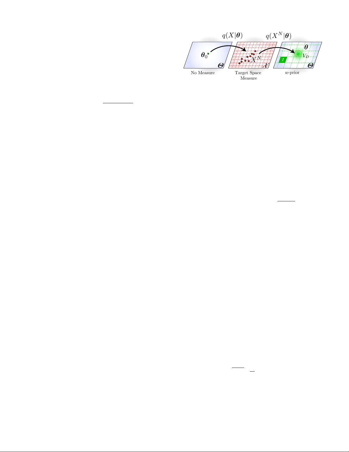
An objective prior that unifies objective Bayes and information-based inference. Colin H. LaMont and Paul A. W iggins Departments of Physics, Bioengineering and Microbiology , University of Washington, Box 351560. 3910 15th A venue Northeast, Seattle, W A 98195, USA ∗ There ar e three principle paradigms of statistical inference: (i) Bayesian, (ii) information-based and (iii) frequentist inference [ 1 , 2 ]. W e describe an objective prior (the weighting or w -prior) which uni- fies objective Bayes and information-based inference. The w -prior is chosen to make the marginal probability an unbiased estimator of the predictive performance of the model. This definition has several other natural interpretations. From the perspective of the information content of the prior , the w -prior is both uniformly and maximally uninformative. The w -prior can also be understood to result in a uniform density of distinguishable models in parameter space. Finally we demonstrate the the w -prior is equivalent to the Akaike Information Criterion (AIC) for regular models in the asymptotic limit. The w -prior appears to be generically applicable to statistical infer ence and is free of ad hoc regularization. The mechanism for suppressing complexity is analogous to AIC: model complexity reduces model predictivity . W e expect this new objective-Bayes approach to inference to be widely- applicable to machine-learning problems including singular models. P ACS numbers: Introduction. A long-standing goal of statistical infer- ence is the formulation of a consistent and generally- applicable objective-Bayes methodology [ 3 ]. Although the Bayes law formally depends on knowledge of a prior probability distribution (prior), from its infancy , Bayesian analysis has been applied in scenarios where this prior information is unknown [ 4 , 5 ]. A second prin- ciple paradigm of inference has been developed ar ound a frequentist formulation of probability , beginning with the work of C. F . Gauss, R. A. Fisher , etc [ 6 ]. In the 1970s, a third paradigm of information-based inference was developed based on the pioneering work of Akaike [ 7 – 9 ]. Although it is often possible to arrive at simi- lar conclusions using these distinct statistical paradigms [ 10 ], this is not always the case [ 4 , 11 ]. Summary . W e motivate the form of the w -prior using the Principle of Indiffer ence . W e propose a precise im- plicit definition of the w -prior by defining a Bayes pr edic- tive multiplicity : the number of indistinguishable models in the vicinity of parameterization θ . The w -prior has unit multiplicity for all model parameterizations. W e demonstrate that the resulting Bayes partition function is an unbiased estimator for the predictive performance of the learning machine. Next we show that the mul- tiplicity can be understood as the parameter-coding in- formation and using this formulation, we demonstrate that the w -prior is both uniformly and maximally unin- formative. Having established that the w -prior has many of the desired properties of an objective prior , we explore the connection to the information-based paradigm of statis- tical inference. W e demonstrate that for regular models [ 41 ], objective-Bayes inference is asymptotically equiv- ∗ Electronic address: pwiggins@uw .edu ; URL: http://mtshasta. phys.washington.edu/ alent to the Akaike Information Criterion (AIC) [ 7 – 9 ], unifying objective-Bayes and information-based infer- ence. Finally , we discuss predictivity as the unifying prin- ciple that is common to all three principle paradigms of inference. Preliminaries. W e introduce the following notation for a set of N independent and identically distributed ob- servations [ 42 ]: X N ≡ ( X 1 , X 2 , ..., X N ) where X i ∼ q ( ·| θ 0 ) , (1) and the distribution function q is parameterized by θ 0 , the true parameterization. W e model the probability dis- tribution with a set of model parameterizations θ ∈ Θ . In general this set will include models of different di- mension (i.e. complexity K ≡ dim θ ). W e assume a frequentist realization of Bayesian statistics: There are many realizations of the system of interest and the true parameterization is a random variable with a distribu- tion defined by the true prior distribution θ 0 ∼ $ 0 ( · ) . This true prior may or may not be known. W e intr oduce a generalizated marginal probability called the Bayes partition function [ 12 ]: Z ( X N | ρ ) ≡ Z Θ d θ ρ ( θ ) q ( X N | θ ) , (2) where ρ ( θ ) is a density of models on the manifold Θ that need not be normalized. When ρ = $ 0 , the marginal probability (partition function) has the meaning proba- bility of observing X N for an unknown true parameter- ization. The generalized posterior probability is defined: ρ ( θ | X N ) ≡ q ( X N | θ ) ρ ( θ ) Z ( X N | ρ ) , (3) which is known as the Bayes Law if ρ = $ 0 . Like the partition function, we generalize the posterior to permit 2 updating of any distribution on Θ . In this generalized case, the posterior is understood to have the meaning of a model weighting. Only when the posterior is con- structed with the true prior is the posterior understood as the probability distribution for the unknown true pa- rameterization, updated by the observations X N . Note that even if the prior is initially improper (unnormal- ized), the posterior will be normalized. The Bayes predictive distribution is defined: q ( X | X N , ρ ) ≡ Z ( X, X N | ρ ) Z ( X N | ρ ) , (4) where X / ∈ X N and is understood to be the Bayesian predicted probability distribution for a new observation X given N observations X N and a prior ρ . W e define the Bayesian free energy [ 12 ]: G ( X N , ρ ) ≡ − log Z ( X N | ρ ) (5) and the closely related performance estimator : P N post ( θ , ρ ) ≡ E X q ( ·| θ ) log Z ( X N | ρ ) . (6) The significance of this definition and its interpretation as an estimator will be discussed shortly . Finally we introduce the natural measure of predic- tive performance: the ability of the trained Bayes model to pr edict new observations. Again it is convenient to formulate the performance of the model for N new ob- servations. W e define the predictivity : P N pre ( θ , ρ ) ≡ N E X q ( ·| θ ) log q ( X | X N , ρ ) , (7) where X / ∈ X N . The predictivity is the Bayesian pr edic- tive performance for N simultaneous measurements. Principle of Indifference. In instances where no prior information was known, both P . S. Laplace [ 5 ] and T . Bayes [ 13 ] invoked a principle of indifference which assigned mutually exclusive and exhaustive possibilities equal prior probability [ 14 , 15 ]. Although this approach does lead to consistent results in the context of models with discrete parameterization, it has long been unclear how to generalize the principle of indiffer ence to a con- tinuum context where the meaning of both mutually ex- clusive and exhaustive are uncertain. The prior depends on N . In the interest specificity , con- sider the set of gaussian distributions with mean µ ∈ R and variance v = 1 . W e can write θ ≡ ( µ, v ) . Are two models with µ 1 6 = µ 2 mutually exclusive? Intuitively we know the answer: If the difference in the means is suf- ficiently small, we cannot distinguish the models for a small number of observations. But, whatever the values of the means µ i , if µ 1 6 = µ 2 then a sufficient number of observations N can always resolve the models, render - ing them mutually exclusive. Therefor e it is natural to X N θ 0 Θ Θ X q ( X | θ ) q ( X N | θ ) θ No Measure Target Space Measure w -prior 1 V D FIG. 1: Geometry of inference. Panel A: Inference defines a natural measure on parameter space Θ . T o understand the origin of this measure, consider a true parameterization θ 0 used to generate observations X N . W e then define a cutoff divergence D D to determine a region of indistinguishability on Θ with volume V D ( θ ) . W e define the density of models as ρ D ≡ V − 1 D . assume that the condition for model distinguishability depends on the number of observations. Estimating the density of models. V . Balasubramanian and others [ 16 ] have argued that a natural measure for testing distinguishability for θ 1 6 = θ 2 exists and is given by the KL Divergence [ 17 , 18 ]: D ( θ 1 || θ 2 ) ≡ Z X d x q ( x | θ 1 ) log q ( x | θ 1 ) q ( x | θ 2 ) , (8) which is a measure of distance between any two proba- bility distributions. For θ 1 = θ 2 , the divergence is iden- tically zero and D > 0 for q ( x | θ 1 ) 6 = q ( x | θ 2 ) [ 17 , 18 ]. For simplicity , assume that we pick some critical value of the divergence D D , below which two distributions are considered indistinguishable ( ∼ D ) and above which two distributions are distinguishable (  D or mutually exclu- sive ). The sum over equally weighted mutually exclu- sive distributions can be written as an integral [ 16 ]: X  D − → Z Θ d θ ρ D ( θ ) , (9) where ρ − 1 D = V D is the parameter-space volume of pa- rameterizations that are equivalent in the vicinity of θ . (For the moment, assume all θ ∈ Θ are continuous pa- rameters of dimension K . A schematic drawing of the meaning of the parameter-space volume is illustrated in Fig. 1 .) The divergence for N observations is simply N times the divergence for one. For a large number of ob- servations N and a regular model, we can write the den- sity of distinguishable model as [ 16 ]: ρ D ∝ √ det I  N 2 π  K/ 2 D − K/ 2 D , (10) where I is the Fisher Information Matrix [ 19 ]. Clearly this density is increasing in N since the resolution of the learning machine increases with the number obser- vations. The canonical approach is to drop the N de- pendence, keeping only the determinant in the Fisher 3 Information Matrix [ 16 ]. But for the purpose of count- ing distinguishable models with distinct dimension K , it is essential to retain the N dependence since it cannot be factored out of the sum in Eqn. 9 . W e will make a more pr ecise definition of the density of models shortly , but the insistence that the prior (the density of models) depends on the number of observa- tions N has profound consequences as we describe be- low . Note that for fixed model dimension K , we will show that Eqn. 10 is correct for a specific value of the criti- cal divergence D D . One might hope that inference was either independent or weakly dependent on D D but in fact its value is critically important. W e therefor e need to propose a more precise definition of the density of models. The multiplicity and the w -prior . T o define the density of models precisely , we first intr oduce the Bayes predic- tive multiplicity m : log m ( θ 0 , ρ ) ≡ P N post ( θ 0 , ρ ) − P N pre ( θ 0 , ρ ) . (11) The meaning of the multiplicity is the number of indis- tinguishable models defined by the prior in the vicinity of θ 0 . (W e will return to this discussion shortly .) W e define the weighting prior ( w -prior) as the density of indistinguishable models such that the multiplicity is unity for all true models in the set Θ : m ( θ 0 , w ) = 1 ∀ θ 0 ∈ Θ . (12) Clearly w will in general be an improper prior . The name “weighting” is chosen to emphasize the model- weighting rather than probabilistic interpretation of anal- ysis as described below [ 8 ]. An unbiased estimator of performance. For an im- proper prior , the partition funciton can no longer be understood as the marginal probability of observations X N . But the definition of the w -prior gives the partition function a pr ecise mathematical meaning: Eqn. 11 , eval- uated at the w -prior (Eqn. 12 ), implies that the perfor- mance estimator (Eqn. 6 ) and by extension the log parti- tion function (Eqn. 2 ) ar e unbiased estimators [ 8 , 20 ] of the predictive performance of the model (Eqn. 7 ). Therefor e the partition function is understood as the pr obability of the last N measurements in the subjective-Bayes frame- work, but as an estimate of the pr obability of the next N in the objective-Bayes framework. Connection to the Gibbs Entropy . T o understand the mathematical meaning of the multiplicity m (Eqn. 11 ), it is helpful to transform the equation to write it in terms of the posterior probability distribution. W e an- alytically continue the number of observations to define the continuous variable effective temperature : T ≡ N − 1 (e.g. [ 12 ]). W e can now identify the definition of the mul- tiplicity as exactly analogous to the computation of the disorder -averaged Gibbs entropy ( S ) (e.g. [ 21 , 22 ]): S ( T , ρ, θ 0 ) ≡ − ∂ T F = log m + O ( T ) , (13) from the disor der-averaged Helmholtz free ener gy ( F ): F ( T , ρ, θ 0 ) ≡ − T h log Z i X , (14) where the angle brackets repr esent the expectation over X N with respect to the true distribution parameterized by θ 0 and the order T corr ection is an error due to the analytic continuation of the number of observations N [ 23 ]. In a physical context, X N is quenched disor- der [ 16 ]. The w -prior satisfies the condition that the disorder -averaged Gibbs entropy is zero to or der 1 N : S ( 1 N , w , θ 0 ) = 0 + O ( 1 N ) , (15) for all θ 0 ∈ Θ . The meaning of multiplicity . Re-expressing Eqn. 13 in statistical quantities gives the following expression for the multiplicity: log m ( θ 0 , ρ ) = E X,Y q ( ·| θ 0 ) E θ ρ ( ·| Y N ) log ρ ( θ ) ρ ( θ | X N ) + O ( 1 N ) . (16) The meaning of the multiplicity is understood as fol- lows: θ can be understood as the estimator of θ 0 . ρ ( θ ) is the density of models at θ and V D ≈ ρ − 1 ( θ | X N ) is the parameter-space volume of indistinguishable mod- els. Therefore the multiplicity m is the number of indis- tinguishable models defined by the prior ρ ( θ ) . See Fig. 1 for a schematic illustration. Although this expression is almost in the form of the divergence, the expectation is taken over the posterior probability distribution for an independent dataset Y N . This cross-validation form is a key distinction and avoids the over-fitting phenomena [ 43 ]. The parameter-coding interpretation. W e now wish to re-interpr et the multiplicity as a parameter-coding in- formation. W e define the parameter -coding information content of the observations: H θ ( θ 0 , $ ) ≡ E X,Y q ( ·| θ 0 ) E θ $ ( ·| X N ) log $ ( θ | Y N ) $ ( θ ) , (17) given a normalized prior $ . Note that as before we are careful to define the parameter-coding information by cross-validation as before with posterior probability dis- tributions generated from independent datasets X N and Y N . W e now need to define a normalized w -prior . W e inte- grate overall parameter space (applying a cutoff if nec- essary) to determine the normalization constant (total number of models): N Θ ≡ Z Θ d θ w ( θ ) . (18) W e define the normalized w -prior: $ w ≡ N − 1 Θ w [ 44 ]. Inserting the normalized w -prior into the parameter- coding information gives H θ ( θ 0 , $ w ) = log N Θ + O ( 1 N ) , (19) 4 which is clearly constant with respect to the true model θ 0 up to order 1 N . The w -prior is uniformly uninformative. W e now wish to analyze the dependence of the average parameter- coding information H θ on the true model θ 0 . Informa- tive priors have the property that they code informa- tion about the underlying true model. A prior localized around the true value θ 0 will reduce the information content of the observations. Therefore we might intu- itively expect an uninformative prior to result in a con- stant information content with r espect to the true model θ 0 . The w -prior has this property to or der 1 N . No pa- rameter values are favored or disfavored. W e therefore say that the w -prior is uniformly uninformative since the information gain is independent of the true model. The w -prior is maximally uninformative. In the def- inition of the refer ence prior , J. M. Bernardo argued that an objective and uninformative prior should maxi- mize the information specified by the observations [ 24 ]. W e therefore construct an expression analogous to that which he proposed, differing only in the use of the cross- validation form of the parameter-code information: H θ ( $ ) ≡ E θ $ H θ ( θ , $ ) , (20) which can be understood as the expectation of the H θ ( θ , $ ) over a true prior $ . A prior which is maxi- mally uninformative, should be stationary with respect to variations in the prior . $ w is stationary and a least locally a maximum to order N − 1 . W e therefor e con- clude that the w -prior also possesses the property that it is maximally uninformative . The w -prior for a regular model. In general, there is no closed-form expr ession of the w -prior although it can be computed exactly for a number of special cases and for sufficiently simple models [ 23 ]. In the interest of simplicity consider a regular model where the number of continuous degrees of freedom in the model parameterization θ is K and work in the large number of observations N limit. Using the Gibbs en- tropy equation for the w -prior , we compute the w -prior [ 23 ]: w ( θ ) = J  N 2 π  K/ 2 e − K , (21) where J ( θ ) ≡ √ det I , (22) is equal to the square root of the determinant of the Fisher Information Matrix and is the well known Jef- freys prior that H. Jeffr eys proposed to insure invariance of the probability to re-parameterization of θ [ 25 , 26 ]. It is instructive to immediately compare this results to form we estimated based on principle of indifference (Eqn. 10 ). These arguments correctly identified both the Jeffr eys prior factor J and the scaling with the number of observations N . But, a precise formulation was re- quired to correctly compute the last factor in Eqn. 21 , the penalty e − K , which plays a critical role in the reg- ularization of the w -prior when the complexity of the model is unknown. Clearly Eqn. 21 implies that for any significant num- ber of observations N , the w -prior appears to incr ease with model complexity K , but all factors except the for e − K cancel during mar ginalization over θ in the compu- tation of the partition function (Eqn. 2 ). The qualitative understanding of the w -prior is therefore a penalization (regularization) of model complexity . Equivalence to information-based inference. W e now compute the w -prior for a regular model of unknown complexity K . T ypically for models of unknown com- plexity , the w -prior cannot be computed exactly . W e have therefor e developed a recursive technique [ 23 ] analogous to that proposed by J. M. Bernardo [ 24 ]. W e write the total model parameterization as θ ≡ ( K, θ K ) where the θ K are K continuous parameters. The first- order expression for the w -prior for a regular model of unknown complexity is still given by Eqn. 21 with θ → θ K [ 23 ]. The partition function using the first-order expression for the w -prior is: Z = ∞ X K =1 Z K , (23) G K ≡ − log Z K = − log q ( X N | K, ˆ θ K X ) + K , (24) where the ˆ θ K X are the Maximum Likelihood Estimators of the parameters θ K , Z K and G K are the partition func- tion and free energy at complexity K . The first term in the free energy is the minus-log likelihood and the sec- ond term is interpreted as a penalization for model com- plexity . T o those familiar with the information-based ap- proach of Akaike, it is clear that the free energy G K is identical to AIC: G K = AIC K , (25) for a model with K degrees of freedom [ 7 , 8 ]. Ther e- fore, in the asymptotic limit for regular models, the w - prior will simply recover information-based inference [ 45 ]. The K penalty is the information-based realization of Occam’ s Razor : parsimony implies predictivity . The w -prior for singular models. Singular models con- tain parameters for which the Fisher Information is zero (or nearly zero for finite N ). AIC fails in the context of singular models but we have recently proposed a gener- alization of AIC called the Frequentist Information Cri- terion (FIC) for application to singular models [ 27 , 28 ], which is equivalent to Neyman-Pearson hypothesis test- ing [ 27 , 28 ]. Given the close connection between AIC and the w -prior described above, one might hope that w -prior for a singular model would be analogous to FIC. The equivalence between information-based inference and the w -prior appears to a hold only for r egular mod- els in the asymptotic limit ( N → ∞ ). It is well known 5 that Bayesian inference, corresponding to the Schwartz distribution topology , has a finite generalization error in the asymptotic limit, whereas maximum-likelihood- based techniques result in divergent generalization er- rors in the asymptotic limit (e.g. [ 12 ]). W e provide a de- tailed description of the connections between objective bayes, information-based and fr equentist inference else- where [ 23 , 27 ]. The weighting interpretation. The w -prior and poste- rior probability distribution for the model parameteri- zation θ should be understood as a model weighting , not as the probability density that θ is the true parameteriza- tion θ 0 . W e have given the w -prior the name of weighting prior in close analogy to the Akaike weights (e.g. [ 8 ]). From a fr equentist perspective, we are forbidden from discussing the probability of a model which we cannot compute since we do not know the prior from which the truth was constructed. The weighting interpretation is not simply philosophical point, but has important com- putational significance. For instance, as the number of observations N increases, the resolution of the objective- Bayes learning machine increases also and therefore as a consequence the weighting of more complex models in the w -prior increases also. As a result, the complex- ity of the fit model naturally increases with the size of the dataset when describing an infinite dimensional true model, as predicted by the information-based approach. The infinite complexity of the true model is of no conse- quence to the selection of the objective w -prior . Like subjective-Bayes inference, the w -prior generates a weighted ensemble of models rather than a point es- timate or confidence intervals and therefore has both the associated advantages and short-comings of the Bayesian machinery . A number of authors (e.g. [ 29 ]) have ar gued that the fr equentist approach is itself ad hoc due to the bewildering proliferation of tests and statis- tics. These authors may view the w -prior , not as a tool for Bayesian statisticians, but rather as a missing unify- ing principle for frequentist methods to place them on par with existing Bayesian methods. Cross-validation. Predictivity , cross-validation, boot- strapping and generalization error are all essentially mathematically equivalent measures of model perfor- mance [ 46 ]. Therefor e, clearly the w -prior can be in- terpreted to be weighted to optimize cross-validation or generalization-error -based measures of performance. In fact, it has recently been formally demonstrated that stability to cross-validation is a necessary and sufficient condition for the predictive performance of a learning machine [ 30 ]. The central role of predictivity . Motivated by the work of Akaike, we have repeatedly made use of the princi- ples of predictive performance . For instance, see Eqns. 11 , 17 and 27 . The critical consideration in each of these equations is always generalization : the model perfor- mance measured against data not included in the train- ing set. It is this formulation that leads to model selec- tion (or model regularization ). For instance, if one were to define the multiplicity (Eqn. 11 ) with respect to the postdictive performance [ 47 ] or even the performance of the true model [ 48 ], the w -prior could not be con- sistently defined for an infinitely-nestable model since there would be an ultraviolet divergence [ 31 ] for high- complexity (large K ) models. It is the use of the predic- tive performance as the model weighting that gives rise to regularization which is both natural and statistically- principled. It is unnecessary to augment the predictive regularization with exogenous and ad hoc regulatory de- vices such as smoothing [ 32 ], hyper-parameters [ 33 ] or vague priors [ 34 ]. The maximum-predictivity interpretation. Finally we wish to discuss our results in the context of subjective Bayes analysis where the true prior is known. W e note the true prior is optimal in two senses. (i) The true prior maximizes the expectation of the performance estimator (e.g. [ 12 ]): P N post ( $ 0 , $ ) ≡ E θ $ 0 P N post ( θ , $ ) , (26) which has a unique global maximum at $ = $ 0 . But with particular relevance to our current work, the true prior is also optimal in a predictive sense. (ii) The true prior maximizes the expectation of the predictivity (e.g. [ 12 ]): P N pre ( $ 0 , $ ) ≡ E θ $ 0 P N pre ( θ , $ ) , (27) which has a unique global maximum at at $ = $ 0 . It is tempting ask whether there is some prior that opti- mizes predictivity directly if the true prior is not know , in analogy to Eqn. 27 , but no such prior exists [ 12 , 23 ]. Discussion. W e have presented predictive performance as a unified framework for reconsiling the three princi- ple paradigms of statistical inference [ 1 , 2 ]. As discussed in the previous section, subjective-Bayesian analysis can be understood to directly maximize the predictive per- formance of the model if (and only if) the true prior is used to generate inference. But by far the most important practical scenario is an unknown true prior . In this cases, the predictive perfor- mance of the model cannot be strictly maximized since the true prior is unknown. In this scenario, we pro- pose that inference be performed by weighting models by their expected predictive performance using the w - prior . As we have demonstrated, the w -prior results in a partition function which is the unbiased estimator of model performance. Ther efore inference using the w - prior can also be understood as the optimization of pre- dictive performance, although not in the strict sense of maximization. The w -prior is improper and yet has a rigorous statis- tical meaning. There has been a long history of the suc- cessful application of impr oper priors in statistical anal- 6 ysis, most famously by H. Jeffr eys [ 25 ], and despite con- siderable, ongoing and heated debated about the statis- tical meaning and rigor of these approaches [ 33 , 35 – 37 ]. W e have proposed one possible rigorous definition for an improper prior and have described why such priors have good performance from a fr equentist perspective. The w -prior also has a natural interpretation as an uninformative prior . (i) It is a realization of the Princi- ple of Indifference in the sense that the prior weights all distinguishable models equally . Since this scenario de- scribes a state of maximum entropy , the w -prior has a MaxEnt interpretation. (ii) It is uniformly uninformative in the sense the parameter-information content of the observations is independent of the true model. (iii) It is maximally uninformative in the sense that it maximizes the model-averaged parameter-information content of observations and can therefor e be interpreted as a ref- erence prior . Finally we demonstrated that the w -prior is equivalent to information-based AIC infer ence for regu- lar models. The w -prior has virtually all of the desirable properties of an objective-Bayesian prior with one key short-coming: Both the prior and the posterior have a weighting rather than a Bayesian probabilistic interpre- tation. W e believe that such an interpretation is not only philosophically desirable but a mathematical necessity . [1] P . S. Bandyopadhyay and M. R. Forster . Handbook of the Philosophy of Science: Philosophy of Statistics , volume 7, chapter 3. Elsevier , 2011. [2] W ikipedia. Statistical inference — wikipedia, the free en- cyclopedia, 2015. [Online; accessed 22-April-2015] . [3] J. O. Berger . The case for objective bayesian analysis. Bayesian Analysis , 1(3):385–402, 2006. [4] H. Jeffr eys. The theory of probability . Oxfor d University Press, 1939. [5] P . S. Laplace. Theorie analytique des probabilites. . Courcier Imprimeur , Paris, 3rd edition, 1812. [6] D. R. Cox. Proceedings of PHYST A T05: Statistical Problems in Particle Physics, Astrophysics and Cosmology , chapter Fre- quentist and bayesian statistics: A critique., pages 3–6. 2005. [7] H. Akaike. Information theory and an extension of the maximum likelihood principle. In Petrov B. N. and E. Csaki, editors, 2nd International Symposium of Informa- tion Theory . , pages 267–281. Akademiai Kiado, Budapest., 1973. [8] K. P . Burnham and D. R. Anderson. Model selection and multimodel inference. Springer-V erlag New Y ork, Inc., 2nd. edition, 1998. [9] W ikipedia. Akaike information criterion — wikipedia, the free encyclopedia, 2015. [Online; accessed 22-April- 2015] . [10] M. J. Bayarri and J. O. Berger . The interplay between bayesian and frequentist analysis. Statistical Science. , 19:58–80, 2004. [11] W ikipedia. Lindley’s paradox — wikipedia, the free en- cyclopedia, 2015. [Online; accessed 23-April-2015] . [12] S. W atanabe. Algerbraic geometry and statistical learning the- ory . Cambridge Univeristy Press, 2009. [13] T . Bayes. An essay toward solving a problem in the doc- trine of chances. Phil. T rans. Roy. Soc. , 53 54:370–418 296– 325. [14] J. M. Keynes. A T reatise on Probability . Macmillan Limited, London, 1921. [15] W ikipedia. Principle of indifference — wikipedia, the free encyclopedia, 2014. [Online; accessed 22-April-2015] . [16] V . Balasubramanian. Statistical inference, occam’s razor , and statistical mechanics on the space of probability dis- tributions. Neural Computation , 9:349–368, 1997. [17] S. Kullback and R.A. Leibler . On information and suffi- ciency . Annals of Mathematical Statistics , 22:79–86, 1951. [18] W ikipedia. Kullback–leibler diver gence — wikipedia, the free encyclopedia, 2015. [Online; accessed 22-April-2015] . [19] W ikipedia. Fisher information — wikipedia, the free en- cyclopedia, 2015. [Online; accessed 22-April-2015] . [20] W ikipedia. Bias of an estimator — wikipedia, the free en- cyclopedia, 2015. [Online; accessed 22-April-2015] . [21] F . Reif. Statistical Physics. McGraw-Hill (New Y ork), 1967. [22] W ikipedia. Entropy (statistical thermodynamics) — wikipedia, the free encyclopedia, 2015. [Online; accessed 22-April-2015] . [23] Colin H. LaMont and Paul A. W iggins. A detailed de- scription of the w -prior . In preparation , 2015. [24] J. O. Berger and J.-M. Bernardo. On the development of the reference prior method. T echincal Report 91-15C, Pur - due University , 1991. [25] H. Jeffreys. An invariant form for the prior probabil- ity in estimation problems. Proceedings of the Royal Soci- ety of London. Series A, Mathematical and Physical Sciences , 186(1007):453–461, 1946. [26] W ikipedia. Jef freys prior — wikipedia, the free encyclo- pedia, 2015. [Online; accessed 22-April-2015] . [27] Colin H. LaMont and Paul A. W iggins. The fr equentist in- formation criterion (FIC): The unification of information- based and frequentist infer ence. In preparation. , 2015. [28] Paul A. W iggins. A simple application of the frequentist information criterion (FIC) to model selection. In prepara- tion. , 2015. [29] T . J. Loredo. Maximum-Entr opy and Bayesian Methods , chapter From Laplace to Supernova SN 1987A: Bayesian Inference in Astrophysics, pages 81–142. Dartmouth, Dor- drecht, The Netherlands: Kluwer Academic Publishers, 1990. [30] T . Poggio, R. Rifkin, S. Mukherjee, and P . Niyogi. Gen- eral conditions for pr edictivity in learning theory . Nature , 428(6981):419–22., 2004. [31] W ikipedia. Ultraviolet divergence — wikipedia, the free encyclopedia, 2015. [Online; accessed 22-April-2015] . [32] D. J. C. MacKay . Bayesian interpolation. Neural Computa- tion , 4(3):415–447, 1992. [33] D. J. C. MacKay . Information Theory, Inference, and Learning Algorithms. Cambridge Univeristy Press, 2003. [34] R. E. Kass and A. E. Raftery . Bayes factors. Journal of the American Statistical Association , 90(430):773–795, 1995. [35] A. P . Dawid, M. Stone, and J. V. Zidek. Marginaliza- tion paradoxes in bayesian and structural inference with 7 discussion. J Roy Statist Soc B , 35:189–233, 1973. [36] A. P . Dawid, M. Stone, and J. V. Zidek. Bayesian Analysis in Econometrics and Statistics , volume 35, chapter Comments on Jayness pap er MarginalŁ ization and prior probabilities, pages 189–233. NorthŁ Holland Co, Ams- terdam, 1973. [37] E. T . Jaynes. Probability Theory: The Logic of Science. Cam- bridge University Press., 2003. [38] G. E. Schwarz. Estimating the dimension of a model. An- nals of Statistics , 6(2):461–464, 1978. [39] W ikipedia. Bayesian information criterion — wikipedia, the free encyclopedia, 2015. [Online; accessed 22-April- 2015] . [40] Kenneth P . Burnham and David R. Anderson. Multi- model inference: Understanding AIC and BIC in model selection. Socialogical Methods & Research , 33(2):261–304, 2004. [41] A model is regular if the eigenvalues of the Fisher In- formation Matrix are large enough to make the log- likelihood effectively harmonic in the parameter values around their MLE or MAP value. [42] When X appears in upper case, it should be understood as a random variable whereas it is a normal variable when it appears in lower case. If we need a statistically indepen- dent set of variables of equal size, we will use the random variables Y N , which have identical pr operties to the X N . [43] Note that this cr oss-validation is virtual . No explicit cr oss- validation will be performed on true data. [44] Note that regar dless of whether N θ is strictly conver gent, the multiplicity is well defined. Only our interpretation as a parameter-coding information is dependent of regu- larizing N Θ . [45] In fact in the context of discussing the connection between the Bayesian Information Criterion (BIC) [ 8 , 38 , 39 ] and AIC, K. Burnham and D. Anderson suggested that just such a prior would be a savvy prior due to its good fre- quentist attributes [ 40 ]. [46] These measures are equivalent for a large number of ob- servations N . [47] Postdiction: The performance of the model in repr oduc- ing the training set. [48] J.-M. Bernardo has proposed a somewhat analogous prior , the refer ence prior , which uses the true model as the refer ence in the multiplicity (e.g. [ 24 ]). This approach has exactly the shortcomings one would predict. The prior is not consistent for nested models.