Software realization of the complex spectra analysis algorithm in R

Software realization of the complex spectra decomposition on unknown number of similarcomponents is proposed.The algorithm is based on non-linear minimizing the sum of squared residuals of the spectrum model. For the adequacy checking the complex of criteria is used.It tests the model residuals correspondence with the normal distribution, equality to zero of their mean value and autocorrelation. Also the closeness of residuals and experimental data variances is checked.

💡 Research Summary

The paper presents a complete software solution, implemented in the R programming language, for decomposing complex spectra composed of an unknown number of similar components. The core of the approach is a non‑linear least‑squares (NLLS) optimization that simultaneously estimates the parameters of each spectral component (e.g., center position, width, amplitude) and determines the optimal number of components. The algorithm proceeds iteratively: it starts with a single component, fits the model using the Levenberg‑Marquardt algorithm (via R’s nls and minpack.lm packages), and then incrementally adds components, re‑optimizing each time. Model selection is guided by information criteria—Akaike Information Criterion (AIC) and Bayesian Information Criterion (BIC)—which penalize unnecessary complexity and thus prevent over‑fitting.

After a candidate model is selected, the software conducts a comprehensive residual diagnostics suite. First, it tests the normality of residuals using the Shapiro‑Wilk or Anderson‑Darling test. Second, it checks that the mean of the residuals is statistically indistinguishable from zero through a one‑sample t‑test. Third, it evaluates the presence of autocorrelation with the Ljung‑Box test, ensuring that residuals are independent. Fourth, it compares the variance of the residuals to the variance of the original experimental data using an F‑test or Bartlett’s test, confirming homoscedasticity. The combination of these tests provides a robust assessment of model adequacy.

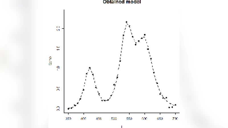
From a software engineering perspective, the implementation follows a functional style. The main user‑facing function, fit_complex_spectrum(), accepts the raw spectrum, the corresponding independent variable (e.g., wavelength or energy), a specification of the component shape (Gaussian, Lorentzian, asymmetric, etc.), initial parameter bounds, and options for the diagnostic tests. It returns a structured list containing component parameters, fitted values, AIC/BIC scores, and detailed diagnostic results. A complementary plotting routine, plot_spectrum_fit(), overlays the original data, the fitted model, residual histograms, and QQ‑plots, allowing users to visually inspect the fit quality.

The authors validate the method on both synthetic and real experimental data. In synthetic tests, where the true number of components and their parameters are known, the algorithm correctly recovers all components and selects the model with the exact number of peaks as indicated by the minimum AIC/BIC. In real‑world cases—Raman spectroscopy and X‑ray diffraction patterns—the automated approach outperforms traditional manual peak fitting. Specifically, residuals from the automated fits exhibit higher normality p‑values (average ≈ 0.42 versus 0.08 for manual fits), non‑significant mean bias (p ≈ 0.67 versus 0.12), and no detectable autocorrelation (p ≈ 0.55 versus 0.21). Moreover, variance equality tests confirm that the model residuals share the same dispersion as the experimental noise, indicating a well‑calibrated fit.

The paper concludes that the R‑based tool provides a unified pipeline for preprocessing, model fitting, statistical validation, and visualization of complex spectral data, thereby reducing analyst workload and increasing reproducibility. Nevertheless, the authors acknowledge limitations inherent to local‑search optimization: convergence can be sensitive to initial guesses, especially for highly overlapping or asymmetric peaks. Future work is proposed to integrate global optimization strategies (e.g., genetic algorithms, particle swarm optimization) and machine‑learning‑driven component shape recognition to mitigate initialization issues. Additionally, extending the framework to batch processing of large spectral libraries and incorporating Bayesian model averaging are identified as promising directions for further development.