Learning Scale-Free Networks by Dynamic Node-Specific Degree Prior

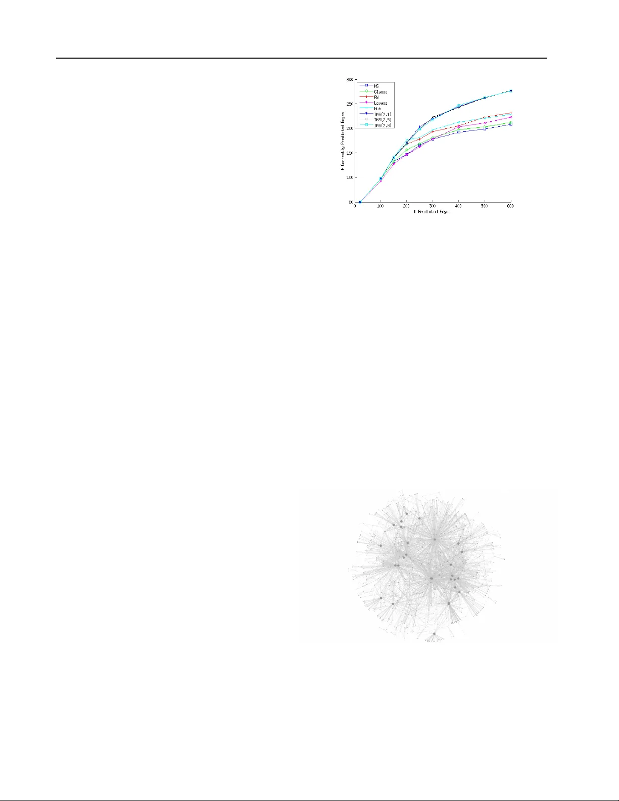
Learning Scale-Fr ee Networks by Dynamic Node-Specific Degr ee Prior Qingming T ang 1 Q M TAN G @ T T I C . E D U T oyota T echnological Institute at Chicago, 6045 S. Kenwood A ve., Chicago, Illinois 60637, USA Siqi Sun 1 S I Q I @ T T I C . E D U T oyota T echnological Institute at Chicago, 6045 S. Kenwood A ve., Chicago, Illinois 60637, USA Jinbo Xu J I N B O . X U @ G M A I L . C O M T oyota T echnological Institute at Chicago, 6045 S. Kenwood A ve., Chicago, Illinois 60637, USA Abstract Learning network structure underlying data is an important problem in machine learning. This pa- per presents a nov el de gree prior to study the in- ference of scale-free networks, which are widely used to model social and biological networks. In particular , this paper formulates scale-free net- work inference using Gaussian Graphical model (GGM) regularized by a node degree prior . Our degree prior not only promotes a desirable global degree distribution, but also e xploits the esti- mated degree of an individual node and the rela- tiv e strength of all the edges of a single node. T o fulfill this, this paper proposes a ranking-based method to dynamically estimate the degree of a node, which makes the resultant optimization problem challenging to solve. T o deal with this, this paper presents a novel ADMM (alternating direction method of multipliers) procedure. Our experimental results on both synthetic and real data show that our prior not only yields a scale- free network, but also produces many more cor- rectly predicted edges than existing scale-free in- ducing prior , hub-inducing prior and the l 1 norm. 1. Introduction Graphical models are widely used to describe the rela- tionship between variables (or features). Estimating the structure of an undirected graphical model from a dataset has been extensi vely studied ( Meinshausen & B ¨ uhlmann , 1 Equal Contribution. Pr oceedings of the 32 nd International Confer ence on Machine Learning , Lille, France, 2015. JMLR: W&CP volume 37. Copy- right 2015 by the author(s). 2006 ; Y uan & Lin , 2007 ; Friedman et al. , 2008 ; Banerjee et al. , 2008 ; W ainwright et al. , 2006 ). Gaussian Graph- ical Models (GGMs) are widely used to model the data and l 1 penalty is used to yield a sparse graph structure. GGMs assume that the observed data follows a multiv ari- ate Gaussian distribution with a covariance matrix. When GGMs are used, the network structure is encoded in the zero pattern of the precision matrix. Accordingly , struc- ture learning can be formulated as minimizing the nega- tiv e log-likelihood (NLL) with an l 1 penalty . Howe ver , the widely-used l 1 penalty assumes that any pair of variables is equally likely to form an edge. This is not suitable for many real-world networks such as gene networks, protein- protein interaction networks and social networks, which are scale-free and contain a small percentage of hub nodes. A scale-free netw ork ( B ARAB ´ ASI & Bonabeau , 2003 ) has node degree following the power -law distribution. In par- ticular , a scale-free network may contain a few hub nodes, whose degrees are much larger than the others. That is, a hub node more likely forms an edge than the others. In real-world applications, a hub node is usually functionally important. For example, in a gene network, a gene playing functions in many biological processes ( Zhang & Horvath , 2005 ; Goh et al. , 2007 ) tends to be a hub . A few methods hav e been proposed to infer scale-free networks by using a reweighed l 1 norm. For example, ( Peng et al. , 2009 ) pro- posed a joint regression sparse method to learn scale-free networks by setting the penalty proportional to the esti- mated degrees. ( Candes et al. , 2008 ) proposed a method that iterativ ely reweighs the penalty in the l 1 norm based on the inv erse of the pre vious estimation of precision ma- trix. This method can suppress the large bias in the l 1 norm when the magnitude of the non-zero entries vary a lot and is also closer to the l 0 norm. Some recent papers follo w the idea of node-based learning using group lasso ( Friedman et al. , 2010b ; Meier et al. , 2008 ; T an et al. , 2014 ; Fried- man et al. , 2010a ; Mohan et al. , 2014 ). Since group lasso Learning Scale-Fr ee Networks by Dynamic Node-Specific Degree Prior penalty promotes similar patterns among variables in the same group, it tends to strengthen the signal of hub nodes and suppress that of non-hub nodes. As such, group lasso may only produce edges adjacent to nodes with a large de- gree (i.e., hubs). In order to capture the scale-free property , ( Liu & Ihler , 2011 ) minimizes the negati ve log-likelihood with a scale- free prior , which approximates the degree of each variable by the l 1 norm. Howe ver , the objective function is non- con vex and thus, is hard to optimize. ( Defazio & Caetano , 2012 ) approximates the global node degree distribution by the submodular con vex en velope of the node degree func- tion. The con vex env elope is the Lovasz extension ( Lov ´ asz , 1983 ; Bach , 2010 ) of the sum of logarithm of node de gree. These methods consider only the global node de gree distri- bution, but not the degree of an individual node. Howe ver , the approximation function used to model this global de- gree distribution may not induce a power -law distribution, because there are many possible distributions other than power -law that optimizing the approximation function. See Theorem 1 for details. T o further improve scale-free network inference, this pa- per introduces a nov el node-degree prior , which not only promotes a desirable global node degree distribution, but also e xploits the estimated degree of an individual node and the relative strengths of all the edges adjacent to the same node. T o fulfill this, we use node and edge ranking to dy- namically estimate the de gree of an indi vidual node and the relativ e strength of one potential edge. As dynamic ranking is used in the prior , the objectiv e function is very challeng- ing to optimize. This paper presents a no vel ADMM (alter - nating direction method of multipliers) ( Boyd et al. , 2011 ; Fukushima , 1992 ) method for this. 2. Model 2.1. Notation & Preliminaries Let G = ( V , E ) denote a graph, where V is the verte x set ( p = | V | ) and E the edge set. W e also use E to de- note the adjacency matrix of G , i.e., E ij = 1 if and only if ( i, j ) ∈ E . In this paper we assume that the variable set V has a Gaussian distribution with a precision matrix X . Then, the graph structure is encoded in the zero pat- tern of the estimated X , i.e. the edge formed by X is E ( X ) = { ( u, v ) , X uv 6 = 0 } . Let F ( X ) denote the objec- tiv e function. For GGMs, F ( X ) = tr ( X S ) − log det( X ) , where S is the empirical covariance matrix. T o induce a sparse graph, a l 1 penalty is applied to obtain the following objectiv e function. ˆ X = arg min X F ( X ) + λ k X k 1 (1) Here we define two ranking functions. For a giv en i , let ( . ) denote the permutation of (1 , 2 , ..., p − 1) such that | X i, (1) | ≥ | X i, (2) | ≥ ... ≥ | X i, ( p − 1) | where ( X i, (1) , X i, (2) , ..., X i, ( p − 1) ) is a shuf fle of a row v ector X i excluding the element X i,i . Let M be a p − 1 dimension positiv e vector and V a p dimension vector . W e define X i ◦ M = P p − 1 u =1 | X i, ( u ) | M u . Let [ X, M , V ] be a per- mutation of (1 , 2 , ..., p ) such that X [1 ,X,M ,V ] ◦ M + V 1 ≥ X [2 ,X,M ,V ] ◦ M + V 2 ≥ ... ≥ X [ p,X,M ,V ] ◦ M + V p , where [ j, X, M , V ] denote the j th element of [ X , M , V ] . When V is a zero vector , we also write [ X, M , V ] as [ X , M ] and [ j, X, M , V ] as [ j, X , M ] , respecti vely . T o promote a sparse graph, a natural way is to use a l 1 penalty to regulate F ( X ) . Howe ver , l 1 norm cannot in- duce a scale-free network. This is because that a scale-free network has node degree following a power -law distribu- tion, i.e., P ( d ) ∝ d − γ where d is the degree and γ is a constant ranging from 2 to 3, rather than a uniform distri- bution. A simple prior for scale-free networks is the sum of the logarithm of node degree as follo ws. λ p X v =1 γ log( d v + 1) , (2) where d v = P p u =1 I [ X v u 6 = 0 , u 6 = v ] and I is the indi- cator function. The constant 1 is added to handle the situa- tion when d v = 0 . The l 0 norm in ( 2 ) is non-differentiable and thus, hard to optimize. One way to resolve this prob- lem is to approximate d v by the l 1 norm of X v as shown in ( Liu & Ihler , 2011 ). Since the logarithm of l 1 approx- imation is non-conv ex, a con vex en velope of ( 2 ) based on submodular function and Lovasz e xtension ( Lov ´ asz , 1983 ) is introduced recently in the papers ( Bach , 2010 ; Defazio & Caetano , 2012 ) as follows. p X v =1 p − 1 X u =1 | X v , ( u ) |  log( u + 1) − log( u )  . (3) Let h ( u ) = (log( u + 1) − log( u )) . The conv ex en velope of Eq. 2 can be written as p X v =1 p − 1 X u =1 h ( u ) | X v , ( u ) | . (4) 2.2. Node-Specific Degree Prior Although Eq. 2 and its approximations can be used to in- duce a scale-free graph, they still hav e some issues, as ex- plained in Theorem 1 . Theorem 1. Let S ( G ) denote the sum of logarithm of node de gr ee of a graph G . F or any graph G satisfying the scale- fr ee pr operty , ther e exists another graph G 0 with the same number of edges but not satisfying the scale-free pr operty such that S ( G 0 ) < S ( G ) . Learning Scale-Fr ee Networks by Dynamic Node-Specific Degree Prior Since we would like to use ( 2 ) as a regularizer , a smaller value of ( 2 ), denoted as S ( G ) , is always fav orable. Here we briefly prove Theor em 1 . Since G is scale-free, a large percentage of its nodes hav e small de grees. It is reasonable to assume that G has two nodes u 0 and v 0 with the same degree. Let a denote their degree. Without loss of general- ity , there e xists a node x connecting to u 0 but not to v 0 . W e construct a graph G (1) from G by connecting x to v 0 and disconnecting x from u 0 . Since log is a concave function, we hav e S ( G (1) ) = S ( G ) − 2 log ( a + 1) + log( a ) + log ( a + 2) < S ( G ) (5) If there are two nodes with the same degree in G ( i ) , we can construct G ( i +1) from G ( i ) such that S ( G (+1) ) < S ( G ( i ) ) < .... < S ( G (1) ) < S ( G ) . By this procedure, we may finally obtain a non-scale-free graph with a smaller S ( G ) v alue. So, Theorem 1 is pro ved. Since Theorem 1 shows that a global description of scale- free property is not the ideal choice for inducing a scale- free graph, we propose a new prior to describe the degree of each individual node in the tar get graph. Intuitiv ely , gi ven a node u , if we rank all the potential edges adjacent to u in descending order by | X u,v | where v ∈ V − u , then ( u, v ) with a higher rank is more likely to be a true edge than those with a lower rank and should receiv e less penalty . T o account for this intuition, we introduce a non- decreasing positi ve sequence H and the follo wing prior for node u H ◦ X u = p − 1 X v =1 H v | X u, ( v ) | . (6) Here ( v ) represents the node ranked in the v th position. When all the elements in H are same, this prior simply is l 1 norm. In our work, we use a moderately increasing positi ve sequence H (e.g. H v = log( v + 1) α for v = 1 , 2 , ..., p − 1 ), such that a pair ( u, v ) with a larger estimated | X u,v | has a smaller penalty . On the other hand, we do not want to penalize all the edges very differently since the penalty is based upon only rough estimation of the edge strength. Let d u denote the de gree of node u , we propose the follo w- ing prior based on Eq. 6 . p X u =1 H ◦ X u H d u (7) Comparing to the l 1 norm, our prior in Eq. 7 is non-uniform since each edge has a different penalty , depending on its ranking and the estimated node degrees. This prior has the following tw o properties. • When v ≤ d u , the penalty for X u, ( v ) is less than or equal to 1 ; otherwise, the penalty is larger than 1. • If node i has a higher degree than node j , then X i, ( u ) has a smaller penalty than X j, ( u ) . The first property implies that Eq.( 7 ) fav ors a graph fol- lowing a giv en degree distribution. Suppose that in the true graph, node (or variable) i ( i = 1 , 2 , ..., p ) has degree d i . Let E (1) and E (2) denote two edge sets of the same size. If E (1) has the degree distribution ( d 1 , d 2 , ..., d p ) b ut E (2) does not, then we can prove the following result (see Sup- plementary for proof). p X u =1 H ◦ E (1) u H d u ≤ p X u =1 H ◦ E (2) u H d u (8) The second property implies that Eq.( 7 ) is actually ro- bust. Even if we cannot exactly estimate the node degree ( d 1 , d 2 , ..., d p ) , Eq.( 7 ) may still work well as long as we can accurately rank nodes by their degrees. 2.3. Dynamic Node-Specific Degree Prior W e hav e introduced a prior ( 7 ) that fa vors a graph with a giv en degree distribution. No w the question is how to use ( 7 ) to produce a scale-free graph without knowing the exact node degree. Let # k denote the expected number of nodes with degree k . W e can estimate # k from the prior degree distribution p 0 ( d ) ∝ d − γ when γ is gi ven. Supposing that all the nodes are ranked in descending order by their de gree, we use τ i to denote the estimated de gree of the i th ranked node based on the power -law distribution, such that τ 1 ≥ τ 2 ≥ · · · ≥ τ p . Further , if we kno w the desired number of predicted edges, say we are told to output a edges, then the expected de gree τ 0 v of node v is assumed to be proportional to a × τ v P p i =1 τ i . In the follo wing content, we w ould just use τ v to denote the expected de gree of node v . Now the question is how to rank nodes by their degrees? Although the exact degree d v of node v is not av ailable, we can approximate log( d v + 1) by Lov asz Extenion ( De- fazio & Caetano , 2012 ; Bach , 2010 ; Lov ´ asz , 1983 ), i.e., P p − 1 u =1 | X v , ( u ) |  log( u + 1) − log( u )  (see Eq. 2 ). That is, we can rank nodes by their Lo vasz Extension. Note that although we use Lov asz Extension in our implementation, other approximations such as l 1 norm can also be used to rank nodes without losing accuracy . W e define our dynamic node-specific prior as follows. Ω( X ) = p X v =1 X [ v ,X,h ] ◦ H H τ v (9) Note that h ( u ) = log( u + 1) − log ( u ) for 1 ≤ u ≤ p and [ X, h ] defines the ranking based on Lov asz Extension. The i -th ranked node is assigned a node penalty 1 H τ i , denoted Learning Scale-Fr ee Networks by Dynamic Node-Specific Degree Prior as g ( i ) . Note that the ranking of nodes by their degrees is not static. Instead, it is determined dynamically by our op- timization algorithm. Whenever there is a new estimation of X , the node and edge ranking may be changed. That is, our node-specific degree prior is dynamic instead of static. 3. Optimization W ith prior defined in ( 9 ), we hav e the following objective function: F ( x ) + β Ω( X ) (10) Here β is used to control sparsity lev el. The challenge of minimizing Eq.( 10 ) lies in the fact that we do not kno w the ranking of both nodes and edges in adv ance. Instead we hav e to determine the ranking dynamically . W e use an ADMM algorithm to solve it by introducing dual variables Y and U as follows. X l +1 = arg min X F ( X ) + ρ 2 k X − Y l + U l k 2 F (11) Y l +1 = arg min Y β Ω( Y ) + ρ 2 k X l +1 − Y + U l k 2 F (12) U l +1 = U l + X l +1 − Y l +1 (13) W e can use a first-order method such as gradient descent to optimize the first subproblem since F ( X ) is con vex. In this paper , we assume that F ( x ) is a Gaussian likelihood, in which case ( 11 ) can be solved by eigen-decomposition. Here we describe a nov el algorithm for ( 12 ). Let A = X l +1 + U l and λ = β ρ . Minimizing ( 12 ) is equi v- alent to min Y 1 2 k Y − A k 2 F + λ Ω( Y ) , (14) which can be relaxed as min Y 1 2 k Y − A k 2 F + λ p X v =1 g ( v ) Y [ v ] ◦ H s.t. g ([ v ]) = g ([ v , Y , h ]) 1 ≤ v ≤ p. (15) Here, we simply use [ · ] to denote a permutation of { 1 , 2 , ..., p − 1 } , and use [ v ] to denote the v th element of this permutation. The reason we introduce ( 15 ) is, giv en Y and without the constraint of ( 15 ), the optimal [ . ] is [ Y , H ] . Adding the constraint g ([ v ]) = g ([ v , Y , h ]) , ( 15 ) can be relaxed by solving the following problem until g ([ v, Y , H , δ ]) = g ([ v , Y , h ]) 1 ≤ v ≤ p . min Y ,δ 1 2 k Y − A k 2 F + λ p X v =1 g ( v ) { Y [ v ,Y,H ,δ ] ◦ H } (16) Here δ is the dual vector and can be updated by δ ( v ) = µ · ( g ([ v , Y , H , δ ]) − g ([ v, Y , h ]) for 1 ≤ v ≤ p , where µ is the step size. Actually , as only a small percentage of nodes hav e large degrees, we may speed up by using the condition g ([ v , Y , H , δ ]) = g ([ v, Y , h ]) for 1 ≤ v ≤ k where k is much smaller than p . That is, instead of ranking all the nodes, we just need to select top k of them, which can be done much faster . W e now propose Algorithm 1 to solve ( 16 ), which in spirit is a dual decomposition ( Sontag et al. , 2011 ) algorithm. Algorithm 1 Update of node ranking 1: Randomly generate Y 0 . Set t = 0 , δ 0 = 0 and com- pute [ Y 0 , H, δ 0 ] 2: while TRUE do 3: Y t +1 = arg min Y 1 2 k Y − A k 2 F 4: + λ P v g ( v ) Y [ v ,Y t ,H,δ t ] ◦ H 5: if [ Y t +1 , H, δ t ] = [ Y t , H, δ t ] = [ Y t +1 , h ] then 6: break 7: else 8: δ t +1 = δ t + µ ( g ([ Y t +1 , H, δ t ]) − g ([ Y t +1 , h ])) 9: end if 10: t = t + 1 11: end while Theorem 2. The output Y 0 of algorithm 1 satisfies the fol- lowing condition. Y 0 = arg min Y { 1 2 k Y − A k 2 F + λ p X v =1 g ( v ) Y [ v ,Y 0 ,h ] ◦ H } (17) See supplementary for the proof of Theorem 2 . Solving line 3-4 in Algorithm 1 is not trivial. W e can re- formulate it as follows. min Y p X v =1 { 1 2 k Y v − A v k 2 F + Y v ◦ H 0 ( v ) } . (18) Here H 0 ( v ) is a p − 1 dimension v ector and H 0 u ( v ) = λg ( v ) H u for 1 ≤ u ≤ p − 1 . Since Y is symmetric, ( 18 ) can be reformulated as follows. min Y p X v =1 { 1 2 k Y v − A v k 2 F + Y v ◦ H 0 ( v ) } (19) s.t. Y = Y T . Problem ( 19 ) can be solved iterati vely using dual decompo- sition by introducing the Lagrangian term tr ( σ ( Y − Y T )) , where σ is a p by p matrix which would be updated by σ = σ + µ ( Y − Y T ) . Notice that tr ( σ ( Y − Y T )) = Learning Scale-Fr ee Networks by Dynamic Node-Specific Degree Prior tr (( σ − σ T ) Y ) , ( 19 ) can be decomposed into p indepen- dent sub-problems as follows. min Y v 1 2 k Y v − ( A + σ T − σ ) v k 2 F + Y v ◦ H 0 ( v ) (20) Let B = A + σ T − σ . Obviously Y v ,v = B v ,v holds, so we do not consider Y v ,v in the remaining section. Let ˆ Y v = { ˆ Y v , (1) , ˆ Y v , (2) , ..., ˆ Y v , ( p − 1) } be a feasible solution of ( 20 ). W e define the cluster structure of ˆ Y v as follows. Definition 3 Let { ˆ Y v , (1) , ˆ Y v , (2) , ..., ˆ Y v , ( p − 1) } be a ranked feasible solution. Supposing that | ˆ Y v , (1) | = | ˆ Y v , (2) | = ... = | ˆ Y v , ( t ) | > | ˆ Y v , ( t +1) | , we say { ˆ Y v , (1) , ˆ Y v , (2) , ..., ˆ Y v , ( t ) } form cluster 1 and denote it as C | ˆ Y v (1) . Similarly , we can define C | ˆ Y v (2) , C | ˆ Y v (3) and so on. Assume that { ˆ Y v , (1) , ˆ Y v , (2) , ..., ˆ Y v , ( p − 1) } is clustered into T ( ˆ Y v ) groups. Let   C | ˆ Y v ( k )   denote the size of C | ˆ Y v ( k ) and y | ˆ Y v ( k ) the absolute value of its element. Assuming that Y ∗ v is the optimal solution of ( 20 ), by Defini- tion 3, for 1 ≤ k ≤ T ( Y ∗ v ) , Y ∗ v has the following property . y | Y ∗ v ( k ) = max { 0 , P i ∈ C | Y ∗ v ( k ) {| B v , ( i ) | − H 0 i ( v ) }   C | Y ∗ v ( k )   } (21) See ( Defazio & Caetano , 2012 ) and our supplementary ma- terial for detailed proof of ( 21 ). Based on ( 21 ), we propose a novel dynamic programming algorithm to solve ( 20 ), which can be reduced to the problem of finding the con- strained optimal partition of { B v , (1) , B v , (2) , ..., B v , ( p − 1) } . Let Y ∗ v , 1: t = { C | Y ∗ v, 1: t (1) , C | Y ∗ v, 1: t (2) , ..., C | Y ∗ v, 1: t ( m = T ( Y ∗ v , 1: t )) } be the optimal partition for { B v , (1) , B v , (2) , ..., B v , ( t ) } . Let C | Y ∗ v, 1: t ( m + 1) = {| B v , ( t +1) | − H 0 t +1 ( v ) } and C | Y ∗ v, 1: t (0) = {∞} . Then we hav e the following theorem. Theorem 3. Y ∗ v , 1: t +1 = { C | Y ∗ v, 1: t (1) , ..., C | Y ∗ v, 1: t ( k − 1) , C k } , wher e C k is a set with Σ m +1 s = k | C | Y ∗ v, 1: t ( s ) | elements which ar e equal to y k . y k = max { 0 , P i ∈ S m +1 s = k C | Y ∗ v, 1: t ( s ) {| B v , ( i ) | − H 0 i ( v ) } Σ m +1 s = k | C | Y ∗ v, 1: t ( s ) | } (22) and k is the lar gest value such that y | Y ∗ v, 1: t ( k − 1) > y k . Theorem 3 clearly sho ws that this problem satisfies the op- timal substructure property and thus, can be solved by dy- namic programming. A O ( p log ( p )) algorithm ( Algorithm 2 ) to solve ( 20 ) is proposed. See supplementary material for the proof of substructure property and the correctness of the O ( p log ( p )) algorithm. In Algorithm 2 , Rep ( x, p ) duplicates x by p times. Algorithm 2 Edge rank updating 1: Input: B v and H 0 ( v ) 2: Output: Y ∗ v 3: Sort B v , get { B v , (1) , B v , (2) , ..., B v , ( p − 1) } 4: Initialize t = 0 , sum (0) = 0 and Y ∗ 1 .. 0 = ∅ 5: t = t + 1 6: while t < p do 7: sum ( t ) = sum ( t − 1) + | B v , ( t ) | − H 0 t ( v ) 8: m = T ( Y ∗ 1 ..t − 1 ) , C | Y ∗ v, 1: t ( m + 1) = {| B v , ( t +1) | − H 0 t +1 ( v ) } and C | Y ∗ v, 1: t (0) = {∞} 9: Binary search to find out the largest index b among 1 , ..., m + 1 , such that y | Y ∗ v, 1: t ( b − 1) > max { 0 , P i ∈ S m +1 s = b C | Y ∗ v, 1: t ( s ) {| B v, ( i ) |− H 0 i ( v ) } Σ m +1 s = b | C | Y ∗ v, 1: t ( s ) | } 10: S = | ∪ b − 1 s =1 C | Y ∗ 1 ..t − 1 ( s ) | Set C | Y ∗ 1 ..t ( b ) = { Rep ( max { sum ( i ) − sum ( S ) t − S , 0 } , t − S ) 11: Y ∗ 1 ..t = ∪ b − 1 s =1 C | Y ∗ 1 ..t − 1 ( s ) + C | Y ∗ 1 ..t ( b ) 12: end while 4. Related W ork & Hyper Parameters T o introduce scale-free prior ( p ( d ) ∝ d − α ), ( Liu & Ih- ler , 2011 ) proposed to approximate the degree of node i by k X − i k 1 = P j 6 = i | X i,j | and then use the following ob- jectiv e function. F ( X ) + α p X i =1 log( k X − i k 1 +  i ) + β p X i =1 | X i,i | , (23) where  i is the parameter for each node to smooth out the scale-free distribution. W ithout prior knowledge, it is not easy to determine the value of  i . Note that the above ob- jectiv e function is not con vex e ven when F ( x ) is con vex because of the log-sum function in volved. The objectiv e is optimized by re weighing the penalty for each X i,j at each step, and the method (denoted as R W) is guaranteed to con- ver ge to a local optimal. The parameter  is set as diagonal of estimated X in pre vious iteration, and β as 2 α  i , as sug- gested by the authors. They use α to control the sparsity , i.e. the number of predicted edges. Recently ( Def azio & Caetano , 2012 ) proposed a Lov asz e x- tension approach to approximate node degree by a con vex function. The con ve x function is a re weighed l 1 with lar ger penalty applied to edges with relatively larger strength. It turns out that such kind of con vex function prior does not work well when we just need to predict a fe w edges, as shown in the experiments. Further , both ( Liu & Ihler , 2011 ) and ( Defazio & Caetano , 2012 ) consider only the global de- gree distribution instead of the de gree of each node. Learning Scale-Fr ee Networks by Dynamic Node-Specific Degree Prior ( T an et al. , 2014 ) proposes a method (denoted as Hub) specifically for a graph with a few hubs and applies a group lasso penalty . In particular, they decompose X as Z + V + V T , where Z is a sparse symmetric matrix and V is a matrix whose column are almost entirely zero or non-zero. Intuitively , Z describes the relationship between non-hubs and V that between hubs. They formulate the problem as follows. min V ,Z F ( X ) + λ 1 k Z k 1 + λ 2 k V k + λ 3 p X j =1 k V j k 2 s.t. X = Z + V + V T (24) An ADMM algorithm is used to solve this problem. In our test, we use λ 3 = 0 . 01 to yield the best performance. Besides,we set λ = λ 1 = λ 2 to produce a graph with a desired lev el of sparsity . Our method uses 2 hyper-parameters: γ and β . Meanwhile, γ is the h yper parameter for the po wer-law distribution and λ controls sparsity . 5. Results W e tested our method on two real gene expression datasets and two types of simulated networks: (1) a scale-free net- work generated by Barabasi-Albert (B A) model ( Albert & Barab ´ asi , 2002 ) and (2) a network with a few hub nodes. W e generated the data for the simulated scale-free net- work by its corresponding Multiv ariate Gaussian distribu- tion. W e compared our method (denoted as ”DNS”, short for ”Dynamic Node-Specific Prior”) with graphical lasso (”Glasso”) ( Friedman et al. , 2008 ), neighborhood selection (”NS”) ( Meinshausen & B ¨ uhlmann , 2006 ), reweighted l 1 regularization (”R W”) ( Liu & Ihler , 2011 ), Lov asz exte- nion (”Lovasz”) ( Defazio & Caetano , 2012 ) and a recent hub detection method (”Hub”) ( T an et al. , 2014 ). 5.1. Perf ormance on Scale-Free Netw orks W e generated a network of 500 nodes (p = 500) from the B A model. Each entry Ω uv of the precision matrix is set to 0.3 if ( u, v ) forms an edge, and 0 otherwise. T o make the precision matrix positiv e definite, we set the diagonal of Ω to the minimum eigenv alue of Ω plus 0.2. In total we generate 250 data samples from the corresponding multi- variate Gaussian distribution ( i.e., n = 250) . The hyper- parameters of all the methods are set as described in the last section. Our method is not sensitive to the hyper -parameter γ . As shown in Figure 2 , a few different γ v alues (2.1, 2.5, and 2.9) yield almost the same result. Hence we use γ = 2 . 5 in the following e xperiments. Moreov er, as shown in Figure 2 , our method DNS outper- Figure 2. Simulation results on a scale free network. Gaussian Graphical Model is used with n = 250 and p = 500 . X-axis is the number of predicted edges and Y -axis is the number of correctly predicted edges. forms the others in terms of prediction accuracy . It is not surprising that both R W and Hub outperform Glasso and NS since the former two methods are specifically designed for scale-free or hub networks. Lovasz, which is also de- signed for scale-free networks, would outperform Glasso as the number of predicted edges increase. Figure 1 displays the log-log degree distribution of the true network and the networks estimated by DNS, R W and Glasso. Both DNS and R W yield networks satisfying the power -law distribution while Glasso does not, which con- firms that both DNS and R W indeed fa vor scale-free net- works. Figure 3. V isualization of the hub network with 1643 nodes and 3996 edges. For visualization purpose we ignore a connected component with less than or equal to 4 nodes. W e also highlight the hub nodes, whose degree is at least 30. Learning Scale-Fr ee Networks by Dynamic Node-Specific Degree Prior ● ● ● ● ● ● ● ● ● ● ● ● ● ● ● 0.0 0.5 1.0 1.5 2.0 2.5 3.0 1 2 3 4 5 6 logarithm of degree logarithm of probability ● ● ● ● ● ● ● ● ● ●● ● ● ● ● ● 0.0 0.5 1.0 1.5 2.0 2.5 3.0 0 1 2 3 4 5 logarithm of degree logarithm of probability ● ● ● ● ● ● ● ● ● ● ● ● ● ● ● ● 0 1 2 3 4 0 1 2 3 4 5 logarithm of degree logarithm of probability ● ● ● ● ● ● ● ● ● ● ● ● ● ● ● ● ● 0 1 2 3 4 0 1 2 3 4 5 logarithm of degree logarithm of probability Figure 1. From left to right, the log-log degree distribution of (1) the true network and the estimated networks by (2) DNS (3) R W and (4) Glasso, respecti vely . Linear relationship is e xpected since the true network is scale-free. The network yielded by Glasso violates the power -law distribution most, as e videnced by a point close to (2,0). Figure 4. Simulation results of a hub network. Gaussian Graph- ical Model is used with n = 806 and p = 1643 . X-axis is the number of predicted edges and Y -axis is the number of correctly predicted edges. 5.2. Perf ormance on Hub Networks W e also tested our method on a hub network, which con- tains a few nodes with very large degrees but not strictly follows the scale-free property . See Figure 3 for a visual- ization, where larger dots indicate the hub nodes. Here we use the DREAM5 Network Inference Challenge dataset 1, which is a simulated gene expression data with 806 sam- ples. DREAM5 also provides a ground truth network for this dataset. See ( Marbach et al. , 2012 ) for more details. The result in Figure 4 shows that our method outperforms all the others, although our method is not specifically de- signed for hub networks. This sho ws that DNS also per- forms well in a graph with non-uniform degree distribution but without strict scale-free property . Figure 5. The performance of all the tested methods on a real gene expression data set (DREAM5 dataset 3). X -axis is the number of predicted edges and Y -axis is the number of correctly predicted edges. 5.3. Gene Expression Data T o further test our method, we used DREAM5 dataset 3 and 4 respectively . Dataset3 contains 805 samples and 4511 genes and its ground truth consists of 3902 edges. Dataset4 contains 536 samples and 5950 genes and its ground truth consists of 3940 edges. The two datasets are very challeng- ing as the data is noisy and without Gaussian and scale-free property . For each dataset, up to 100 , 000 predicted edges are allowed for submission for each team competing in the contest. See ( Marbach et al. , 2012 ) for a detailed descrip- tion of the two data sets. W e determine the hyper param- eters of all the methods such that they output exactly the same number of edges. As shown in Figure 5 , our method obtains much higher accurac y than the others on DREAM5 dataset 3. T o compare the degree distribution of different methods, we chose the v alues of the hyper-parameters such Learning Scale-Fr ee Networks by Dynamic Node-Specific Degree Prior ● ● ● ● ● ● ● ● ● ● ● ● ● ● ● ● ● ● ● ● ● ● ● ● ● ● ● ● ●● ●● ● ● 0 1 2 3 4 5 1 2 3 4 5 6 logarithm of degree logarithm of prob ● ● ● ● ● ● ● ● ● ● ● ● ●●● ● ● ● ● ● ● ● ●● ● ● 0 1 2 3 4 5 1 2 3 4 5 logarithm of degree logarithm of prob ● ● ● ● ● ● ● ● ● ● ● ● ● ● ● ● ●● ● ● ● ● ● ● ● ● ● 0.0 0.5 1.0 1.5 2.0 2.5 3.0 3.5 1 2 3 4 logarithm of degree logarithm of prob Figure 6. From left to right, the log-log degree distribution plot for (1) the true network and the estimated networks by (2) Glasso and (3) DNS, respectiv ely . that each method yields 4000 edges. The degree distribu- tions of the resultant networks are sho wn in Figure 6 . As shown in this figure, our estimated netw ork is more similar to a scale-free network. W e also tested our result on DREAM5 dataset 4. As most algorithms are time consuming, we just run our method DNS and Glasso. According to our test, both our algorithm and Glasso perform not v ery good on this dataset (Actually , all DREAM5 competitors do not do well on this dataset ( Marbach et al. , 2012 )). But our algorithm still outperforms Glasso in terms of accurac y . Actually , the accurac y of DNS is about two times of Glassso (e.g. when predicting about 19000 edges, Glasso generate 9 correct edges while DNS find 18 correct edges). 6. Conclusions W e hav e presented a novel node-specific degree prior to study the inference of scale-free networks, which are widely used to model social and biological networks. Our prior not only promotes a desirable global node de gree dis- tribution, but also takes into consideration the estimated de- gree of each indi vidual node and the relati ve strength of all the possible edges adjacent to the same node. T o fulfill this, we have developed a ranking-based algorithm to dy- namically model the degree distribution of a gi ven network. The optimization problem resulting from our prior is quite challenging. W e ha ve de veloped a nov el ADMM algorithm to solve it. W e have demonstrated the superior performance of our prior using simulated data and three DREAM5 datasets. Our prior greatly outperforms the others in terms of the number of correctly predicted edges, especially on the real gene expression data. The idea presented in this paper can potentially be use- ful to other degree-constrained network inference problem. In particular , it might be applied to infer protein residue- residue interaction network from a multiple sequence align- ment, for which we may predict the degree distribution of each residue using a supervised machine learning method. References Albert, R ´ eka and Barab ´ asi, Albert-L ´ aszl ´ o. Statistical mechanics of comple x networks. Reviews of modern physics , 74(1):47, 2002. Bach, Francis R. Structured sparsity-inducing norms through submodular functions. In Advances in Neural Information Pr ocessing Systems , pp. 118–126, 2010. Banerjee, Onureena, El Ghaoui, Laurent, and d’Aspremont, Alexandre. Model selection through sparse maximum likelihood estimation for multiv ariate gaussian or binary data. The Journal of Machine Learning Resear ch , 9:485–516, 2008. B ARAB ´ ASI, BY ALBER T -L ´ ASZL ´ O and Bonabeau, Eric. Scale-free. Scientific American , 2003. Boyd, Stephen, Parikh, Neal, Chu, Eric, Peleato, Borja, and Eckstein, Jonathan. Distributed optimization and statisti- cal learning via the alternating direction method of mul- tipliers. F oundations and T r ends R  in Machine Learn- ing , 3(1):1–122, 2011. Candes, Emmanuel J, W akin, Michael B, and Boyd, Stephen P . Enhancing sparsity by reweighted 1 mini- mization. Journal of F ourier analysis and applications , 14(5-6):877–905, 2008. Learning Scale-Fr ee Networks by Dynamic Node-Specific Degree Prior Defazio, Aaron and Caetano, T iberio S. A con ve x formula- tion for learning scale-free networks via submodular re- laxation. In Advances in Neural Information Pr ocessing Systems , pp. 1250–1258, 2012. Friedman, Jerome, Hastie, Tre vor , and Tibshirani, Robert. Sparse inv erse cov ariance estimation with the graphical lasso. Biostatistics , 9(3):432–441, 2008. Friedman, Jerome, Hastie, Tre vor , and Tibshirani, Rob . Regularization paths for generalized linear models via coordinate descent. Journal of statistical softwar e , 33 (1):1, 2010a. Friedman, Jerome, Hastie, Tre vor , and Tibshirani, Robert. A note on the group lasso and a sparse group lasso. arXiv pr eprint arXiv:1001.0736 , 2010b. Fukushima, Masao. Application of the alternating direc- tion method of multipliers to separable con ve x program- ming problems. Computational Optimization and Appli- cations , 1(1):93–111, 1992. Goh, Kwang-Il, Cusick, Michael E, V alle, David, Childs, Barton, V idal, Marc, and Barab ´ asi, Albert-L ´ aszl ´ o. The human disease network. Pr oceedings of the National Academy of Sciences , 104(21):8685–8690, 2007. Liu, Qiang and Ihler , Ale xander T . Learning scale free net- works by reweighted l1 regularization. In International Confer ence on Artificial Intelligence and Statistics , pp. 40–48, 2011. Lov ´ asz, L ´ aszl ´ o. Submodular functions and con vexity . In Mathematical Pr ogr amming The State of the Art , pp. 235–257. Springer , 1983. Marbach, Daniel, Costello, James C, K ¨ uffner , Robert, V ega, Nicole M, Prill, Robert J, Camacho, Diogo M, Allison, K yle R, K ellis, Manolis, Collins, James J, Stolovitzk y , Gustav o, et al. Wisdom of crowds for rob ust gene network inference. Natur e methods , 9(8):796–804, 2012. Meier , Lukas, V an De Geer, Sara, and B ¨ uhlmann, Peter . The group lasso for logistic regression. Journal of the Royal Statistical Society: Series B (Statistical Method- ology) , 70(1):53–71, 2008. Meinshausen, Nicolai and B ¨ uhlmann, Peter . High- dimensional graphs and v ariable selection with the lasso. The Annals of Statistics , pp. 1436–1462, 2006. Mohan, Karthik, London, Palma, Fazel, Maryam, Witten, Daniela, and Lee, Su-In. Node-based learning of multi- ple gaussian graphical models. The Journal of Machine Learning Resear ch , 15(1):445–488, 2014. Peng, Jie, W ang, Pei, Zhou, Nengfeng, and Zhu, Ji. Partial correlation estimation by joint sparse regression mod- els. Journal of the American Statistical Association , 104 (486), 2009. Sontag, David, Globerson, Amir , and Jaakkola, T ommi. In- troduction to dual decomposition for inference. Opti- mization for Machine Learning , 1:219–254, 2011. T an, K ean Ming, London, Palma, Mohan, Karthik, Lee, Su-In, Fazel, Maryam, and W itten, Daniela. Learning graphical models with hubs. The Journal of Machine Learning Resear ch , 15(1):3297–3331, 2014. W ainwright, Martin J, Laf ferty , John D, and Ravikumar , Pradeep K. High-dimensional graphical model selection using l 1 -regularized logistic regression. In Advances in neural information pr ocessing systems , pp. 1465–1472, 2006. Y uan, Ming and Lin, Y i. Model selection and estimation in the gaussian graphical model. Biometrika , 94(1):19–35, 2007. Zhang, Bin and Horvath, Stev e. A general framework for weighted gene co-expression network analysis. Statisti- cal applications in g enetics and molecular biology , 4(1), 2005.