Exact Hybrid Covariance Thresholding for Joint Graphical Lasso

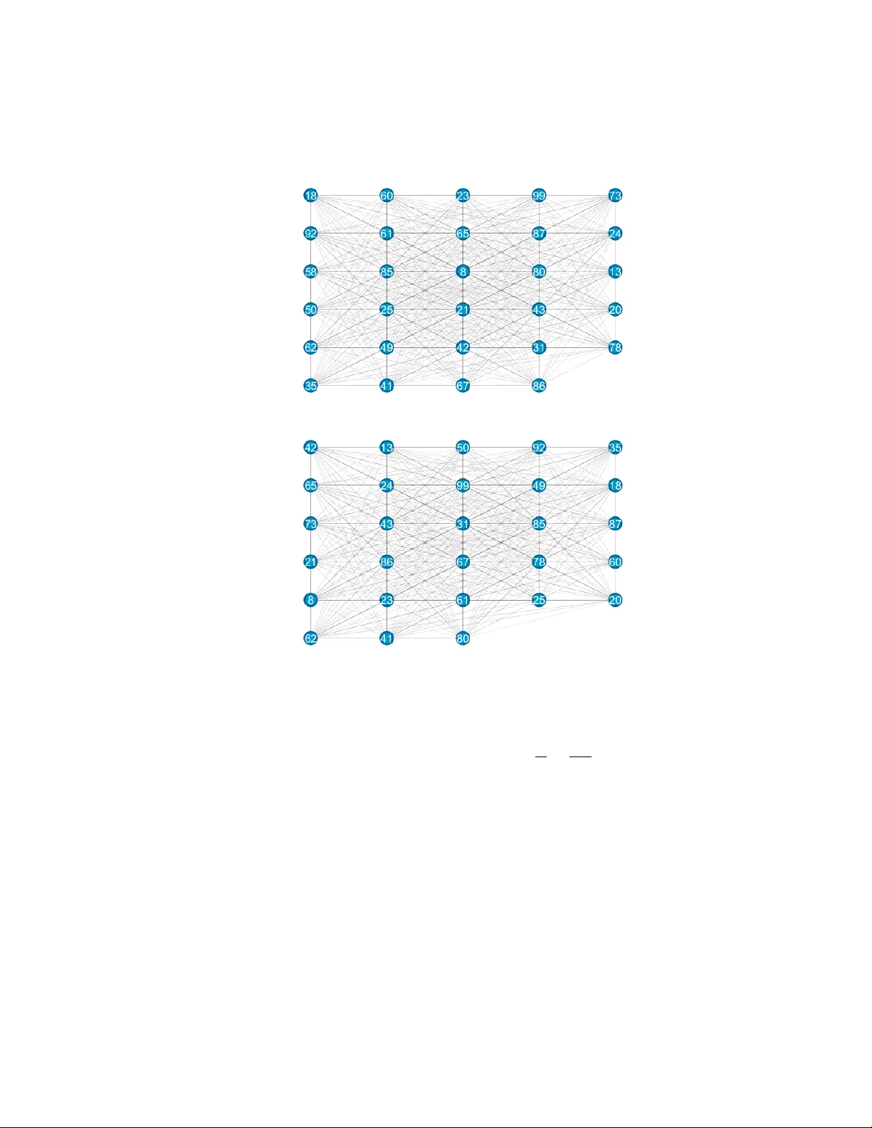
Exact Hybrid Cov ariance Thr esholding f or J oint Graphical Lasso Qingming T ang † Chao Y ang † Jian Peng ‡ Jinbo Xu † † T oyota T echnological Institute at Chicago { qmtang,harryyang,j3xu } @ttic.edu ‡ Univ ersity of Illinois at Urbana-Champaign jianpeng@illinois.edu Abstract. This paper studies precision matrix estimation for multiple related Gaussian graphical models from a dataset consisting of different classes, based upon the formulation of this problem as group graphical lasso. In particular, this paper proposes a no vel hybrid cov ariance thresholding algorithm that can ef- fectiv ely identify zero entries in the precision matrices and split a large joint graphical lasso problem into many small subproblems. Our hybrid cov ariance thresholding method is superior to existing uniform thresholding methods in that our method can split the precision matrix of each individual class using differ - ent partition schemes and thus, split group graphical lasso into much smaller subproblems, each of which can be solved very fast. This paper also establishes necessary and sufficient conditions for our hybrid cov ariance thresholding algo- rithm. Experimental results on both synthetic and real data validate the superior performance of our thresholding method ov er the others. 1 Introduction Graphs hav e been widely used to describe the relationship between variables (or fea- tures). Estimating an undirected graphical model from a dataset has been extensi vely studied. When the dataset has a Gaussian distribution, the problem is equiv alent to es- timating a precision matrix from the empirical (or sample) cov ariance matrix. In many real-world applications, the precision matrix is sparse. This problem can be formulated as graphical lasso [1, 22] and many algorithms [4, 16, 9, 19, 18] hav e been proposed to solve it. T o take advantage of the sparsity of the precision matrix, some cov ariance thresholding (also called screening) methods are de veloped to detect zero entries in the matrix and then split the matrix into smaller submatrices, which can significantly speed up the process of estimating the entire precision matrix [19, 12]. Recently , there are a fe w studies on ho w to jointly estimate multiple related graphi- cal models from a dataset with a few distinct class labels [3, 6, 7, 8, 11, 13, 14, 24, 25, 20, 23]. The underlying reason for joint estimation is that the graphs of these classes are similar to some degree, so it can increase statistical power and estimation accuracy by aggregating data of different classes. This joint graph estimation problem can be for- mulated as joint graphical lasso that makes use of similarity of the underlying graphs. In addition to group graphical lasso, Guo et al. used a non-conv e x hierarchical penalty to promote similar patterns among multiple graphical models [6] ; [3] introduced popu- lar group and fused graphical lasso; and [25, 20] proposed efficient algorithms to solve fused graphical lasso. T o model gene networks, [14] proposed a node-based penalty to promote hub structure in a graph. Existing algorithms for solving joint graphical lasso do not scale well with respect to the number of classes, denoted as K , and the number of variables, denoted as p . Similar to cov ariance thresholding methods for graphical lasso, a couple of threshold- ing methods [25, 20] are dev eloped to split a large joint graphical lasso problem into subproblems [3]. Ne v ertheless, these algorithms all use uniform thresholding to decom- pose the precision matrices of distinct classes in exactly the same way . As such, it may not split the precision matrices into small enough submatrices especially when there are a large number of classes and/or the precision matrices ha v e dif ferent sparsity patterns. Therefore, the speedup effect of co v ariance thresholding may not be very significant. In contrast to the abov e-mentioned uniform cov ariance thresholding, this paper presents a nov el hybrid (or non-uniform) thresholding approach that can divide the precision matrix for each individual class into smaller submatrices without requiring that the resultant partition schemes be exactly the same across all the classes. Using this method, we can split a large joint graphical lasso problem into much smaller sub- problems. Then we employ the popular ADMM (Alternating Direction Method of Mul- tipliers [2, 5]) method to solve joint graphical lasso based upon this hybrid partition scheme. Experiments sho w that our method can solve group graphical lasso much more efficiently than uniform thresholding. This hybrid thresholding approach is deri ved based upon group graphical lasso. The idea can also be generalized to other joint graphical lasso such as fused graphical lasso. Due to space limit, the proofs of some of the theorems in the paper are presented in supplementary material. 2 Notation and Definition In this paper , we use a script letter, like H , to denote a set or a set partition. When H is a set, we use H i to denote the i th element. Similarly we use a bold letter , like H to denote a graph, a vector or a matrix. When H is a matrix we use H i,j to denote its ( i, j ) th entry . W e use {H (1) , H (2) , . . . , H ( N ) } and { H (1) , H (2) . . . , H ( N ) } to denote N objects of same category . Let { X (1) , X (2) , . . . , X ( K ) } denote a sample dataset of K classes and the data in X ( k ) (1 ≤ k ≤ K ) are independently and identically drawn from a p -dimension normal distrib ution N ( µ ( k ) , Σ ( k ) ) . Let S ( k ) and ˆ Θ ( k ) denote the empirical covariance and (optimal) precision matrices of class k , respectively . By “optimal” we mean the precision matrices are obtained by exactly solving joint graphical lasso. Let a binary matrix E ( k ) denote the sparsity pattern of ˆ Θ ( k ) , i.e., for any i, j (1 ≤ i, j ≤ p ) , E ( k ) i,j = 1 if and only if ˆ Θ ( k ) i,j 6 = 0 . Set partition. A set H is a partition of a set C when the following conditions are satisfied: 1) any element in H is a subset of C ; 2) the union of all the elements in H is equal to C ; and 3) any tw o elements in H are disjoint. Gi v en two partitions H and F of a set C , we say that H is finer than F (or H is a refinement of F ), denoted as H  F , if ev ery element in H is a subset of some element in F . If H  F and H 6 = F , we say that H is strictly finer than F (or H is a strict refinement of F ), denoted as H ≺ F . Let Θ denote a matrix describing the pairwise relationship of elements in a set C , where Θ i,j corresponds to two elements C i and C j . Gi ven a partition H of C , we define Θ H k as a |H k | × |H k | submatrix of Θ where H k is an element of H and ( Θ H k ) i,j ∼ = Θ ( H k ) i ( H k ) j for any suitable ( i, j ). Graph-based partition. Let V = { 1 , 2 , . . . , p } denote the variable (or feature) set of the dataset. Let graph G ( k ) = ( V , E ( k ) ) denote the k th estimated concentration graph 1 ≤ k ≤ K . This graph defines a partition  ( k ) of V , where an element in  ( k ) corresponds to a connected component in G ( k ) . The matrix ˆ Θ ( k ) can be divided into disjoint submatrices based upon  ( k ) . Let E denote the mix of E (1) , E (2) , . . . , E ( K ) , i.e., one entry E i,j is equal to 1 if there exists at least one k (1 ≤ k ≤ K ) such that E ( k ) i,j is equal to 1. W e can construct a partition  of V from graph G = {V , E } , where an element in  corresponds to a connected component in G . Obviously ,  ( k ) 4  holds since E ( k ) is a subset of E . This implies that for any k , the matrix ˆ Θ ( k ) can be divided into disjoint submatrices based upon  . Feasible partition. A partition H of V is feasible for class k or graph G ( k ) if  ( k ) 4 H . This implies that 1) H can be obtained by merging some elements in  ( k ) ; 2) each element in H corresponds to a union of some connected components in graph G ( k ) ; and 3) we can divide the precision matrix ˆ Θ ( k ) into independent submatrices according to H and then separately estimate the submatrices without losing accuracy . H is uniformly feasible if for all k (1 ≤ k ≤ K ) ,  ( k ) 4 H holds. Let H (1) , H (2) , . . . , H ( K ) denote K partitions of the variable set V . If for each k (1 ≤ k ≤ K ) ,  ( k ) 4 H ( k ) holds, we say {H (1) , H (2) , . . . , H ( K ) } is a feasi- ble partition of V for the K classes or graphs. When at least two of the K partitions are not same, we say {H (1) , H (2) , . . . , H ( K ) } is a non-uniform partition. Otherwise, {H (1) , H (2) , . . . , H ( K ) } is a class-independent or uniform partition and abbreviated as H . That is, H is uniformly feasible if for all k (1 ≤ k ≤ K ) ,  ( k ) 4 H holds. Ob- viously , {  (1) ,  (2) , . . . ,  ( K ) } is finer than any non-uniform feasible partition of the K classes. Based upon the above definitions, we hav e the following theorem, which is prov ed in supplementary material. Theorem 1 F or any uniformly feasible partition H of the variable set V , we have  4 H . That is, H is feasible for graph G and  is the finest uniform feasible partition. Pr oof . First, for any element H j in H , G does not contain edges between H j and H − H j . Otherwise, since G is the mixing (or union) of all G ( k ) , there exists at least one graph G ( k ) such that it contains at least one edge between H j and H − H j . Since H j is the union of some elements in  ( k ) , this implies that there exist two different elements in  ( k ) such that G ( k ) contains edges between them, which contradicts with the fact that G ( k ) does not contain edges between any two elements in  ( k ) . That is, H is feasible for graph G . Second, if  4 H does not hold, then there is one element  i in  and one element H j in H such that  i ∩ H j 6 = ∅ and  i − H j 6 = ∅ . Based on the above paragraph, ∀ x ∈  i ∩ H j and ∀ y ∈  i − H j =  i ∩ ( H i − H j ) , we ha v e E x,y = E y ,x = 0 . That is,  i can be split into at least two disjoint subsets such that G does not contain any edges between them. This contradicts with the fact that  i corresponds to a connected component in graph G . 3 Joint Graphical Lasso T o learn the underlying graph structure of multiple classes simultaneously , some penalty functions are used to promote similar structural patterns among different classes, includ- ing [16, 3, 6, 7, 13, 14, 25, 20, 21]. A typical joint graphical lasso is formulated as the following optimization problem: min K X k =1 L ( Θ ( k ) ) + P ( Θ ) (1) Where Θ ( k )  0 is the precision matrix ( k = 1 , . . . , K ) and Θ represents the set of Θ ( k ) . The negati v e log-likelihood L ( Θ ( k ) ) and the regularization P ( Θ ) are defined as follows. L ( Θ ( k ) ) = − log det( Θ ( k ) ) + tr( S ( k ) Θ ( k ) ) (2) P ( Θ ) = λ 1 K X k =1 k Θ ( k ) k 1 + λ 2 J ( Θ ) (3) Here λ 1 > 0 and λ 2 > 0 and J ( Θ ) is some penalty function used to encourage similarity (of the structural patterns) among the K classes. In this paper, we focus on group graphical lasso. That is, J ( Θ ) = 2 X 1 ≤ i λ 1 and ∃ s , s.t. I ( s ) i,j = 1 if ∃ ( x, i, j ) satisfies the condition above then merge the tw o components of G ( x ) that containing variable i and j into new component; for ∀ ( m, n ) in this new component do Set I ( x ) m,n = I ( x ) n,m = 1 ; end for end if until No such kind of triple. retur n the connected components of each graph which define the non-uniform feasible solu- tion Algorithm 1 is a covariance thresholding algorithm that can identify a non-uniform feasible partition satisfying condition (8). W e call Algorithm 1 hybrid screening al- gorithm as it utilizes both class-specific thresholding (e.g. | S ( k ) i,j | ≤ λ 1 ) and global thresholding (e.g. P K k =1 ( | S ( k ) i,j | − λ 1 ) 2 + ≤ λ 2 2 ) to identify a non-uniform partition. This hybrid screening algorithm can terminate rapidly on a typical Linux machine, tested on the synthetic data described in section 7 with K = 10 and p = 10000 . W e can generate a uniform feasible partition using only the global thresholding and generate a non-uniform feasible partition by using only the class-specific thresh- olding, but such a partition is not as good as using the hybrid thresholding algorithm. Let {H (1) , H (2) , . . . , H ( K ) } , {L (1) , L (2) , . . . , L ( K ) } and G denote the partitions gen- erated by hybrid, class-specific and global thresholding algorithms, respectiv ely . It is obvious that H ( k ) 4 L ( k ) and H ( k ) 4 G for k = 1 , 2 , . . . , K since condition (8) is a combination of both global thresholding and class-specific thresholding. Figure 3 shows a toy example comparing the three screening methods using a dataset of two classes and three variables. In this example, the class-specific or the global thresholding alone cannot divide the variable set into disjoint groups, but their combination can do so. W e ha ve the follo wing theorem re garding our hybrid thresholding algorithm, which will be prov ed in Supplemental File. Fig. 3. Comparison of three thresholding strategies. The dataset contains 2 slightly different classes and 3 variables. The two sample cov ariance matrices are shown on the top of the fig- ure. The parameters used are λ 1 = 0 . 04 and λ 2 = 0 . 02 . Theorem 4 The hybrid scr eening algorithm yields the finest non-uniform feasible par- tition satisfying condition (8). 6 Hybrid ADMM (HADMM) In this section, we describe how to apply ADMM (Alternating Direction Method of Multipliers [2, 5]) to solve joint graphical lasso based upon a non-uniform feasible partition of the variable set. According to [3], solving Eq.(1) by ADMM is equiv alent to minimizing the following scaled augmented Lagrangian form: K X k =1 L ( Θ ( k ) ) + ρ 2 K X k =1 k Θ ( k ) − Y ( k ) + U ( k ) k 2 F + P ( Y ) (9) where Y = { Y (1) , Y (1) , . . . , Y ( K ) } and U = { U (1) , U (1) , . . . , U ( K ) } are dual vari- ables. W e use the ADMM algorithm to solv e Eq.(9) iterati vely , which updates the three variables Θ , Y and U alternativ ely . The most computational-insensitiv e step is to up- date Θ given Y and U , which requires eigen-decomposition of K matrices. W e can do this based upon a non-uniform feasible partition {H (1) , H (2) , . . . , H ( K ) } . For each k , updating Θ ( k ) giv en Y ( k ) and U ( k ) for Eq (9) is equiv alent to solving in total |H ( k ) | independent sub-problems. For each H ( k ) j ∈ H ( k ) , its independent sub-problem solves the following equation: ( Θ ( k ) H ( k ) j ) − 1 = S ( k ) H ( k ) j + ρ × ( Θ ( k ) H ( k ) j − Y ( k ) H ( k ) j + U ( k ) H ( k ) j ) (10) 0 20 40 60 80 100 120 140 160 180 200 −4000 −3000 −2000 −1000 0 1000 2000 Number of Iterations Objectiv Function Value HADMM ADMM Fig. 4. The objectiv e function value with respect to the number of iterations on a six classes type C data with p = 1000 , λ 1 = 0 . 0082 and λ 2 = 0 . 0015 . Solving Eq.(10) requires eigen-decomposition of small submatrices, which shall be much faster than the eigen-decomposition of the original large matrices. Based upon our non-uniform partition, updating Y giv en Θ and U and updating U giv en Y and Θ are also faster than the corresponding components of the plain ADMM algorithm described in [3], since our non-uniform thresholding algorithm can detect many more zero entries before ADMM is applied. 7 Experimental Results W e tested our method, denoted as HADMM (i.e., hybrid cov ariance thresholding al- gorithm + ADMM), on both synthetic and real data and compared HADMM with two control methods: 1) GADMM: global covariance thresholding algorithm + ADMM; and 2) LADMM: class-specific covariance thresholding algorithm +ADMM. W e im- plemented these methods with C++ and R, and tested them on a Linux machine with Intel Xeon E5-2670 2.6GHz. T o generate a dataset with K classes from Gaussian distribution, we first randomly generate K precision matrices and then use them to sample 5 × p data points for each class. T o make sure that the randomly-generated precision matrices are positi ve definite, we set all the diagonal entries to 5.0, and an of f-diagonal entry to either 0 or ± r × 5 . 0 . W e generate three types of datasets as follows. – T ype A : 97% of the entries in a precision matrix are 0. 2 3 4 5 6 7 8 9 10 4 5 6 7 8 9 10 11 Number of Classes Logarithm of Time(s) HADMM GADMM LADMM 2 3 4 5 6 7 8 9 10 3 4 5 6 7 8 9 10 11 12 Number of Classes Logarithm of Time(s) HADMM GADMM LADMM 2 3 4 5 6 7 8 9 10 5 6 7 8 9 10 11 12 13 Number of Classes Logarithm of Time(s) HADMM GADMM LADMM (a) T ype A 2 3 4 5 6 7 8 9 10 4 5 6 7 8 9 10 11 Number of Classes Logarithm of Time(s) HADMM GADMM LADMM 2 3 4 5 6 7 8 9 10 5 6 7 8 9 10 11 12 Number of Classes Logarithm of Time(s) HADMM GADMM LADMM 2 3 4 5 6 7 8 9 10 4 5 6 7 8 9 10 11 Number of Classes Logarithm of Time(s) HADMM GADMM LADMM (b) T ype B 2 3 4 5 6 7 8 9 10 5 6 7 8 9 10 11 12 13 Number of Classes Logarithm of Time(s) HADMM GADMM LADMM 2 3 4 5 6 7 8 9 10 5 6 7 8 9 10 11 Number of Classes Logarithm of Time(s) HADMM GADMM LADMM 2 3 4 5 6 7 8 9 10 6 6.5 7 7.5 8 8.5 9 9.5 10 10.5 11 Number of Classes Logarithm of Time(s) HADMM GADMM LADMM (c) T ype C Fig. 5. Logarithm of the running time (in seconds) of HADMM, LADMM and GADMM for p = 1000 on T ype A, T ype B and T ype C data. – T ype B : the K precision matrices have same diagonal block structure. – T ype C : the K precision matrices ha ve slightly dif ferent diagonal block structures. For T ype A , r is set to be less than 0.0061. For T ype B and T ype C , r is smaller than 0.0067. For each type we generate 18 datasets by setting K = 2 , 3 , . . . , 10 , and p = 1000 , 10000 , respecti vely . 7.1 Corr ectness of HADMM by Experimental V alidation W e first show that HADMM can conv erge to the same solution obtained by the plain ADMM (i.e., ADMM without any co variance thresholding) through experiments. T o e valuate the correctness of our method HADMM, we compare the objectiv e function value generated by HADMM to that by ADMM with respect to the number of iterations. W e run the two methods for 500 iterations over the three types of data with p = 1000 . As shown in T able 1, in the first 4 iterations, HADMM and ADMM T able 1. Objective function values of HADMM and ADMM on the six classes type C data (first 4 iterations, p = 1000 , λ 1 = 0 . 0082 , λ 2 = 0 . 0015 ) Iteration 1 2 3 4 ADMM 1713.66 -283.743 -1191.94 -1722.53 HADMM 1734.42 -265.073 -1183.73 -1719.78 yield slightly different objectiv e function values. Howe ver , along with more iterations passed, both HADMM and ADMM con verge to the same objective function v alue, as shown in Figure 4 and Supplementary Figures S3-5. This experimental result confirms that our hybrid cov ariance thresholding algorithm is correct. W e tested sev eral pairs of hyper-parameters ( λ 1 and λ 2 ) in our experiment. Please refer to the supplementary material for model selection. Note that although in terms of the number of iterations HADMM and ADMM conv erge similarly , HADMM runs much faster than ADMM at each iteration, so HADMM con verges in a much shorter time. 7.2 P erformance on Synthetic Data In pre vious section we ha ve sho wn that our HADMM con verges to the same solution as ADMM. Here we test the running times of HADMM, LADMM and GADMM needed to reach the following stop criteria for p = 1000 : P k i =1 || Θ ( k ) − Y ( k ) || < 10 − 6 and P k i =1 || Y ( k +1) − Y ( k ) || < 10 − 6 . For p = 10000 , considering the large amount of running time needed for LADMM and GADMM, we run only 50 iterations for all the three methods and then compare the av erage running time for a single iteration. W e tested the running time of the three methods using different parameters λ 1 and λ 2 ov er the three types of data. See supplementary material for model selection. W e show the result for p = 1000 in Figure 5 and that for p = 10000 in Figure S15-23 in supplementary material, respectiv ely . In Figure 5, each row shows the experimental results on one type of data ( T ype A , T ype B and T ype C from top to bottom). Each column has the experimental re- sults for the same hyper-parameters ( λ 1 = 0 . 009 and λ 2 = 0 . 0005 , λ 1 = 0 . 0086 and λ 2 = 0 . 001 , and λ 1 = 0 . 0082 and λ 2 = 0 . 0015 from left to right). As shown in Figure 5, HADMM is much more efficient than LADMM and GADMM. GADMM performs comparably to or better than LADMM when λ 2 is large. The running time of LADMM increases as λ 1 decreases. Also, the running time of all the three methods increases along with the number of classes. Howe ver , GADMM is more sensitive to the number of classes than our HADMM. Moreo ver , as our h ybrid co variance thresholding algorithm yields finer non-uniform feasible partitions, the precision matrices are more likely to be split into man y more smaller submatrices. This means it is potentially easier to parallelize HADMM to obtain ev en more speedup. W e also compare the three screening algorithms in terms of the estimated compu- tational comple xity for matrix eigen-decomposition, a time-consuming subroutine used by the ADMM algorithms. Given a partition H of the variable set of V , the compu- tational complexity can be estimated by P H i ∈H |H i | 3 . As shown in Supplementary Fig. 6. Network of the first 100 genes of class one and class three for Setting 1 . Figures S6-14, when p = 1000 , our non-uniform thresholding algorithm generates par- titions with much smaller computational complexity , usually 1 10 ∼ 1 1000 of the other two methods. Note that in these figures the Y -axis is the logarithm of the estimated compu- tational complexity . When p = 10000 , the advantage of our non-uniform thresholding algorithm ov er the other two are even larger , as shown in Figure S24-32 in Supplemental File. 7.3 P erformance on Real Gene Expr ession Data W e test our proposed method on real gene expression data. W e use a lung cancer data (accession number GDS2771 [17]) downloaded from Gene Expression Omnibus and a mouse immune dataset described in [10]. The immune dataset consists of 214 ob- servations. The lung cancer data is collected from 97 patients with lung cancer and 90 controls without lung cancer, so this lung cancer dataset consists of two different classes: patient and control. W e treat the 214 observations from the immune dataset, the 97 lung cancer observations and the 90 controls as three classes of a compound dataset for our joint inference task. These three classes share 10726 common genes, so this dataset has 10726 features and 3 classes. As the absolute value of entries of cov ariance matrix of first class (corresponds to immune observ ations) are relativ ely larger , so we divide each entry of this cov ariance matrix by 2 to make the three covariance matrices with similar magnitude before performing joint analysis using unique λ 1 and λ 2 . The running time (first 10 iterations) of HADMM, LADMM and GADMM for this compound dataset under different settings are shown in T able 2 and the resultant gene networks with dif ferent sparsity are shown in Fig 6 and Supplemental File. As shown in T able 2, HADMM (ADMM + our hybrid screening algorithm) is al- ways more ef ficient than the other tw o methods in different settings. T ypically , when λ 1 is small and λ 2 is large ( Setting 1 ), our method is much faster than LADMM. In con- trast, when λ 2 is small and λ 1 is large enough ( Setting 4 and Setting 5 ), our method is much faster than GADMM. What’ s more, when both λ 1 and λ 2 are with moderate values ( Setting 2 and Setting 3 ), HADMM is still much faster than both GADMM and LADMM. T able 2. Running time (hours) of HADMM, LADMM and GADMM on real data. ( Setting 1 : λ 1 = 0 . 1 and λ 2 = 0 . 5 ; Setting 2 : λ 1 = 0 . 2 and λ 2 = 0 . 2 ; Setting 3 : λ 1 = 0 . 3 and λ 2 = 0 . 1 ; Setting 4 : λ 1 = 0 . 4 and λ 2 = 0 . 05 , and Setting 5 : λ 1 = 0 . 5 and λ 2 = 0 . 01 ) Method Setting 1 Setting 2 Setting 3 Setting 4 Setting 5 HADMM 3.46 8.23 3.9 1.71 1.11 LADMM > 20 > 20 13.6 3.72 1.98 GADMM 4.2 > 20 > 20 11.04 6.93 As sho wn in Fig 6, the two resultant netw orks are with very similar topology struc- ture. This is reasonable because we use large λ 2 in Setting 1 . Actually , the networks of all the three classes under Setting 1 share very similar topology structure. What’ s more, the number of edges in the network does decrease significantly as λ 1 goes to 0 . 5 , as shown in Supplementary material. 8 Conclusion and Discussion This paper has presented a non-uniform or hybrid covariance thresholding algorithm to speed up solving group graphical lasso. W e have established necessary and sufficient conditions for this thresholding algorithm. Theoretical analysis and experimental tests demonstrate the effecti veness of our algorithm. Although this paper focuses only on group graphical lasso, the proposed ideas and techniques may also be e xtended to fused graphical lasso. In the paper , we simply show how to combine our covariance thresholding algo- rithm with ADMM to solve group graphical lasso. In fact, our thresholding algorithm can be combined with other methods dev eloped for (joint) graphical lasso such as the QUIC algorithm [9], the proximal gradient method [16], and even the quadratic method dev eloped for fused graphical lasso [20]. The thresholding algorithm presented in this paper is static in the sense that it is applied as a pre-processing step before ADMM is applied to solve group graphical lasso. W e can extend this “static” thresholding algorithm to a “dynamic” version. For example, we can identify zero entries in the precision matrix of a specific class based upon intermediate estimation of the precision matrices of the other classes. By doing so, we shall be able to obtain finer feasible partitions and further improve the computational efficienc y . Bibliography [1] Banerjee, O., El Ghaoui, L., d’Aspremont, A.: Model selection through sparse maximum likelihood estimation for multiv ariate gaussian or binary data. The Jour - nal of Machine Learning Research 9, 485–516 (2008) [2] Boyd, S., Parikh, N., Chu, E., Peleato, B., Eckstein, J.: Distributed optimization and statistical learning via the alternating direction method of multipliers. Foun- dations and T rends R  in Machine Learning 3(1), 1–122 (2011) [3] Danaher , P ., W ang, P ., Witten, D.M.: The joint graphical lasso for in verse covari- ance estimation across multiple classes. Journal of the Royal Statistical Society: Series B (Statistical Methodology) 76(2), 373–397 (2014) [4] Friedman, J., Hastie, T ., T ibshirani, R.: Sparse in verse cov ariance estimation with the graphical lasso. Biostatistics 9(3), 432–441 (2008) [5] Gabay , D., Mercier, B.: A dual algorithm for the solution of nonlinear variational problems via finite element approximation. Computers & Mathematics with Ap- plications 2(1), 17–40 (1976) [6] Guo, J., Levina, E., Michailidis, G., Zhu, J.: Joint estimation of multiple graphical models. Biometrika p. asq060 (2011) [7] Hara, S., W ashio, T .: Common substructure learning of multiple graphical gaus- sian models. In: Machine learning and knowledge discovery in databases, pp. 1– 16. Springer (2011) [8] Honorio, J., Samaras, D.: Multi-task learning of gaussian graphical models. In: Proceedings of the 27th International Conference on Machine Learning (ICML- 10). pp. 447–454 (2010) [9] Hsieh, C.J., Dhillon, I.S., Ravikumar , P .K., Sustik, M.A.: Sparse inv erse cov ari- ance matrix estimation using quadratic approximation. In: Advances in Neural Information Processing Systems. pp. 2330–2338 (2011) [10] Jojic, V ., Shay , T ., Sylvia, K., Zuk, O., Sun, X., Kang, J., Rege v , A., K oller, D., Consortium, I.G.P ., et al.: Identification of transcriptional regulators in the mouse immune system. Nature immunology 14(6), 633–643 (2013) [11] Liu, J., Y uan, L., Y e, J.: An ef ficient algorithm for a class of fused lasso problems. In: Proceedings of the 16th A CM SIGKDD international conference on Knowl- edge discov ery and data mining. pp. 323–332. ACM (2010) [12] Mazumder , R., Hastie, T .: Exact cov ariance thresholding into connected compo- nents for large-scale graphical lasso. The Journal of Machine Learning Research 13(1), 781–794 (2012) [13] Mohan, K., Chung, M., Han, S., W itten, D., Lee, S.I., F azel, M.: Structured learn- ing of gaussian graphical models. In: Adv ances in neural information processing systems. pp. 620–628 (2012) [14] Mohan, K., London, P ., Fazel, M., Witten, D., Lee, S.I.: Node-based learning of multiple gaussian graphical models. The Journal of Machine Learning Research 15(1), 445–488 (2014) [15] Oztoprak, F ., Nocedal, J., Rennie, S., Olsen, P .A.: Ne wton-like methods for sparse in verse covariance estimation. In: Advances in Neural Information Processing Systems. pp. 755–763 (2012) [16] Rolfs, B., Rajaratnam, B., Guillot, D., W ong, I., Maleki, A.: Iterative threshold- ing algorithm for sparse in verse cov ariance estimation. In: Advances in Neural Information Processing Systems. pp. 1574–1582 (2012) [17] Spira, A., Beane, J.E., Shah, V ., Steiling, K., Liu, G., Schembri, F ., Gilman, S., Dumas, Y .M., Calner , P ., Sebastiani, P ., et al.: Airway epithelial gene expression in the diagnostic ev aluation of smokers with suspect lung cancer . Nature medicine 13(3), 361–366 (2007) [18] Tseng, P ., Y un, S.: Block-coordinate gradient descent method for linearly con- strained nonsmooth separable optimization. Journal of Optimization Theory and Applications 140(3), 513–535 (2009) [19] W itten, D.M., Friedman, J.H., Simon, N.: New insights and faster computations for the graphical lasso. Journal of Computational and Graphical Statistics 20(4), 892–900 (2011) [20] Y ang, S., Lu, Z., Shen, X., W onka, P ., Y e, J.: Fused multiple graphical lasso. arXiv preprint arXiv:1209.2139 (2012) [21] Y uan, M., Lin, Y .: Model selection and estimation in regression with grouped v ari- ables. Journal of the Royal Statistical Society: Series B (Statistical Methodology) 68(1), 49–67 (2006) [22] Y uan, M., Lin, Y .: Model selection and estimation in the g aussian graphical model. Biometrika 94(1), 19–35 (2007) [23] Y uan, X.: Alternating direction method for covariance selection models. Journal of Scientific Computing 51(2), 261–273 (2012) [24] Zhou, S., Lafferty , J., W asserman, L.: T ime varying undirected graphs. Machine Learning 80(2-3), 295–319 (2010) [25] Zhu, Y ., Shen, X., Pan, W .: Structural pursuit over multiple undirected graphs. Journal of the American Statistical Association 109(508), 1683–1696 (2014)