Complexity penalized hydraulic fracture localization and moment tensor estimation under limited model information

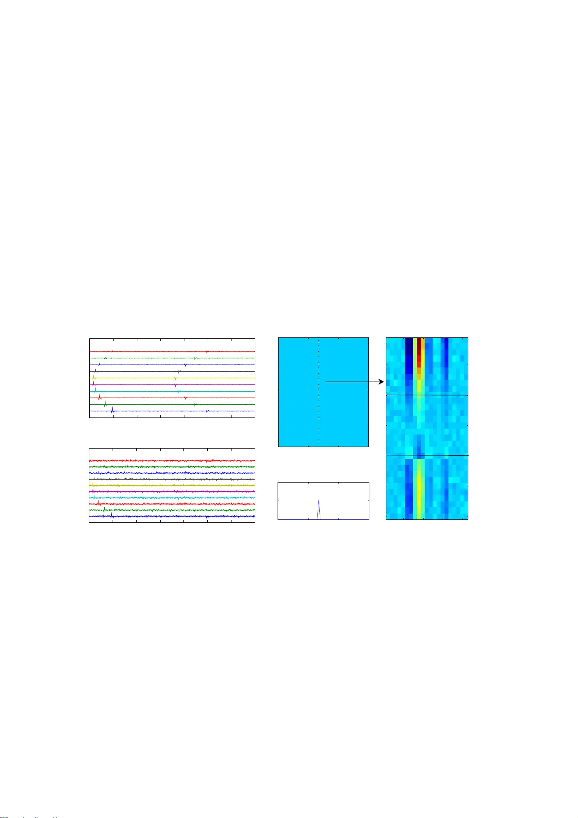
I N T R O D U C T I O N Accurate seismic hydraulic fracturing monitoring (HFM) can mitigate many of the environ- mental impacts by providing a clear real-time image of where the fractures are o ccurr ing outside of the sh ale and how effici en t l y they are formed within the gas deposit. Although simple in prin- ciple, r eal ti me monitoring of hydraul ic fracturing is extremely difficul t to p erform successfull y due to high noise levels generated by the pumpin g equipment, anisotropic propagation of seismic wa ves th rough shale , and the mul t i -la yered strati gr ap hy leading to complex seismic r a y propaga- tion, [1, 2, 3]. In addition the complexity of the source mechanism affects the relative amplitudes across the seismometers , [4] introdu c ing extra parameters in the system. Typical approaches for microseismic loc alization consists of de-noisin g of individ ual traces [5, 6] followed by time localizati on of t h e events of in t er est and then using a forward model under known strat i graphy to match the wave forms and ar rival times, [7, 8]. The pol ar ization estimation is achieved via Hodogram analysis [9] or max-likelihood type estimation [8]. I n contrast to these approaches, recently the problem of moment tensor estimation and source localization was considered in [10] for general sources and in [11] for isotropic sour ces which exploit sparsity in the n umber of mi- croseismic events in the volume to be monitored. This app r oac h i s shown to be more robust and can han d le p rocessing of multip le events at the same t ime . Although our app roach is very similar to t he approach in [10] t he main differenc e lies in the use of amplitude information from the Green’s functi on. Here we don’t use the ampli tude (of t he received wa veform) i nformation but on l y t h e tempor a l supp or t information or arrivals which is c ompletely dict ated by the velocity model of the strat i graphy and the source rec ei ver configuration. Since we are not usi ng any ampl itude information, we usually h ave more er r or in estimation an d require more rec eive rs for localiz ation. Nevertheless , when the computation of Green’s fun ction is costly or accu rate computation is not available our method can be employed. Furthermore, du e to ampli tude i n dependent processing our methods can be extended to han dle the anisotropi c cases using just t h e trave l-time i n formation for inversion, [12, 13]. M I C R O S E I S M I C S O U R C E A N D D ATA M O D E L x y z x y z θ φ source receiver e θ e φ e r search volume P P P sh P sv F I G U R E 1 : This figure shows the geome try and coord i nate system used in this pa per . In this pap er we focus on isotr opic layered media as the model for str at ig- raphy . The set-up is shown in Fig- ure 1 where a seismic event with a symmetric moment tensor M ∈ R 3 × 3 is recorded at a set of J tri -axial seis- mometers indexed as j = 1, 2, ..., J with locations r j . Let the locati on of the source/seismic e vent be denoted by l . All these locati ons are with r espect to a global co-ordinate system. The seis- mometer records compr ess ional wa ve denoted by p, and vertical and horizon- tal shear waves denoted by s v and s h respectively . Assuming ([2], [Chapter 4]) that the volume chan ges over ti me does not change the geometry of the source, the particle motion magnitude vector (say) u c ( l , j , t ) at the three axes of the seismometer j as a fun ction of time t , can then be descr i bed by the following equati on, u c ( l , j , t ) = R c ( θ , φ ) 4 π d l j ρ c 3 P l j c ψ c µ t − d l j v c ¶ (1) where d l j is th e radial distance from the source to receiver; c ∈ { p , s h , s v } is the given wave type, and ρ is the d ensity , an d R c is the rad iation pattern whi ch is a function of the moment tensor , the take off direction parameters θ j , φ j with respect to the receiver j . P l j c is the un it polarization vector for the wa ve c at the r ec eive r j . Up to a fi r st ord er approximation [14] we assume th at ψ c ( t ) ≈ ψ ( t ) for all th e wa ve types and hen c eforth will be referred t o as the source signal. Note that for isotropic formations and for compressional waves P l j p is al igned wit h the inci dence direction as determined by the ray p r opagation. The polari z ation vectors for the s h an d s v correspond to the other mutu ally per p endicular d irections . The r ad iation pattern depends on the moment tensor M and is related to th e take off dir ection at the source with r espect to the receiver j defined as the radial unit vector e r j relative to the sour ce as determined by ( θ j , φ j ), see Figure 1. Likewise we denote by unit vectors e θ j and e φ j the radial coordi nate system orthogonal to radial uni t vector . The rad iation p at t er n for a comp r essional source R p ( θ j , φ j ) is then given by , R p ( θ j , φ j ) = e T r j Me r j = £ e r j x e r j y e r j z ¤   M x x M x y M x z M x y M y y M y z M x z M y z M z z     e r j x e r j y e r j z   (2) The radiation pattern can then be simplifi ed and described as the inner produc t of the vectorized compressional unit vector product, e p j , and the vectorized moment tensor , R p ( θ j , φ j ) = e T p j z }| { h e 2 r j x 2 e r j x e r j y 2 e r j x e r j z e 2 r j y 2 e r j y e r j z e 2 r j z i m (3) where m = £ M x x , M x y , M x z , M y y , M y z , M z z ¤ T and ( · ) T denotes the transpose operation. The mea- surements r eg arding th e moment tensor at the receivers can then be t h ought of as th e mea- sure of the c orresponding radiati on energy from the source. The above expression can then be used to con str uct a vector of radiation pattern a p ∈ R J across th e J revivers, with take off an- gles of ( θ j and φ j ) correspond ing to compressional uni t vectors e p j , given by a p = E p m where E p = [ e p 1 , e p 2 , ..., e p J ] T . Similarly we h a ve a s h = E s h m and a sv = E sv m . Therefore we can write the radiation pattern across J recei v ers for the three wa ve types as the product of an augmented matrix with the vectorized moment tensor . a =   a p a s h a sv   =   E p E sh E sv   | {z } E m (4) Thus the radiation p attern across the receivers a c an then be described as the prod uct of the E matrix, whi c h i s ent i rely depen d ent on t h e location of the event and the c onfiguration of the array , and the vectorized moment tensor , w h ich i s entirely dependent on the geometry of th e fault. Under the above model for seismic source and wa ve propagation, given the n oi sy data at the tri-axial seismometers, th e problem i s to estimate the event l ocation and the associated moment tensor . In contrast to existing work, our strategy for rec ov ering th e moment tensor consists of the following. First, we estimate th e l oc ation of the source and the radiation pattern (vector) acr os s the r ec eive rs using a sparsit y penaliz ed algorithm whi ch is simil ar t o th e one used in [11] but modified to acc ount for estimation of r adiation pattern for non-isotropi c sources . F ollowin g this we estimate the sourc e signal and the radiati on pattern using a singular value d ecomposition (SVD). The estimated r adiation pat tern i s then used for the inversion for the moment t en sor using the model given by Equati on (4). F O R M U L AT I O N A S A L I N E A R I N V E R S E P R O B L E M Our methodology r ests on construc tion of a suitable representation of the data acquired at the r eceiver array under which seismic event can be compactly repr esented . This c ompac tness or sparsity in representati on is then exploited for robust estimati on of event location. W e begin by F I G U R E 2 : Left: This figure shows the blo ck spa rsity we exploit in our dictionary construction. Note that the slic e of the dictionary co efficients corresponding to the correct loca tion of the event c a n be writte n as the outer product of the source signal and the amplitude pa ttern. Right: This shows a n exam ple propagator . outlining the foll owing construction. Representation of arra y data using space time propagators - Assume that the sour ce volume is d iscretized and the locati ons l are ind ex ed by l = l 1 , l 2 , ..., l i , .., l n V where n V is th e number of discretized locations. F or a given location l = l i of the event, a fixed receiver j ∈ { 1, 2, ..., J } and w ave type c , define Γ i , j , k c = { Γ i , j , k j ′ c ( t ) } J j ′ = 1 , t ∈ T r , wi th T r being the set of recordi n g time samples at the rec ei ver array , as the collection of the wa veforms , Γ i , j , k j ′ c ( t ) = ( δ ( t − t k − τ c i j ) P i j c if j ′ = j ~ 0 if j ′ 6= j , (5) which corresponds to noi se less data at the single receiver , j , as excited by an impulsive hypothet- ical seismic event i at location l i and time t k as shown in Figure 2 right. Note that τ c i j = d l i j v c is the time delay and Γ i , j , k j ′ c ∈ R | T r |× J × 3 . F or a given event location l i we collect th ese propagators to build Γ i , k c = [ Γ i , 1 , k c (:), Γ i , 2 , k c (:), . . . , Γ i , J , k c (:)] ∈ R 3 J | T r |× J (6) where (: ) denotes the MA TLAB colon operator wh ich vectori zes the given matr ix starting with the first d imension. W ith this basic c onstruction of the temporal and polarization r espon se at the set of r eceivers for a given location l i , we construct a di ctionary of propagators across the entire physical search volume indexed from 1 to n V , time support of the signal t k ∈ T s , Φ c = h Γ 1 , 1 c , Γ 1 , 2 c , . . . , Γ i , k c , . . . , Γ n V ·| T s | c i (7) W e collect the overall di c tionary of propagators for the three wave types into a single one, Φ = £ Φ p Φ s h Φ sv ¤ (8) Clearly by construction and under assumption of superposition the data denoted as Y ∈ R | T r |× 3 × J can be wr itten as Y (:) = Φ X (:) + N where N d enotes th e additive noise assumed t o G au ssian, [5] and the coefficient vector X (:) is formed of the 3-D matrix X ∈ R 3 · J ×| T s |× n V which cap tures the event location, excitation time of th e source wav eform ψ ( t ) an d the radiation pattern ac r oss th e receivers for the three types of wa ves . Under thi s model i ng the problem is converted to estimati on of X from Y given (constructed) Φ which is a lin ear i nverse pr oblem. In pr ese nce of noise and und er the severely ill-posed nature of the problem we w i ll employ a regular i zed approach to in ve rsion. In this context we note the following regardi ng th e coefficient matrix X . 1. Under the assumption that th e number of primary seismic events per unit of t i me is small the matr ix X is sp arse along t h e thir d (location index) di mensi on, i. e . c onsists of a few non-zero fronta l slices . 2. Each non-zero front al slice (correspondin g to the location of the event) is equal to ψ a T representing the amplitude (energy) variation of the source w av eform across the receivers as a functi on of the mome nt tensor . This implies that each slice is a rank-1 matrix. This is illustrated i n Figure 2 for a single event. A L G O R I T H M F O R L O C AT I O N A N D M O M E N T T E N S O R E S T I M AT I O N W e now p resent an algorithmic workflow w h ich systematically exploits these structu ral as- pects for r eliable and robust estimation of event location and moment tensor . The algori t hmic workflow consists of three steps. Step 1 : Sparsity penalized algorithm fo r location estimation - Under th e above formula- tion, we exploit the block-sparse, i.e. simultaneously sparse structur e of X for a high resolution localizati on of the mic ro-seismic events. The algorithm corresponds to the followi ng mathemati- cal opti mi zation p r oblem also known as group sparse p enalization in the literatu re [15, 16]. ˆ X = arg min X || Y (:) − Φ X (:) || 2 + λ n V X i = 1 || X (:, :, i ) || 2 (9) where || X (:, :, i ) || 2 denotes the ℓ 2 norm of the i -th slic e , λ is a sparse tuning factor that controls the group sparseness of X , i.e. th e number of non-zero slices, versus the residual error . The min- imization operation was solved using the convex solver package TFOCS [17]. The parameter λ is chosen depending on the noise level and the an ticipated n umber of eve nts. The location estimate is then given by l ˆ i where ˆ i = arg max i || ˆ X (:, :, i ) || 2 . In the followin g we denote the correspond i ng estimate of the ˆ i -th slice X (:, :, ˆ i ) by ˆ X ˆ i . Step 2: Estimation of wa veform and radiation pattern ve ctor - Once the op t imization operation descr ibed in Equation (9) is completed, the recovered slice, ˆ X ˆ i , represents the source signal ψ ( t ) modulated by th e amplit u de pattern across the r eceivers and wa ve types , a , i.e. ˆ X ˆ i = ψ a T . In order to estimate ψ an d a we take the rank-1 SVD of ˆ X ˆ i , where th e right singular vector corresponds to the estimated source signal and the left singular vector to th e estimated radiation pattern as shown in Figure 2. Note : The low-ran k str ucture of the estimated matri x can then be used t o detect if position and velocity model of the event were correctly estimated. If th e event is estimated c or rectly then the singular values of ˆ X i should decay very rapidl y . If the decay is slow , then it is li kely that the locati on is estimated incorr ectly 1 . W e discuss some methods to d eal with incor rect loc ation estimates in Section 5. Step 3: Estimation of the moment tensor - Using the loc ation estimate l ˆ i and the knowledge of the source-recei ver array configurati on we construc t the matrix E which is a function of l ˆ i and the r ec eive r c onfiguration which is known and fixed. Then using the estimate of the radiation pattern ˆ a from Step 2 we can w r ite the simple inverse p roblem ˆ a = Em . However due to errors in estimation of a and ill-con d itioning of E due to possible bad source-receiver configur ation, one needs to again r eg ularize for inversion. F or thi s we use simple Tikhonov r eg ularizati on app r oac h where the moment tensor vector m is estimated via, ˆ m = (( E T E + λ m I ) − 1 E T ) ˆ a (10) 1 Incorrect location estimates can result from poor resol u tion in discretization of the search volume or as a re su lt of high degree of co h erence between neighboring location which are equally ca pable of explaining the data. where λ m is again tun ed using some esti mates on the uncertaint y in estimation of a and accordi ng to the amount of ill-c onditioning of E . P E R F O R M A N C E O F T H E P R O P O S E D A L G O R I T H M O N S Y N T H E T I C D ATA Simulation set-up - T o test our proposed algorithm, synthetic d at a was generated for a single vertical well in a single layer i sotropic medium with compressional velocity of 1500 m/s and shear velocity of 900 m/s. Although an isotropi c earth model is often unrealistic, we choose to use it in order to r educe t h e computati onal burden of a complex laye red stratigrap hy ray tracer . It is clear that our approach does not take advantage of the isotropic model an d can be easily extended to ani sotropic and layered media with out loss of generality . The well is l ocated at the origin with 10 sensors spac ed 100 meters apar t from a d epth of 0 to 1000 meters . F or the first experiment a seismic event was simulated at (550,550,550) meters , in moderate noise result i ng in an SNR of 46 dB , with three different moment tensors: (a) isotropic mixed with shear slip, (b) compensated l inear vector d ipole mixed with isotropic and , (c) pure sl i p . The true values of the simulated moment tensor are denoted by the blue d ots in Figure 5. A 200 by 200 by 200 meter search volume was used w i th a spaci ng of 25 meters center ed aroun d the ev ent. The min imization operation in Equation (9) was then used to determine the location of the event with the resulting localizati on by p icking the slice with t h e largest ℓ 2 norm shown in Figure 3. Location Index Inter−group Index Dictionary coefficients 340 360 380 400 100 200 300 400 500 600 340 360 380 400 0 0.2 0.4 Group Norm time index receiver index Moment & Source 5 10 15 20 5 10 15 20 25 30 500 600 700 800 900 1000 1100 1200 0 2 4 6 8 10 12 p−p = 1.0e+0 X traces receiver index 500 600 700 800 900 1000 1100 1200 0 2 4 6 8 10 12 p−p = 1.2e+0 Time (ms) p sh sv SNR 52 SNR 32 F I G U R E 3 : Left : This figure shows the simulated traces along the x-axis for two noise levels. T op Middle : This figure shows the value of the re covered dictio nary coe ffi cients . Bottom Middle : This figure shows the vector of the ℓ 2 norms of the slices of the coefficient m atrix. The largest value is ta ken as the locatio n of the event. Right : This figure shows the dictionary coefficients of the corr e sponding location (slice) reshaped as a matrix. N ote that the source signal is comm o n across the re c eivers and wave types. Radiation P attern & Moment T e nsor Recovery - A r ank 1 truncated SVD was th en used to recover the sourc e fun ction and radiation patter n, as shown i n figure 4. The estimated amplitude pattern was then inverted using a ran k 5 t runcated SVD an d Tikhonov inversion with a λ of 10 − 6 , the ideal choice of truncat ion and λ will vary as func tion of sour ce receiver geometry and noise. The si mu lation and estimation of th e moment tensor an d amp litude pattern was then repeated 20 t i mes for each of the three c ases . F or all instances the events were located at the correct location and t h e estimated moment tensors are shown in fi gure 5. Both Tikhonov and truncated SVD significan tly resulted i n nearly identical r ecove ry of the moment tensor for cases (b) & (c) and greatly improved the estimations of the non-regular i zed solution. However , for test case (a) Tikhonov , SVD , an d the non-regular i zed inverse provided p oo r estimates of the moment tensor . 0 5 10 15 20 25 30 −0.6 −0.4 −0.2 0 0.2 receiver index Magnitude Radiation Pattern 2 4 6 8 10 12 14 16 18 20 −1 −0.5 0 0.5 Time (ms) Amplitude Source and Greens Estimate (correct) Truth Estimate (incorrect) Estimate (correct) Truth Estimate (incorrect) F I G U R E 4 : T op : This figu re shows the tr ue amp l itude pa ttern and the estimated amplitude pattern. Bottom : This figure shows the true and estimated source function. F or each of the two plots the reconstruction are sh own for when the locati o n of the event was estima te d corre c tly a n d incorrectly . Mxx Mxy Mxz Myy Myz Mzz −1 −0.5 0 0.5 1 Moment Tensor Component Magnitude case A Mxx Mxy Mxz Myy Myz Mzz −1 −0.5 0 0.5 1 Moment Tensor Component Magnitude case B Mxx Mxy Mxz Myy Myz Mzz −1 −0.5 0 0.5 1 Moment Tensor Component Magnitude case C SVD Pseudo Tikhonov Truth F I G U R E 5 : This figu re shows the true moment tensor and estim a ted moment tensor using the pseudo inverse with Tikhonov regularization and truncated SVD. Without the regularization the estima tes prove wildly inaccurate for all three of the test cases. Regularization improves the estimated moment tensor in cases (b) and (c) but pro vide s mi xed results for test c ase (a). 30 35 40 45 50 55 0 5 10 15 20 25 30 35 40 45 50 SNR (dB) STD (meters) SNR vs Accuracy x y z F I G U R E 6 : This figure shows depth z , down range x , and cross range y error as a function of SNR from 30 to 50 dB. Both depth and down range estimations are m uch more robust to noise than the cross range estimate. Location Accuracy - In the second experi - ment we generated a seismic event with the mo- ment tensor (a) with at the same locati on of (550,550,500) with an increased dict i onary res- olution of 5 meters. G aussian noise was then added to the simulated tr ace for 20 noise levels with a resulting SNR of 25 to 50 and th e loc ation was estimated usin g equation 9 with a λ of 3. At each of t he noise levels the process was repeated 20 times . Figure 6 shows t h e resulting locati on accurac y (one stan dard deviation) as a fun ction of SNR. Depth z and d own ran ge x estimation proved to much more robust t o noise than cross range estimations y . The poor ac curacy across the y axes location is likely due to the fact that the estimation of the cross r ange of the event i s highly dependent on the polariz ation amplitu d es of the i ncident ray which is much more sensitive to noise than the estimate of arri val times. C O N C L U S I O N & F U T U R E W O R K In this paper we have presented comprehensive approach for HFM. The appr oac h is robust towards unc er tainties i n stratigraphy models an d is flexible to incorp or ate prior informati on at each step. F or example , i n Step 3 of the algorith mic framework one c an use prior information on m and make the inversion more robust. In th i s context we are currentl y looking to i ncorporate the distribution of eigenvalues of the matrix M [18] and exploit them in recovery of the moment tensor . Similar appr oac h can be used in r ecov ery of location estimate where prior information on location can be incorporated via a weighted p enalty term li ke so P n V i = 1 w i || X (:, :, i ) || 2 in Equation (9) where if w i is i n inverse proportion to th e likelihood of l ocation l i . Estimation of the moment t en sor pr ov ed diffic ult when the l oc ation of the event was estimated incorrect l y . Wh en th e locati on was estimated incor rectly the sl i ce c orresponding to the highest group norm c ould no longer be well ap proximated by a rank-1 outer p roduct (figur e 7). The resulting recovered rad iation pattern and source funct i on somewhat matched th e simulated data but the sour ce function w as often ti me shi fted and the radiation pattern was more noisy (figure 4). Note that instead of a two step procedure to estimate the location followed by taking the SVD of the r esulting estimates of the coefficient slices one can modify the algorithm of Equation 9 to the following. ˆ X = argmin X || Y (:) − Φ X (:) || 2 + λ n V X i = 1 || X (:, :, i ) || ∗ (11) where || X (:, :, i ) || ∗ represents the nu clear norm of the i -th slice. In addi tion to implementing thi s proposed norm, we plan to valid ate our r esults using a more complex ray tracer on a anisotropic layered model. Correction Location time index receiver index 5 10 15 20 5 10 15 20 25 30 Incorrect Location time index receiver index 5 10 15 20 5 10 15 20 25 30 0 2 4 6 8 10 0 0.1 0.2 0.3 0.4 0.5 0.6 0.7 0.8 0.9 1 Eigenvalue Index Magnitude Eigenvalue Decay Correct Incorrect F I G U R E 7 : Left : This shows the unwrapped dictionary slice for a seismic event when its loca tion was estimated correctly . Middle : The unwrapped slice for an incorrectly lo cated event. Note that for the incorrect event the pattern of the source signal across the r eceivers is less constant and thus higher rank. Ri ght : this figure shows the normalized eigenvalues for the two matrices . F or the correctly estima ted ma tr ix the eigenvalues decay rapidly . R E F E R E N C E S [1] L. Eisner and P . M. Duncan , “Uncer t ai nties in passive seismic monitor ing”, The Leading Edge 28 2 8 , 648–655 (2009). [2] K. Aki and P . G. Richards , Quantitative Seismology , 2nd Edition (University Scienc e Books) (2002). [3] P . M. Shearer , Introduction to Seismology (Cambridge University Press) (2009). [4] C . H. Chapman an d W . S. Leaney , “ A new moment-tensor decomposition for seismic events in an isotropic media”, Geophysical Jo urnal International 188 , 343–370 (2012), URL http://dx.doi.org/10.1111/j.1365- 246X.2011.05265.x . [5] Q . Liu, S . Bose , H.-P . V alero, R. Shenoy , and A. Ounadjela, “Detecting small amplit u de signal and transit ti mes in h i gh noise: Appl ication to hydraul ic fracture monitoring”, in IEEE Geoscienc e and Remote Sensing Symposium (2009). [6] I. V era Rodr iguez, D . Bonar , and M. Sacchi, “Microseismic data denoi si ng u sing a 3c group sparsity constrained ti me-f requency transform”, Geophysics 77 , V21–V29 (2012), URL http://geophysics.geoscienceworld.org/content/77/2/V21.abstract . [7] D . N . Burch, “Live hydr aulic frac ture monitorin g an d diversion”, Oi lfield Review 21 (Autumn 2009). [8] B . Khadhraoui , D. Leslie, J . D rew , and R. Jones , “Real-time detecti on and locali z ation of microseismic events”, SEG T ec hnical Program Expanded Abstr ac ts 29 , 2146–2150 (2010), URL http://link.aip.org/link/?SGA/29/21 46/1 . [9] L. Han, “Microseismic monit oring and hypocenter location”, Ph.D . thesis, Department of Geoscience, Calgary , Alberta, Canada (2010). [10] I. V . Rodriguez, M. Sacchi, an d Y . J . Gu, “Simultaneous rec ov ery of or igin time, hypocen- tre locati on and seismic moment tensor usin g spar se rep r esentation theory”, Geoph ysic al Jo urnal Internation al (2012). [11] G . El y an d S. Aeron, “Robust h ydraulic fracture monitoring (hfm) of multip le time over - lapping events u sing a generalized discrete radon transform”, in Ge oscience a nd Remote Sensing Symposium (IGAR SS ), 2012 IEEE Internationa l , 622 –625 (2012). [12] C . H. Chapman and R. G . Pratt, “Traveltime tomography in anisotropic media-i. theory”, Geophysical J ournal International 1 09 , 1–19 (1992), URL http://dx.doi.org/10.1111/j.1365- 246X.1992.tb00075.x . [13] R. G . Pratt an d C . H . Chapman, “Traveltime tomography in anisotropic me- dia—ii. applic at i on”, Geophysical Journal I nternational 109 , 20–37 (1992), URL http://dx.doi.org/10.1111/j.1365- 246X.1992.tb00076.x . [14] R. Madariaga, “Seismic source th eo ry”, in T re a tise o n Ge op hysics , edited by G . Schuber t , volume 4, 59–82 (Elsev ier) (2007), URL http://dx.doi.org/10.1016/B978- 044452748- 6.00061- 4 . [15] J . A. Tropp, A. C . Gilbert, an d M. J . Strauss, “ Algorithms for simul t an eous sp arse app r oxima- tion. part II: Convex relaxation”, Signal Processing , special issue on Sparse approximations in signal and image processing 8 6 , 572–588 (2006). [16] A. Majumdar and R. W ard, “F ast group sparse classification”, Electr ical and Computer En- gineering, Canadian J ournal of 3 4 , 136 –144 (2009). [17] S . R. Becker , E. J . Candès , and M. Grant, “T emplates for c on vex cone pr ob- lems with ap plications to sparse signal r ecove ry”, ar Xiv:1009.2065 (2010), URL http://arxiv.org/abs/1009.2065 , math ematical Programming Computation, V olume 3, Number 3, 165-218, 2011. [18] A. Baig and T . Urbancic, “Microseismic moment tensors: A path to un- derstandin g frac growth”, The Leading Edge 29 , 320–324 (2010), URL http://library.seg.org/doi/abs/10.1190/1.3353729 .