Unsupervised Post-Nonlinear Unmixing of Hyperspectral Images Using a Hamiltonian Monte Carlo Algorithm
This paper presents a nonlinear mixing model for hyperspectral image unmixing. The proposed model assumes that the pixel reflectances are post-nonlinear functions of unknown pure spectral components contaminated by an additive white Gaussian noise. T…
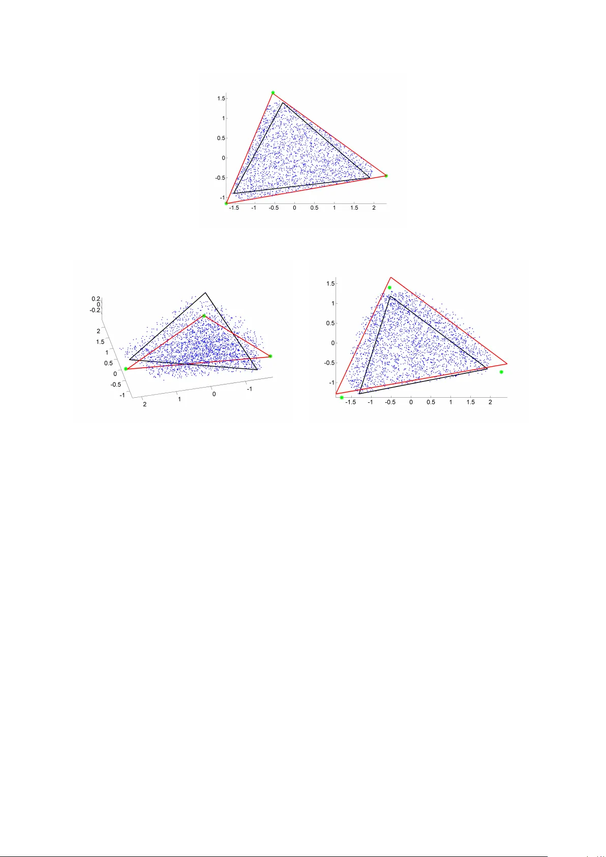
Authors: Yoann Altmann, Nicolas Dobigeon, Jean-Yves Tourneret
1 Unsupervised Post-Nonlinear Unmixing of Hyperspectral Images Using a Hamiltonian Monte Carlo Algorithm Y oann Altmann, Nicolas Dobigeon and Jean-Yves T ourneret Abstract This paper presents a nonlinear mixing model for hyperspectral image unmixing. The proposed model assumes that the pixel reflectances are post-nonlinear functions of unkno wn pure spectral components contaminated by an additi ve white Gaussian noise. These nonlinear functions are approximated using polynomials leading to a polynomial post-nonlinear mixing model. A Bayesian algorithm is proposed to estimate the parameters in volv ed in the model yielding an unsupervised nonlinear unmixing algorithm. Due to the large number of parameters to be estimated, an efficient Hamiltonian Monte Carlo algorithm is inv estigated. The classical leapfrog steps of this algorithm are modified to handle the parameter constraints. The performance of the unmixing strategy , including con ver gence and parameter tuning, is first ev aluated on synthetic data. Simulations conducted with real data finally show the accuracy of the proposed unmixing strategy for the analysis of hyperspectral images. Index T erms Hyperspectral imagery , unsupervised spectral unmixing, Hamiltonian Monte Carlo, post-nonlinear model. Part of this work has been supported by Direction Generale de l’armement, French Ministry of defence, and by the Hypanema ANR Project ANR Project n ◦ ANR- 12-BS03-003. The authors are with the University of T oulouse, IRIT/INP-ENSEEIHT/T ´ eSA, 2 rue Charles Camichel, BP 7122, 31071 T oulouse cedex 7, France (e-mail: { Y oann.Altmann, Nicolas.Dobigeon, Jean-Yves.T ourneret } @enseeiht.fr). September 28, 2018 DRAFT 2 I . I N T RO D U C T I O N Identifying macroscopic materials and quantifying the proportions of these materials are major issues when analyzing hyperspectral images. This blind source separation problem, also referred to as spectral unmixing (SU), has been widely studied for the applications where the pix el reflectances are linear combinations of pure component spectra [1]–[5]. Ho wev er , as explained in [6], [7], the linear mixing model (LMM) can be inappropriate for some hyperspectral images, such as those containing sand, trees or vegetation areas. Nonlinear mixing models (NLMMs) provide an interesting alternative for overcoming the inherent limitations of the LMM. They ha ve been proposed in the hyperspectral image literature and can be divided into two main classes. The first class of NLMMs consists of physical models based on the nature of the en vi- ronment. These models include the bidirectional reflectance based model proposed in [8] for intimate mixtures associated with sand-like materials and the bilinear models recently studied in [9]–[12] to account for scattering effects mainly observed in ve getation and urban areas. The second class of NLMMs contains more flexible models allo wing different kinds of nonlinearities to be approximated. These fle xible models are constructed from neural networks [13], [14], kernels [15], [16], or post-nonlinear transformations [17], [18]. In particular, a polynomial post-nonlinear mixing model (PPNMM) has recently shown interesting properties for the SU of hyperspectral images [19]. Most nonlinear unmixing strategies a vailable in the literature are supervised, i.e., the endmembers contained in the image are assumed to be known (chosen from a spectral library or extracted from the data by an endmember extraction algorithm (EEA)). Moreov er , most existing EEAs rely on the LMM [20]–[22] and thus can be inaccurate for nonlinear mixtures. Recently , a nonlinear EEA based on the approximation of geodesic distances has been proposed in [23] to extract endmembers from the data. Howe v er , this algorithm can suf fer from the absence of pure pixels in the image (as most linear EEAs). This paper presents a fully unsupervised Bayesian unmixing algorithm based on the PP- NMM studied in [19]. In the Bayesian frame work, appropriate prior distributions are chosen for the unknown PPNMM parameters, i.e., the endmembers, the mixing coefficients, the nonlinearity parameters and the noise variance. The joint posterior distribution of these parameters is then deri ved. Howe ver , the classical Bayesian estimators cannot be easily computed from this joint posterior . T o alleviate this problem, a Marko v chain Monte Carlo September 28, 2018 DRAFT 3 (MCMC) method is used to generate samples according to the posterior of interest. More precisely , due to the lar ge number of parameters to be estimated we propose to use a Hamiltonian Monte Carlo (HMC) [24] method to sample according to some conditional distributions associated with the posterior . HMCs are powerful simulation strategies based on Hamiltonian dynamics which can improv e the con v ergence and mixing properties of classical MCMC methods (such as the Gibbs sampler and the Metropolis-Hastings algorithm) [25], [26]. These methods have receiv ed growing interest in many applications, especially when the number of parameters to be estimated is large [27], [28]. The classical HMC can only be used for unconstrained variables. Howe v er , ne w HMC methods hav e been recently proposed to handle constrained v ariables [25, Chap. 5] [29], [30] which allow HMCs to sample according to the posterior of the Bayesian model proposed for SU. Finally , as in any MCMC method, the generated samples are used to compute Bayesian estimators as well as measures of uncertainties such as confidence interv als. The paper is or ganized as follows. Section II introduces the PPNMM for hyperspectral image analysis. Section III presents the hierarchical Bayesian model associated with the proposed PPNMM and its posterior distribution. The constrained HMC (CHMC) algorithm used to sample some parameters of this posterior is described in Section IV. The CHMC is coupled with a standard Gibbs sampler presented in Section V. Some simulation results conducted on synthetic and real data are sho wn and discussed in Sections VI and VII. Conclusions are finally reported in Section VIII. I I . P RO B L E M F O R M U L A T I O N A. P olynomial post-nonlinear mixing model This section recalls the nonlinear mixing model used in [19] for hyperspectral image SU. W e consider a set of N observed spectra y n = [ y n, 1 , . . . , y n,L ] T , n ∈ { 1 , . . . , N } where L is the number of spectral bands. Each of these spectra is defined as a nonlinear transformation g n of a linear mixture of R spectra m r contaminated by additiv e noise y n = g n R X r =1 a r,n m r ! + e n = g n ( M a n ) + e n (1) where m r = [ m r, 1 , . . . , m r,L ] T is the spectrum of the r th material present in the scene, a r,n is its corresponding proportion in the n th pix el, R is the number of endmembers contained in the image and g n is a nonlinear function associated with the n th pixel. Moreov er , e n is an additiv e independently distributed zero-mean Gaussian noise sequence with diagonal September 28, 2018 DRAFT 4 cov ariance matrix Σ = diag ( σ 2 ) , denoted as e n ∼ N ( 0 L , Σ ) , where σ 2 = [ σ 2 1 , . . . , σ 2 L ] T is the vector of the L noise variances and diag ( σ 2 ) is an L × L diagonal matrix containing the elements of the vector σ 2 . Note that the usual matrix and vector notations M = [ m 1 , . . . , m R ] and a n = [ a 1 ,n , . . . , a R,n ] T hav e been used in the right hand side of (1). As in [19], the N nonlinear functions g n are defined as second order polynomial nonlinearities defined by g n : [0 , 1] L → R L s 7→ s 1 + b n s 2 1 , . . . , s L + b n s 2 L T (2) with s = [ s 1 , . . . , s L ] T and b n is a real parameter . An interesting property of the resulting nonlinear model referred to as polynomial post nonlinear mixing model (PPNMM) is that it re- duces to the classical LMM for b n = 0 . Motiv ations for considering polynomial nonlinearities hav e been discussed in [19]. In particular , it has been shown that the PPNMM is very flexible to approximate many different nonlinearities and can be used for nonlinearity detection. Straightforward computations allo w the PPNMM observation matrix to be expressed as follo ws Y = MA + [( MA ) ( MA )] diag ( b ) + E (3) where A = [ a 1 , . . . , a N ] is an R × N matrix, Y = [ y 1 , . . . , y N ] and E = [ e 1 , . . . , e N ] are L × N matrices, b = [ b 1 , . . . , b N ] T is an N × 1 vector containing the nonlinearity parameters and denotes the Hadamard (termwise) product. B. Abundance r eparametrization Due to physical considerations, the abundance vectors a n satisfy the follo wing positivity and sum-to-one constraints R X r =1 a r,n = 1 , a r,n > 0 , ∀ r ∈ { 1 , . . . , R } . (4) T o handle these constraints, we propose to reparameterize the abundance vectors belonging to the following set S = ( a = [ a 1 , . . . , a R ] T a r > 0 , R X r =1 a r = 1 ) (5) using the following transformation a r,n = r − 1 Y k =1 z k,n ! × 1 − z r,n if r < R 1 if r = R . (6) September 28, 2018 DRAFT 5 This transformation has been recently suggested in [31]. One moti vation for using the latent v ariables z r,n instead of a r,n is the fact that the constraints (4) for the n th abundance vector a n express as 0 < z r,n < 1 , ∀ r ∈ { 1 , . . . , R − 1 } (7) for the n th coef ficient vector z n = [ z 1 ,n , . . . , z R − 1 ,n ] T . As a consequence, the constraints (7) are much easier to handle for the sampling procedure than (4) (as will be shown in Sections IV and V). The next section presents the Bayesian model associated with the PPNMM (1) for SU. I I I . B AY E S I A N M O D E L This section generalizes the hierarchical Bayesian model introduced in [19] in order to jointly estimate the abundances and endmembers, leading to a fully unsupervised hyper- spectral unmixing algorithm. The unknown parameter vector associated with the PPNMM contains the reparameterized abundances Z = [ z 1 , . . . , z N ] (satisfying the constraints (7)), the endmember matrix M , the nonlinearity parameter vector b and the additiv e noise variance σ 2 . This section summarizes the likelihood and the parameter priors (associated with the proposed hierarchical Bayesian PPNMM) introduced to perform nonlinear unsupervised hyperspectral unmixing. A. Likelihood Equation (3) shows that y n | M , z n , b n , σ 2 is distributed according to a Gaussian distribution with mean g n ( M a n ) and co variance matrix Σ , denoted as y n | M , z n , b n , σ 2 ∼ N ( g n ( M a n ) , Σ ) . Note that the abundance vector a n should be denoted as a n ( z n ) . Ho wev er , the argument z n has been omitted for brevity . Assuming independence between the observed pixels, the joint likelihood of the observ ation matrix Y can be expressed as f ( Y | M , Z , b , σ 2 ) ∝ | Σ | − N/ 2 etr − ( Y − X ) T Σ − 1 ( Y − X ) 2 (8) where ∝ means “proportional to”, etr( · ) denotes the exponential trace and X = MA + [( MA ) ( MA )] diag ( b ) is an L × N matrix. September 28, 2018 DRAFT 6 B. P arameter priors 1) Coefficient matrix Z : T o reflect the lack of prior knowledge about the abundances, we propose to assign prior distributions for the coefficient vector z n that correspond to noninformati ve prior distrib utions for a n . More precisely , assigning the following beta priors z n,r ∼ B e ( R − r , 1) r ∈ { 1 , . . . , R − 1 } (9) and assuming prior independence between the elements of z n yield an abundance vector a n uniformly distrib uted in the set defined in (5) (see [31] for details). Assuming prior independence between the coefficient vectors { z n } n =1 ,...,N leads to f ( Z ) = R − 1 Y r =1 ( 1 B ( R − r, 1) N N Y n =1 z R − r − 1 n,r ) (10) where B ( · , · ) is the Beta function. 2) Endmembers: Each endmember m r = [ m r, 1 , . . . , m r,L ] T is a reflectance vector satisfy- ing the following constraints 0 ≤ m r,` ≤ 1 , ∀ r ∈ { 1 , . . . , R } , ∀ ` ∈ { 1 , . . . , L } . (11) For each endmember m r , we propose to use a Gaussian prior m r ∼ N [0 , 1] L ( ¯ m r , s 2 I L ) , (12) truncated on [0 , 1] L to satisfy the constraints (11). In this paper , we propose to select the mean vectors ¯ m r as the pure components pre viously identified by the nonlinear EEA studied in [23] and referred to as “Heylen”. The variance s 2 reflects the degree of confidence given to this prior information. When no additional knowledge is av ailable, this variance is fixed to a lar ge v alue ( s 2 = 50 in our simulations). Note that any EEA could be used to define the vectors ¯ m 1 , . . . , ¯ m R . 3) Nonlinearity parameters: The PPNMM reduces to the LMM for b n = 0 . Since the LMM is relev ant for most observed pixels, it makes sense to assign prior distributions to the nonlinearity parameters that enforce sparsity for the vector b . T o detect linear and nonlinear mixtures of the pure spectral signatures in the image, the following conjugate Bernoulli- Gaussian prior is assigned to the nonlinearity parameter b n f ( b n | w , σ 2 b ) = (1 − w ) δ ( b n ) + w 1 p 2 π σ 2 b exp − b 2 n 2 σ 2 b (13) where δ ( · ) denotes the Dirac delta function. Note that the prior distrib utions for the non- linearity parameters { b n } n =1 ,...,N share the same hyperparameters w ∈ [0 , 1] and σ 2 b ∈ R + . September 28, 2018 DRAFT 7 More precisely , the weight w is the prior probability of ha ving a nonlinearly mixed pixel in the image. Assuming prior independence between the nonlinearity parameters { b n } n =1 ,...,N , the joint prior distribution of the nonlinearity parameter vector b can be expressed as follo ws f ( b | w, σ 2 b ) = N Y n =1 f ( b n | w , σ 2 b ) (14) 4) Noise variances: A Jeffre ys’ prior is chosen for the noise variance of each spectral band σ 2 ` f ( σ 2 ` ) ∝ 1 σ 2 ` 1 R + σ 2 ` (15) which reflects the absence of knowledge for this parameter (see [32] for motiv ations). As- suming prior independence between the noise v ariances, we obtain f ( σ 2 ) = L Y ` =1 f ( σ 2 ` ) . (16) C. Hyperparameter priors The performance of the proposed Bayesian model for spectral unmixing depends on the v alues of the hyperparameters σ 2 b and w . When the hyperparameters are difficult to adjust, it is classical to include them in the unkno wn parameter vector , resulting in a hierarchical Bayesian model [19], [33]. This strategy requires to define prior distributions for the hyperparameters. A conjugate in verse-Gamma prior is assigned to σ 2 b σ 2 b ∼ I G ( γ , ν ) (17) where ( γ , ν ) are real parameters fixed to obtain a flat prior , reflecting the absence of kno wl- edge about the v ariance σ 2 b ( ( γ , ν ) will be set to (10 − 1 , 10 − 1 ) in the simulation section). A uniform prior distribution is assigned to the hyperparameter w w ∼ U [0 , 1] ( w ) (18) since there is no a priori information regarding the proportions of linearly and nonlinearly mixed pixels in the image. The resulting directed acyclic graph (D A G) associated with the proposed Bayesian model is depicted in Fig. 1. September 28, 2018 DRAFT 8 D. Joint posterior distribution The joint posterior distribution of the unknown parameter/hyperparameter vector { θ , Φ } where θ = { Z , M , b , σ 2 } and Φ = { σ 2 b , w } can be computed using the following hierarchical structure f ( θ , Φ | Y ) ∝ f ( Y | θ , Φ ) f ( θ , Φ ) (19) where f ( Y | θ ) has been defined in (8). By assuming a priori independence between the parameters Z , M , b and σ 2 and between the hyperparameters σ b and w , the joint prior distribution of the unknown parameter vector can be expressed as f ( θ , Φ ) = f ( θ | Φ ) f ( Φ ) = f ( Z ) f ( M ) f ( σ 2 ) f ( b | σ 2 b , w ) f ( σ 2 b ) f ( w ) . (20) The joint posterior distrib ution f ( θ , Φ | Y ) can then be computed up to a multiplicati ve constant after replacing (20) and (8) in (19). Unfortunately , it is dif ficult to obtain closed form expressions for the standard Bayesian estimators (including the maximum a posteriori (MAP) and the minimum mean square error (MMSE) estimators) associated with (19). In this paper , we propose to use ef ficient Marko v Chain Monte Carlo (MCMC) methods to generate samples asymptotically distributed according to (19). Due to the large number of parameters to be sampled, we use an HMC algorithm which allo ws the number of sampling steps to be reduced and which improv es the mixing properties of the sampler . The generated samples are then used to compute the MMSE estimator of the unknown parameter vector ( θ , Φ ) . The next section summarizes the basic principles of the HMC methods that will be used to sample asymptotically from (19). I V . C O N S T R A I N E D H A M I LTO N I A N M O N T E C A R L O M E T H O D HMCs are powerful methods for sampling from many continuous distrib utions by intro- ducing fictitious momentum v ariables. Let q ∈ R D be the parameter of interest and π ( q ) its corresponding distribution to be sampled from. From statistical mechanics, the distribution π ( q ) can be related to a potential energy function U ( q ) = − log [ π ( q )] + c where c is a positi v e constant such that R exp ( − U ( q ) + c ) d q = 1 . The Hamiltonian of π ( q ) is a function of the energy U ( q ) and of an additional momentum vector p ∈ R D defined as H ( q , p ) = U ( q ) + K ( p ) (21) September 28, 2018 DRAFT 9 ν γ z z s 2 f M σ 2 b w Z ( ( M b v v σ 2 r r Y Fig. 1. D A G for the parameter and hyperparameter priors (the fixed parameters appear in boxes). where K ( p ) is an arbitrary kinetic energy function. Usually , a quadratic kinetic energy is chosen and we propose to use K ( p ) = p T p / 2 in this paper (for reasons e xplained later). The Hamiltonian (21) defines the following distribution f ( q , p ) ∝ exp [ − H ( q , p )] ∝ π ( q ) exp − 1 2 p T p (22) for ( q , p ) which shows that q and p are independent and that the marginal distribution of p is a N ( 0 D , I D ) distribution. The HMC algorithm allo ws samples to be asymptotically generated according to (22). The i th HMC iteration starts with an initial pair of vectors ( q ( i ) , p ( i ) ) and consists of two steps. The first step resamples the initial momentum ˜ p ( i ) according to the standard multi v ariate Gaussian distribution. The second step uses Hamiltonian dynamics to propose a candidate ( q ∗ , p ∗ ) which is accepted with the follo wing probability ρ = min exp − H ( q ∗ , p ∗ ) + H ( q ( i ) , ˜ p ( i ) ) , 1 . (23) A. Generation of the candidate ( q ∗ , p ∗ ) Hamiltonian dynamics are usually simulated by discretization methods such as Euler or leapfrog methods. The classical leapfrog method is a discretization scheme composed of N LF September 28, 2018 DRAFT 10 steps with a discretization stepsize . The n th leapfrog step can be expressed as p ( i,n + / 2) = p ( i,n ) − 2 ∂ U ∂ q T q ( i,n ) (24a) q ( i, ( n +1) ) = q ( i,n ) + p ( i,n + / 2) (24b) p ( i, ( n +1) ) = p ( i,n + / 2) − 2 ∂ U ∂ q T q ( i, ( n +1) ) . (24c) The leapfrog method starts with ( q ( i, 0) , ˜ p ( i ) ) = ( q ( i ) , ˜ p ( i ) ) and the candidate is set after N LF steps to ( q ∗ , p ∗ ) = ( q ( i,N LF ) , ˜ p ( i,N LF ) ) . Ho wev er , if q is subject to constraints, more sophisticated discretization methods must be used. Assume that the vector of interest q = [ q 1 , . . . , q D ] T satisfies the follo wing constraints q l < q d < q u , d ∈ { 1 , . . . , D } (25) where q l (resp. q u ) is the lower (resp. upper) bound for q d (such kind of constraints need to be satisfied by the elements of Z and the endmembers in M ). In this paper we propose to use the constrained leapfrog scheme studied in [25, Chap. 5], consisting of N LF steps, with a discretization stepsize q . Each CHMC iteration starts in a similar way to the classical leapfrog method, with the sequential sampling of the momentum p (24a) and the vector q (24b). Ho wev er , if the generated vector q violates the constraints (25), it is modified depending on the violated constraints and the momentum is negated (see [25, Chap. 5] for more details). This step is repeated until each component of the generated q satisfies the contraints. The CHMC ends with the update of the momentum p (24c). One iteration of the resulting constrained HMC algorithm (CHMC) is summarized in Algo. 1. As mentioned abov e, one might think of using a more sophisticated kinetic energy for p to improv e the performance of the HMC algorithm. Howe v er , the kinetic energy K ( p ) = p T p / 2 allo ws the discretization method handling the constraints to be simple and will provide good performance for our application (as will be shown in Section VI). The performance of the HMC mainly relies on the values of the parameters N LF and q . Fortunately , the choice of q is almost independent of N LF such that these two parameters can be tuned sequentially . The procedures used in this paper to adjust N LF and q are detailed in the next paragraphs. B. T uning the stepsize q The step size q is related to the accuracy of the leapfrog method to approximate the Hamiltonian dynamics. When q is “small”, the approximation of the Hamiltonian dynamic September 28, 2018 DRAFT 11 is accurate and the acceptance rate (23) is high. Howe v er , the exploration of the distribution support is slow (for a giv en N LF ). In this paper , we propose to tune the stepsize during the burn-in period of the sampler . More precisely , the stepsize is decreased (resp. increased) by 25% if the av erage acceptance rate over the last 50 iterations is smaller than 0 . 5 (resp. higher than 0 . 8 ). Note that the stepsize update only happens during the burn-in period to ensure the Marko v chain is homogeneous after the burn-in period. C. T uning the number of leapfr o g steps N LF Assume q has been correctly adjusted. T oo small values of N LF lead to a slow exploration of the distribution (random walk behavior) whereas too high values of N LF require high computational time. Similarly to the stepsize q , the optimal choice of N LF depends on the distribution to be sampled. The sampling procedure proposed in this paper consists of se veral HMC updates included in a Gibbs sampler (as will be shown in the next section). The number of leapfrog steps required for each of these CHMC updates has been adjusted by cross-v alidation. From preliminary runs, we hav e observed that setting the number of leapfrog steps for each HMC update close to N LF = 50 provides a reasonable tradeof f ensuring a good exploration of the target distribution and a reasonable computational complexity . T o av oid possible periodic trajectories, it is recommended to let N LF random [25, Chap. 5]. In this paper , we have assumed that N LF is uniformly drawn in the interval [45 , 55] at each iteration of the Gibbs sampler . The next section presents the Gibbs sampler (including CHMC steps) which is proposed to sample according to (19). September 28, 2018 DRAFT 12 A L G O R I T H M 1 Constrained Hamiltonian Monte Carlo iteration 1: %Initialization of the i th iteration( n = 0 ) • q ( i, 0) = q ( i ) satisfying the constraints (25) • Sample p ( i, 0) = ˜ p ( i ) ) ∼ N ( 0 D , I D ) 2: %Modified leapfrog steps 3: for n = 0 : N LF − 1 do 4: %Standard leapfrog steps 5: • Compute p ( i,n + / 2) = p ( i,n ) − 2 ∂ U ∂ q T q ( i,n ) • Compute q ( i, ( n +1) ) = q ( i,n ) + p ( i,n + / 2) 6: %Steps required to ensure q ( i, ( n +1) ) satisfies (25) 7: while q ( i, ( n +1) ) does not satisfy (25) do 8: for d = 1 : D do 9: if q ( i, ( n +1) ) d < q l then 10: Set q ( i, ( n +1) ) d = 2 q l − q ( i, ( n +1) ) d (replace q ( i, ( n +1) ) d by its symmetric with respect to q l ) 11: Set p ( i,n + / 2) d = − p ( i,n + / 2) d 12: end if 13: if q ( t + ) d > q u then 14: Set q ( i, ( n +1) ) d = 2 q u − q ( i, ( n +1) ) d (replace q ( i, ( n +1) ) d by its symmetric with respect to q u ) 15: Set p ( i,n + / 2) d = − p ( i,n + / 2) d 16: end if 17: end f or 18: end while 19: %Standard leapfrog step 20: Compute p ( i, ( n +1) ) = p ( i,n + / 2) − 2 ∂ U ∂ q T q ( i, ( n +1) ) 21: end f or 22: %Accept-reject procedure 23: Set p ∗ = p ( i,N LF ) and q ∗ = q ( i,N LF ) 24: Compute ρ using (23) 25: Set ( q ( i +1) , p ( i +1) ) = ( q ∗ , p ∗ ) with probability ρ 26: Else set ( q ( i +1) , p ( i +1) ) = ( q ( i ) , ˜ p ( i ) ) . September 28, 2018 DRAFT 13 V . G I B B S S A M P L E R The principle of the Gibbs sampler is to sample according to the conditional distributions of the posterior of interest [26, Chap. 10]. Due to the large number of parameters to be estimated, it makes sense to use a block Gibbs sampler to improve the con ver gence of the sampling procedure. More precisely , we propose to sample sequentially M , Z , b , σ 2 , σ 2 b and w using six mov es that are detailed in the next sections. A. Sampling the coefficient matrix Z Sampling from f ( Z | Y , M , b , σ 2 , σ 2 b , w ) is dif ficult due to the complexity of this distribu- tion. In this case, it is classical to use an accept/reject procedure to update the coefficient matrix Z (leading to a hybrid Metropolis-W ithin-Gibbs sampler). Since the elements of Z satisfy the constraints (7), the CHMC studied in Section IV could be used to sample according to the conditional distribution f ( Z | Y , M , b , σ 2 , σ b , w ) . Ho wev er , as for Metropolis-Hastings updates, the con ver gence of HMCs generally slows down when the dimensionality of the vector to be sampled increases. Consequently , sampling an N ( R − 1) -dimensional v ector using the proposed CHMC can be inefficient when the number of pixels is very large. Howe ver , it can be shown that f ( Z | Y , M , b , σ 2 , σ b , w ) = N Y n =1 f ( z n | y n , M , b n , σ 2 ) , (26) i.e., the N coefficients vectors { z n } n =1 ,...,N are a posteriori independent and can be sampled independently in a parallel manner . Straightforward computations lead to f ( z n | y n , M , b n , σ 2 ) ∝ exp − ( y n − x n ) T Σ − 1 ( y n − x n ) 2 × 1 (0 , 1) R − 1 ( z n ) R − 1 Y r z R − r − 1 n,r (27) where x n = g n ( M a n ) , 1 (0 , 1) R − 1 ( · ) denotes the indicator function ov er (0 , 1) R − 1 . The distri- bution (27) is related to the following potential ener gy U ( z n ) = ( y n − x n ) T Σ − 1 ( y n − x n ) 2 − R − 1 X r =1 log z R − r − 1 n,r (28) where we note that f ( z n | y n , M , b n , σ 2 ) ∝ exp [ − U ( z n )] . N momentum v ectors associated with a canonical kinetic ener gy are introduced. The CHMC of Section IV is then applied September 28, 2018 DRAFT 14 independently to the N vectors z n whose dimension ( R − 1 ) is relativ ely small. The partial deri vati v es of the potential function (28) required in Algo. 1 are deriv ed in the Appendix. B. Sampling the endmember matrix M From (19) and (20), it can be seen that f ( M | Y , Z , b , σ 2 , s 2 , f M ) = L Y ` =1 f ( m `, : | y `, : , Z , b , σ 2 ` , s 2 , ¯ m `, : ) where m `, : (resp. ¯ m `, : and y `, : ) is the ` th row of M (resp. of f M and Y ) and f ( m `, : | y `, : , Z , b , σ 2 ` , s 2 , ¯ m `, : ) ∝ exp − k y `, : − t ` k 2 2 σ 2 ` × exp − k m `, : − ¯ m `, : k 2 2 s 2 1 (0 , 1) R ( m `, : ) (29) with t ` = A T m `, : + diag ( b ) A T m `, : A T m `, : . Consequently , the rows of the end- member matrix M can be sampled independently similarly to the procedure described in the pre vious section (to sample Z ). More precisely , we introduce a potential energy V ( m `, : ) associated with m `, : defined by V ( m `, : ) = k y `, : − t ` k 2 2 σ 2 ` + k m `, : − ¯ m `, : k 2 2 s 2 (30) and a momentum vector associated with a canonical kinetic energy . The partial deriv ati ves of the potential function (30) required in Algo. 1 are deriv ed in the Appendix. C. Sampling the nonlinearity parameter vector b Using (19) and (20), it can be easily sho wn that the conditional distrib ution of b n | y n , M z n , σ 2 , w , σ 2 b is the following Bernoulli-Gaussian distribution b n | y n , M , z n , σ 2 , w , σ 2 b ∼ (1 − w ∗ n ) δ ( b n ) + w ∗ n N µ n , s 2 n (31) where µ n = σ 2 b ( y n − M a n ) T Σ − 1 h n σ 2 b h T n Σ − 1 h n + 1 , s 2 n = σ 2 b σ 2 b h T n Σ − 1 h n + 1 and h n = ( M a n ) ( M a n ) . Moreover , w ∗ n = w β n + w (1 − β n ) β n = σ b s n exp − µ 2 n 2 s 2 n . (32) For each b n , the conditional distribution (31) does not depend on { b k } k 6 = n . Consequently , the nonlinearity parameters { b n } n =1 ,...,N can be sampled independently in a parallel manner . September 28, 2018 DRAFT 15 D. Sampling the noise variance vector σ 2 By considering the posterior distribution (19), it can be shown that f ( σ 2 | Y , M , Z , b ) = L Y ` =1 f ( σ 2 ` | y `, : , m : ,` , Z , b ) (33) and that σ 2 ` | y `, : , m : ,` , Z , b is distributed according to the following in v erse-gamma distribution σ 2 ` | y `, : , m : ,` , Z , b ∼ I G N 2 , ( y `, : − x `, : ) T ( y `, : − x `, : ) 2 (34) where X = [ x 1 , : , . . . , x L, : ] T . Thus the noise v ariances can be sampled easily and indepen- dently . A L G O R I T H M 2 Gibbs sampler 1: Initialization t = 0 • Z (0) , M (0) , b (0) , σ 2(0) , w (0) , σ 2(0) b . 2: Iterations 3: for t = 1 : N MC do 4: Parameter update 5: Sample Z ( t ) from the pdfs (27) using a CHMC procedure. 6: Sample M ( t ) from the pdfs (29) using a CHMC procedure. 7: Sample b ( t ) from the pdfs (31). 8: Sample σ 2( t ) from the pdfs (34). 9: Hyperparameter update 10: Sample σ 2( t ) b from the pdf (35). 11: Sample w ( t ) from the pdf (36). 12: end f or E. Sampling the hyperparameter s σ 2 b and w Looking carefully at the posterior distribution (19), it can be seen that σ 2 b | b , γ , ν is dis- tributed according to the following in verse-gamma distribution σ 2 b | b , γ , ν ∼ I G n 1 2 + γ , X n ∈ I 1 b 2 n 2 + ν ! (35) September 28, 2018 DRAFT 16 with I 1 = { n | b n 6 = 0 } , n 0 = k b k 0 (where k·k 0 is the ` 0 norm, i.e., the number of elements of b that are dif ferent from zero) and n 1 = N − n 0 , from which it is easy to sample. Similarly , we obtain w | b ∼ B e ( n 1 + 1 , n 0 + 1) . (36) Finally , the Gibbs sampler (including HMC procedures) used to sample according to the posterior (19) consists of the six steps summarized in Algo. 2. The small number of sampling steps is due to the high parallelization properties of the proposed sampling procedure, i.e., the generation of the N coefficient vectors { z n } n =1 ,...,N , the N nonlinearity parameters { b n } n =1 ,...,N and the L reflectance v ectors { m `, : } ` =1 ,...,L . After generating N MC samples using the procedures detailed abov e, the MMSE estimator of the unknown parameters can be approximated by computing the empirical a verages of these samples, after an appropriate burn-in period 1 . The next section studies the performance of the proposed algorithm for synthetic hyperspectral images. V I . S I M U L A T I O N S O N S Y N T H E T I C DA TA A. Simulation scenario The performance of the proposed nonlinear SU algorithm is first ev aluated by unmixing 3 synthetic images of size 50 × 50 pix els. The R = 3 endmembers observ ed at L = 207 dif ferent spectral bands and contained in these images have been extracted from the spectral libraries provided with the ENVI software [35] (i.e., green grass, oliv e green paint and galvanized steel metal). The first synthetic image I 1 has been generated using the standard linear mixing model (LMM). A second image I 2 has been generated according to the PPNMM and a third image I 3 has been generated according to the generalized bilinear mixing model (GBM) presented in [12]. For each image, the abundance vectors a n , n = 1 , . . . , 2500 hav e been randomly generated according to a uniform distribution in the admissible set defined by S t = ( a 0 < a r < 0 . 9 , R X r =1 a r = 1 ) . (37) Note that the conditions a r < 0 . 9 ensure that there is no pure pix el in the images, which makes the unmixing problem more challenging. All images have been corrupted by an additi ve independent and identically distributed (i.i.d) Gaussian noise of variance σ 2 = 10 − 4 , 1 The length of the burn-in period has been determined using appropriate conv ergence diagnoses [34]. September 28, 2018 DRAFT 17 corresponding to an average signal-to-noise ratio SNR ' 21 dB for the three images. The noise is assumed to be i.i.d. to fairly compare unmixing performance with SU algorithms assuming i.i.d. Gaussian noise. The nonlinearity coefficients are uniformly drawn in the set [0 , 1] for the GBM. The parameters b n , n = 1 , . . . , N have been generated uniformly in the set [ − 0 . 3 , 0 . 3] for the PPNMM. B. Comparison with other SU pr ocedur es Dif ferent estimation procedures ha ve been considered for the three mixing models. More precisely , • T wo unmixing algorithms hav e been considered for the LMM. The first strategy extracts the endmembers from the whole image using the N-FINDR algorithm [20] and estimates the ab undances using the FCLS algorithm [2] (it is referred to as “SLMM” for supervised LMM). The second strategy is a Bayesian algorithm which jointly estimates the end- members and the ab undance matrix [33] (it is referred to as “ULMM” for unsupervised LMM). • T wo approaches hav e also been considered for the PPNMM. The first strategy uses the nonlinear EEA studied in [23] and the gradient-based approach based on the PPNMM studied in [19] for estimating the abundances and the nonlinearity parameter . This strategy is referred to as “SPPNMM” (supervised PPNMM). The second strategy is the proposed unmixing procedure referred to as “UPPNMM” (unsupervised PPNMM). • The unmixing strategy used for the GBM is the nonlinear EEA studied in [23] and the gradient-based algorithm presented in [36] for abundance estimation. The quality of the unmixing procedures can be measured by comparing the estimated and actual abundance vector using the root normalized mean square error (RNMSE) defined by RNMSE = v u u t 1 N R N X n =1 k ˆ a n − a n k 2 (38) where a n and ˆ a n are the actual and estimated abundance vectors for the n th pixel of the image and N is the number of image pixels. T able I shows the RNMSEs associated with the images I 1 , . . . , I 3 for the dif ferent estimation procedures. These results sho w that the proposed UPPNMM performs better (in term of RNMSE) than the other considered unmixing methods for the three images. Moreover , the proposed method provides similar results when compared with the ULMM for the linearly mixed image I 1 . September 28, 2018 DRAFT 18 T ABLE I A B U N DA N C E R N M S E S ( × 10 − 2 ) : S Y N T H E T I C I M AG E S . I 1 I 2 I 3 (LMM) (PPNMM) (GBM) LMM SLMM 3 . 78 13 . 21 6 . 83 ULMM 0 . 66 10 . 87 4 . 21 PPNMM SPPNMM 4 . 18 6 . 04 4 . 13 UPPNMM 0.37 0.81 1.38 GBM 4 . 18 11 . 15 5 . 02 Fig. 2 compares the endmember simple xes estimated by He ylen’ s method [23] (black) (used to b uild the endmember prior) and by the proposed method (red) to the actual endmembers (green stars). F or visualization, the observ ed pixels and the actual and estimated endmembers hav e been projected onto the three first axes provided by the principal component analysis. These figures show that the proposed unmixing procedure provides accurate estimated end- members for the three images I 1 to I 3 . Due to the absence of pure pixels in the image, the manifold generated by the observ ed pixels Y is difficult to estimate. This e xplains the limited performance obtained with Heylen’ s method. Con versely , the use of the prior (12) allo ws the endmembers m r to depart from the prior estimations ¯ m r leading to improved performance. The quality of endmember estimation is also ev aluated by the spectral angle mapper (SAM) defined as SAM = arccos h ˆ m r , m r i k ˆ m r k k m r k (39) where m r is the r th actual endmember and ˆ m r its estimate. The smaller | SAM | , the closer the estimated endmembers to their actual values. T able II compares the performance of the dif ferent endmember estimation algorithms. This table sho ws that the proposed UPPNMM generally provides more accurate endmember estimates than the others methods. Moreov er , these results illustrate the rob ustness of the PPNMM regarding model mis-specification. Note that the ULMM and the UPPNMM provide similar results (in term of SAMs) for the image I 1 generated according to the LMM. Finally , the unmixing quality can be ev aluated by the reconstruction error (RE) defined as RE = v u u t 1 N L N X n =1 k ˆ y n − y n k 2 (40) September 28, 2018 DRAFT 19 (a) I 1 (b) I 2 (c) I 3 Fig. 2. V isualization of the N = 2500 pixels (blue dots) of I 1 , I 2 and I 3 using the first principal components pro vided by the standard PCA. The green stars correspond to the actual endmembers and the triangles are the simplexes defined by the endmembers estimated by the Heylen’ s method (black) and the proposed method (red). where y n is the n th observ ation vector and ˆ y n its estimate. T able III compares the REs obtained for the different synthetic images. These results show that the REs are close for the dif ferent unmixing algorithms ev en if the estimated abundances can v ary more significantly (see T able I). Again, the proposed PPNMM seems to be more robust than the other mixing models to deviations from the actual model in term of RE. C. Analysis of the estimated nonlinearity parameters As mentioned abov e, one of the major properties of the PPNMM is its ability to characterize the linearity/nonlinearity of the underlying mixing model for each pixel of the image via the nonlinearity parameter b n . Fig. 3 shows the nonlinearity parameter distribution estimated for the three images I 1 to I 3 using the UPPNMM. This figure shows that the UPPNMM clearly September 28, 2018 DRAFT 20 T ABLE II S A M S ( × 10 − 2 ) : S Y N T H E T I C I M AG E S . N-Findr ULMM Heylen UPPNMM I 1 m 1 5.68 0.95 6.42 0.27 m 2 5.85 0.32 7.46 0.36 m 3 3.31 0.30 5.26 0.27 I 2 m 1 9.27 9.68 6.71 0.59 m 2 8.58 8.67 11.80 0.38 m 3 4.47 6.34 4.98 0.26 I 3 m 1 7.35 3.42 6.48 1.50 m 2 10.68 3.13 11.88 3.22 m 3 4.34 7.44 3.20 0.85 T ABLE III R E S ( × 10 − 2 ) : S Y N T H E T I C I M AG E S . I 1 I 2 I 3 (LMM) (PPNMM) (GBM) LMM SLMM 1 . 04 1 . 74 15 . 16 ULMM 0.99 1 . 43 1 . 07 PPNMM SPPNMM 1 . 26 1 . 27 1 . 31 UPPNMM 0.99 0.99 0.99 GBM 1 . 27 1 . 64 1 . 33 identifies the linear mixtures of the image I 1 whereas more nonlinearly mixed pixels can be identified in the images I 2 and I 3 . The analysis of Fig. 3 also shows that the nonlinearities contained in the image I 3 (GBM) are generally less significant than the nonlinearities af fecting I 2 (PPNMM) for a same signal-to-noise ratio ( SNR ' 21 dB). D. P erformance for differ ent numbers of endmembers The next set of simulations analyzes the performance of the proposed UPPNMM algorithm for different numbers of endmembers ( R ∈ { 4 , 5 , 6 } ) by unmixing three synthetic images of N = 2500 pixels distributed according to the PPNMM. The endmembers contained in these images ha ve been extracted from the spectral libraries provided with the ENVI software [35]. For each image, the abundance vectors a n , n = 1 , . . . , N hav e been randomly September 28, 2018 DRAFT 21 Fig. 3. Distributions of the nonlinearity parameters b n for the images I 1 (left), I 2 (middle) and I 3 (right). generated according to a uniform distribution ov er the admissible set (37). All images ha ve been corrupted by an additi ve white Gaussian noise corresponding to σ 2 = 10 − 4 . The nonlinearity coef ficients b n are uniformly drawn in the set [ − 0 . 3 , 0 . 3] . T ables IV compares the performance of the proposed method in term of endmember estimation (av erage SAMs of the R endmembers), ab undance estimation and reconstruction error . These results sho w a general degradation of the abundance and endmember estimations when R is increasing (this is intuitiv e since estimator v ariances usually increase with the number of parameters to be estimated). Howe ver , this degradation is reasonable when compared to Heylen’ s method. The proposed algorithm still pro vides accurate estimates, as illustrated in Fig. 4 which compares the actual and estimated endmembers associated with the image containing R = 6 endmembers. T ABLE IV U N M I X I N G P E R F O R M A N C E : S Y N T H E T I C I M AG E S . R = 4 R = 5 R = 6 A verage SAMs ( × 10 − 2 ) SPPNMM 7 . 76 10 . 78 18 . 53 UPPNMM 0.47 0.81 1.09 RNMSEs ( × 10 − 2 ) SPPNMM 7 . 58 10 . 95 16 . 52 UPPNMM 0.78 1.23 1.47 REs ( × 10 − 2 ) SPPNMM 1 . 36 1 . 46 1 . 64 UPPNMM 0.99 0.99 0.99 September 28, 2018 DRAFT 22 Fig. 4. Actual endmembers (blue dots) and the endmembers estimated by Heylen’ s method (black lines) and the UPPNMM (red lines) for the synthetic image containing R = 6 endmembers. V I I . S I M U L A T I O N S O N R E A L DA TA A. Data sets The real image considered in this section was acquired in 2010 by the Hyspex hyperspectral scanner over V illelongue, France (00 03’W and 4257’N). L = 160 spectral bands were recorded from the visible to near infrared with a spatial resolution of 0 . 5 m. This dataset has already been studied in [16], [37] and is mainly composed of forested and urban areas. More details about the data acquisition and pre-processing steps are a vailable in [37]. T w o sub-images denoted as scene #1 and scene #2 (of size 31 × 30 and 50 × 50 pixels) are chosen here to e valuate the proposed unmixing procedure and are depicted in Fig. 5 (bottom images). The scene #1 is mainly composed of road, ditch and grass pixels. The scene #2 is more complex since it includes shadowed pixels. For this image, shadow is considered as September 28, 2018 DRAFT 23 an additional endmember , resulting in R = 4 endmembers, i.e., tree, grass, soil and shado w . B. Endmember and abundance estimation The endmembers extracted by N-FINDR, the ULMM algorithm [33] and Heylen’ s method [23] with R = 3 (resp. R = 4 ) for the scene #1 (resp. scene #2 ) are compared with the endmembers estimated by the UPPNMM in Fig. 6 (resp. Fig. 7). For the scene #1 , the four algorithms pro vide similar endmember estimates whereas the estimated shado w spectra are different for the scene #2 . The N-FINDR algorithm and Heylen’ s method estimate endmembers as the purest pixels of the observed image, which can be problematic when there is no pure pix el in the image (as it occurs with shado wed pixels in the scene #2 ). Con v ersely , the ULMM and UPPNMM methods, which jointly estimate the endmembers and the abundances seem to provide more relev ant shadow spectra (of lo wer amplitude). Examples of ab undance maps for the scene #1 (resp. scene #2 ), estimated by the ULMM and the UPPNMM algorithms are presented in Fig. 8 (resp. Fig. 9). The abundance maps obtained by the UPPNMM are similar to the abundance maps obtained with ULMM. C. Analysis of nonlinearities Fig. 10 shows the estimated maps of b n for the two considered images. Dif ferent nonlinear regions can be identified in the scene #1 , mainly in the grass-planted region (probably due to endmember v ariability) and near the ditch (presence of relief). For the scene #2 , nonlinear ef fects are mainly detected in shadowed pixels. D. Estimation of noise variances Fig. 11 compares the noise v ariance estimated by the UPPNMM for the two real images with the noise variance estimated by the HySime algorithm [38]. The HySime algorithm assumes additiv e noise and estimates the noise cov ariance matrix of the image using multiple regression. Fig. 11 first shows that the two algorithms provides similar noise variance esti- mates. Moreo ver , these results moti v ate the consideration of non i.i.d. noise for hyperspectral image analysis since the noise variances increase for the higher wa velengths for the two images. September 28, 2018 DRAFT 24 Fig. 5. T op: real hyperspectral Madonna data acquired by the Hyspex hyperspectral scanner over V illelongue, France. Bottom: Scene #1 (left) and Scene #2 (right) shown in true colors. E. Image r econstruction The proposed algorithm is finally e valuated from the REs associated with the two real images. These REs are compared in T able V with those obtained by assuming other mixing models. The two unsupervised algorithms (ULMM and UPPNMM) provide smaller REs than the SU procedures decomposed into two steps. This observation moti vates the use of joint abundance and endmember estimation algorithms. V I I I . C O N C L U S I O N S A N D F U T U R E W O R K W e proposed a new hierarchical Bayesian algorithm for unsupervised nonlinear spectral unmixing of hyperspectral images. This algorithm assumed that each pixel of the image is a post-nonlinear mixture of the endmembers contaminated by additive Gaussian noise. September 28, 2018 DRAFT 25 Fig. 6. The R = 3 endmembers estimated by N-Findr (blue lines), ULMM (green lines), Heylen’ s method (black lines) and the UPPNMM (red lines) for the scene #1 . T ABLE V R E S ( × 10 − 2 ) : R E A L I M A G E . Scene #1 Scene #2 LMM SLMM 1 . 53 1 . 04 ULMM 1 . 11 0.88 PPNMM SPPNMM 1 . 50 1 . 17 UPPNMM 1.08 0 . 89 GBM 1 . 72 1 . 25 The physical constraints for the abundances and endmembers were included in the Bayesian frame work through appropriate prior distributions. Due to the complexity of the resulting joint posterior distribution, a Markov chain Monte Carlo method was used to approximate the MMSE estimator of the unkno wn model parameters. Because of the large number of parameters to be estimated, Hamiltonian Monte Carlo methods were used to reduce the sampling procedure comple xity and to impro ve the mixing properties of the proposed sampler . Simulations conducted on synthetic data illustrated the performance of the proposed algorithm for linear and nonlinear spectral unmixing. An important advantage of the proposed algorithm is its flexibility re garding the absence of pure pixels in the image. Another interesting property resulting from the post-nonlinear mixing model is the possibility of detecting nonlinearly from linearly mixed pixels. This detection can identify the image re gions af fected by nonlinearities September 28, 2018 DRAFT 26 Fig. 7. The R = 4 endmembers estimated by N-Findr (blue lines), ULMM (green lines), Heylen’ s method (black lines) and the UPPNMM (red lines) for the scene #2 . in order to characterize the nonlinear effects more deeply . The number of endmembers contained in the hyperspectral image was assumed to be known in this work. W e think that estimating the number of components present in the image is an important issue that should be considered in future work. Finally , considering endmember v ariability in linear and nonlinear mixing models is an interesting prospect which is currently under in vestig ation. A P P E N D I X : D E R I V A T I O N O F T H E P OT E N T I A L F U N C T I O N S The potential energy (28) can be rewritten U ( z n ) = U 1 ( a n ) + U 2 ( z n ) (41) September 28, 2018 DRAFT 27 Fig. 8. Abundance maps estimated by the SLMM, the GBM and the UPPNMM algorithms for the scene #1 . where U 1 ( a n ) = 1 2 [ y n − g n ( M a n )] T Σ − 1 [ y n − g n ( M a n )] , U 2 ( z n ) = − R − 1 X r =1 log z R − r − 1 r,n . Partial deriv ati ves of U ( z n ) with respect to z n is obtained using the classical chain rule ∂ U ( z n ) ∂ z n = ∂ U 1 ( a n ) ∂ a n ∂ a n ∂ z n + ∂ U 2 ( z n ) ∂ z n Straightforward computations lead to ∂ U 1 ( a n ) ∂ a n = − [ y n − g n ( M a n )] T Σ − 1 M + 2 b n M a n 1 T R M September 28, 2018 DRAFT 28 Fig. 9. Abundance maps estimated by the SLMM, the GBM and the UPPNMM algorithms for the scene #2 . (a) Scene #1 (b) Scene #2 Fig. 10. Maps of the nonlinearity parameter b n estimated by the UPPNMM for the real images. ∂ a r,n ∂ z i,n = 0 if i > r a r,n z i,n − 1 if i = r a r,n z i,n if i < r ∂ U 2 ( z n ) ∂ z i,n = − R − i − 1 z i,n . (42) September 28, 2018 DRAFT 29 Fig. 11. Noise variances estimated by the UPPNMM (red) and the Hysime algorithm (blue) for the scene #1 (top) and the scene #2 (bottom). Similarly , the potential energy (30) can be rewritten V ( m `, : ) = V 1 ( t ` ) + V 2 ( z n ) (43) with t ` = A T m `, : + diag ( b ) A T m `, : A T m `, : and V 1 ( t ` ) = k y `, : − t ` k 2 2 σ 2 ` V 2 ( m `, : ) = k m `, : − ¯ m `, : k 2 2 s 2 . The partial deriv ati ves of the potential energy (30) can be obtained using the chain rule ∂ V ( m `, : ) ∂ m `, : = ∂ V 1 ( t ` ) ∂ t ` ∂ t ` ∂ m `, : + ∂ V 2 ( m `, : ) ∂ m `, : September 28, 2018 DRAFT 30 and ∂ V 1 ( t ` ) ∂ t ` = − ( y `, : − t ` ) T σ 2 ` ∂ t ` ∂ m `, : = A T + 2 diag ( b ) A T m `, : 1 T R A T ∂ V 2 ( m `, : ) ∂ m `, : = ( m `, : − ¯ m `, : ) T s 2 R E F E R E N C E S [1] M. Craig, “Minimum volume transforms for remotely sensed data, ” IEEE T rans. Geosci. and Remote Sensing , vol. 32, no. 3, pp. 542–552, May 1994. [2] D. C. Heinz and C.-I Chang, “Fully constrained least-squares linear spectral mixture analysis method for material quantification in hyperspectral imagery , ” IEEE T rans. Geosci. and Remote Sensing , vol. 29, no. 3, pp. 529–545, March 2001. [3] O. Eches, N. Dobigeon, C. Mailhes, and J.-Y . T ourneret, “Bayesian estimation of linear mixtures using the normal compositional model, ” IEEE T rans. Image Pr ocess. , vol. 19, no. 6, pp. 1403–1413, June 2010. [4] L. Miao, H. Qi, and H. Szu, “ A maximum entropy approach to unsupervised mixed-pix el decomposition, ” IEEE T rans. Image Pr ocess. , vol. 16, no. 4, pp. 1008–1021, April 2007. [5] Z. Y ang, G. Zhou, S. Xie, S. Ding, J.-M. Y ang, and J. Zhang, “Blind spectral unmixing based on sparse nonnegati ve matrix factorization, ” IEEE T rans. Image Process. , vol. 20, no. 4, pp. 1112–1125, April 2011. [6] N. Kesha va and J. F . Mustard, “Spectral unmixing, ” IEEE Signal Process. Mag. , pp. 44–57, Jan. 2002. [7] J. M. Bioucas-Dias, A. Plaza, N. Dobigeon, M. Parente, Q. Du, P . Gader, and J. Chanussot, “Hyperspectral unmixing overvie w: Geometrical, statistical, and sparse regression-based approaches, ” IEEE J. Sel. T opics Appl. Earth Observations Remote Sensing , vol. 5, no. 2, pp. 354–379, April 2012. [8] B. W . Hapke, “Bidirectional reflectance spectroscopy . I. Theory , ” J. Geophys. Res. , vol. 86, pp. 3039–3054, 1981. [9] B. Somers, K. Cools, S. Delalieux, J. Stuckens, D. V . der Zande, W . W . V erstraeten, and P . Coppin, “Nonlinear hyperspectral mixture analysis for tree cover estimates in orchards, ” Remote Sensing of Envir onment , vol. 113, no. 6, pp. 1183–1193, 2009. [10] J. M. P . Nascimento and J. M. Bioucas-Dias, “Nonlinear mixture model for hyperspectral unmixing, ” in Pr oc. SPIE Image and Signal Pr ocessing for Remote Sensing XV , L. Bruzzone, C. Notarnicola, and F . Posa, Eds., vol. 7477, no. 1. SPIE, 2009, p. 74770I. [11] W . Fan, B. Hu, J. Miller, and M. Li, “Comparativ e study between a new nonlinear model and common linear model for analysing laboratory simulated-forest hyperspectral data, ” Remote Sensing of Envir onment , vol. 30, no. 11, pp. 2951–2962, June 2009. [12] A. Halimi, Y . Altmann, N. Dobigeon, and J.-Y . T ourneret, “Nonlinear unmixing of hyperspectral images using a generalized bilinear model, ” IEEE T rans. Geosci. and Remote Sensing , vol. 49, no. 11, pp. 4153–4162, Nov . 2011. [13] K. J. Guilfoyle, M. L. Althouse, and C.-I. Chang, “ A quantitativ e and comparative analysis of linear and nonlinear spectral mixture models using radial basis function neural networks, ” IEEE Geosci. and Remote Sensing Lett. , vol. 39, no. 8, pp. 2314–2318, Aug. 2001. [14] Y . Altmann, N. Dobigeon, S. McLaughlin, and J.-Y . T ourneret, “Nonlinear unmixing of hyperspectral images using radial basis functions and orthogonal least squares, ” in Proc. IEEE Int. Conf. Geosci. and Remote Sensing (IGARSS) , V ancouver , Canada, July 2011, pp. 1151–1154. September 28, 2018 DRAFT 31 [15] J. Chen, C. Richard, and P . Honeine, “Nonlinear unmixing of hyperspectral data based on a linear-mixture/nonlinear- fluctuation model, ” IEEE T rans. Signal Process. , vol. 61, no. 2, pp. 480–492, 2013. [16] Y . Altmann, N. Dobigeon, S. McLaughlin, and J. T ourneret, “Nonlinear spectral unmixing of hyperspectral images using Gaussian processes, ” IEEE T rans. Signal Pr ocess. , 2013, to appear . [17] C. Jutten and J. Karhunen, “ Advances in nonlinear blind source separation, ” in 4th Int. Symp. on Independent Component Analysis and Blind Signal Separation (ICA2003) , Nara, Japan, April 2003, pp. 245–256. [18] M. Babaie-Zadeh, C. Jutten, and K. Nayebi, “Separating con voluti ve post non-linear mixtures, ” in Pr oc. of the 3r d W orkshop on Independent Component Analysis and Signal Separation (ICA2001) , San Diego, 2001, pp. 138–143. [19] Y . Altmann, A. Halimi, N. Dobigeon, and J. T ourneret, “Supervised nonlinear spectral unmixing using a postnonlinear mixing model for hyperspectral imagery , ” IEEE T rans. Image Process. , vol. 21, no. 6, pp. 3017–3025, June 2012. [20] M. Winter , “Fast autonomous spectral end-member determination in hyperspectral data, ” in Pr oc. 13th Int. Conf. on Applied Geologic Remote Sensing , vol. 2, V ancouver , Canada, April 1999, pp. 337–344. [21] J. M. Nascimento and J. M. Bioucas-Dias, “V ertex component analysis: A fast algorithm to unmix hyperspectral data, ” IEEE T rans. Geosci. and Remote Sensing , vol. 43, no. 4, pp. 898–910, April 2005. [22] F . Chaudhry , C.-C. W u, W . Liu, C.-I Chang, and A. Plaza, “Pixel purity index-based algorithms for endmember extraction from hyperspectral imagery , ” in Recent Advances in Hyperspectral Signal and Imag e Processing , C.-I Chang, Ed. T riv andrum, Kerala, India: Research Signpost, 2006, ch. 2. [23] R. Heylen, D. Burazerovic, and P . Scheunders, “Non-linear spectral unmixing by geodesic simplex volume maximiza- tion, ” IEEE J. of Sel. T opics in Signal Pr ocess. , vol. 5, no. 3, pp. 534–542, June 2011. [24] S. Duane, A. D. K ennedy, B. J. Pendleton, and D. Roweth, “Hybrid monte carlo, ” Physics Letters B , vol. 195, pp. 216–222, Sept. 1987. [25] S. Brooks, Handbook of Marko v Chain Monte Carlo , ser . Chapman & Hall/CRC Handbooks of Modern Statistical Methods. T aylor & Francis, 2011. [26] C. P . Robert and G. Casella, Monte Carlo Statistical Methods , 2nd ed. Ne w Y ork: Springer-V erlag, 2004. [27] R. M. Neal, Bayesian Learning for Neural Networks (Lectur e Notes in Statistics) , 1st ed. Secaucus, NJ, USA: Springer , Aug. 1996. [28] M. N. Schmidt, “Function factorization using warped Gaussian processes. ” in Pr oc. Int. Conf. Machine Learning , vol. 382, 2009, p. 116. [29] C. Hartmann and C. Schuette, “ A constrained hybrid Monte-Carlo algorithm and the problem of calculating the free energy in se veral variables, ” ZAMM - Journal of Applied Mathematics and Mechanics / Zeitschrift fr Angewandte Mathematik und Mechanik , vol. 85, no. 10, pp. 700–710, 2005. [30] M. A. Brubaker , M. Salzmann, and R. Urtasun, “ A family of MCMC methods on implicitly defined manifolds. ” J. Machine Learning Research - Pr oceedings T rac k , vol. 22, pp. 161–172, 2012. [31] M. J. Betancourt, “Cruising The Simplex: Hamiltonian Monte Carlo and the Dirichlet Distribution, ” ArXiv e-prints , Oct. 2010. [32] J. M. Bernardo and A. F . M. Smith, Bayesian Theory . Ne w Y ork: John Wiley & Sons, 1994. [33] N. Dobigeon, S. Moussaoui, M. Coulon, J.-Y . T ourneret, and A. O. Hero, “Joint Bayesian endmember extraction and linear unmixing for hyperspectral imagery , ” IEEE T rans. Signal Process. , vol. 57, no. 11, pp. 2657–2669, Nov . 2009. [34] C. P . Robert and D. Cellier, “Con vergence control of MCMC algorithms, ” in Discretization and MCMC Con ver gence Assessment , C. P . Robert, Ed. Ne w Y ork: Springer V erlag, 1998, pp. 27–46. [35] RSI (Research Systems Inc.), ENVI User’s guide V ersion 4.0 , Boulder , CO 80301 USA, Sept. 2003. [36] A. Halimi, Y . Altmann, N. Dobigeon, and J.-Y . T ourneret, “Unmixing hyperspectral images using a generalized September 28, 2018 DRAFT 32 bilinear model, ” in Pr oc. IEEE Int. Conf. Geosci. and Remote Sensing (IGARSS) , V ancouver, Canada, July 2011, pp. 1886–1889. [37] D. Sheeren, M. Fauvel, S. Ladet, A. Jacquin, G. Bertoni, and A. Gibon, “Mapping ash tree colonization in an agricultural mountain landscape: Inv estigating the potential of hyperspectral imagery , ” in Proc. IEEE Int. Conf. Geosci. and Remote Sensing (IGARSS) , V ancouver , Canada, July 2011, pp. 3672–3675. [38] J. M. Bioucas-Dias and J. M. P . Nascimento, “Hyperspectral subspace identification, ” IEEE T rans. Geosci. and Remote Sensing , vol. 46, no. 8, pp. 2435–2445, Aug. 2008. September 28, 2018 DRAFT
Original Paper
Loading high-quality paper...
Comments & Academic Discussion
Loading comments...
Leave a Comment