Low-Cost Learning via Active Data Procurement

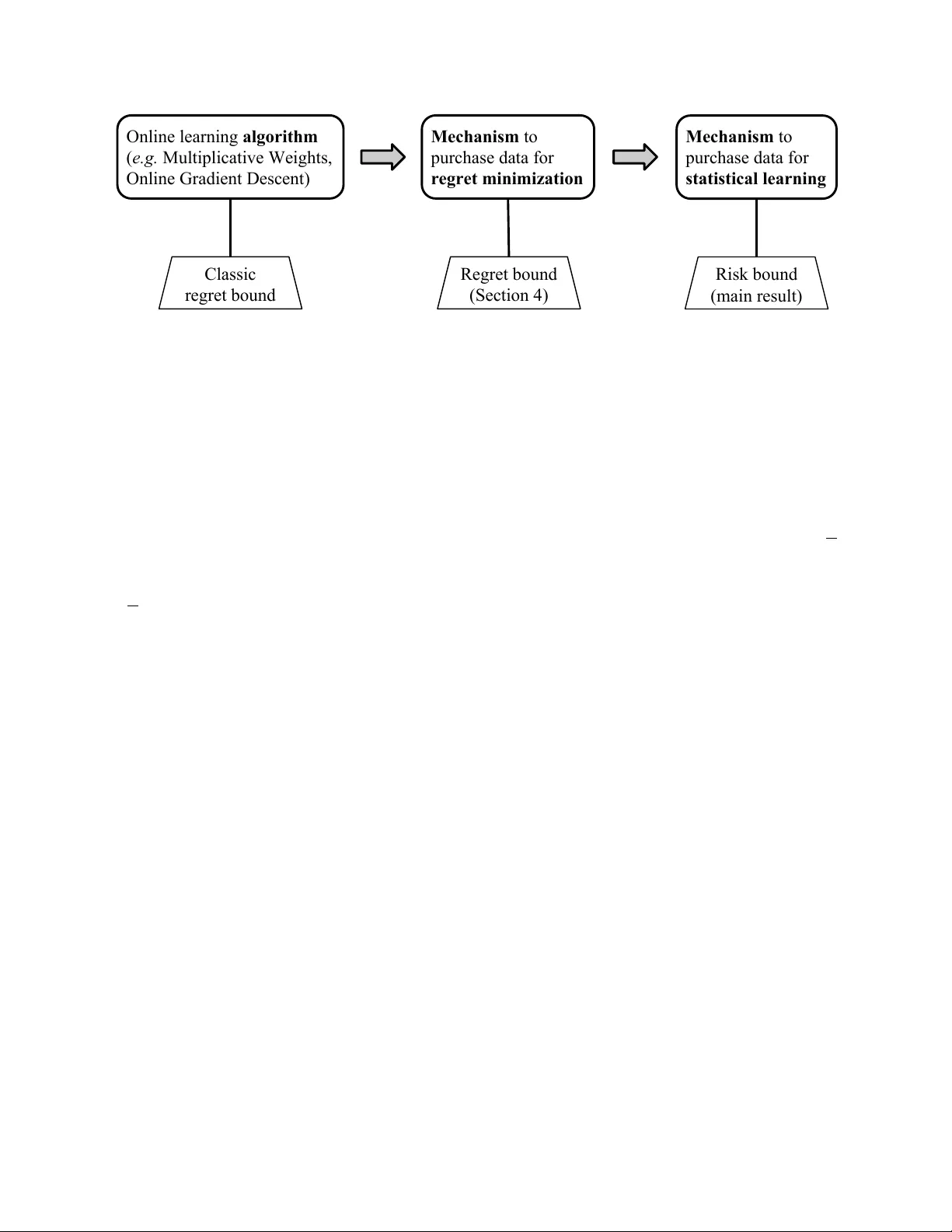
Lo w-Cost Learning via Activ e Data Pro curemen t Jacob Ab erneth y * , Yiling Chen ** , Chien-Ju Ho *** , and Bo W aggoner ** * Univ ersity of Mic higan ** Harv ard SEAS *** UCLA Ma y 2015 Abstract W e design mec hanisms for online pro curemen t of data held b y strategic agen ts for mac hine learning tasks. W e study a mo del in whic h agen ts cannot fabricate data, but ma y lie ab out their cost of furnishing their data. The challenge is to use past data to activ ely price future data in order to obtain learning guaran tees , even when agents’ costs can depend arbitrarily on the data itself. W e sho w how to con v ert a large class of no-regret algorithms in to online p osted-price and learning mechanisms. Our results parallel classic sample complexity guarantees, but with the key resource constrain t b eing money rather than quan tity of data a v ailable. With a budget constraint B , we giv e robust risk (predictive error) b ounds on the order of 1 / √ B . In many cases our guaran tees are signiﬁcan tly b etter due to an active-learning approach that leverages correlations b etw een costs and data. Our algorithms and analysis go through a model of no-regret learning with T arriving pairs (cost, data) and a budget constraint of B , coupled with the “online to batch con version”. Our regret b ounds for this mo del are on the order of T / √ B and w e give lo wer b ounds on the same order. 1 In tro duction The rising interest in the ﬁeld of Mac hine Learning (ML) has b een strongly driven b y the p oten tial to generate economic v alue. Firms seeking reven ue optimizations can gather abundan t data at low cost, apply a set of inexp ensiv e algorithmic to ols, and pro duce high- accuracy predictors that can massively impro ve future decision making. The extent of the p oten tial v alue that can b e created by lev eraging data for prediction is apparent in the m ulti-million dollar competition bounties oﬀered by companies like Netﬂix and the Heritage Health F oundation, but p erhaps even more so in the aggressive hiring of man y ML exp erts b y companies lik e Go ogle and F aceb o ok. 1 Muc h of the theoretical results in ML aim to measure, at least implicitly , the e c onomic eﬃciency of learning problems. F or example, in certain settings w e ha v e a reasonably thorough understanding of sample c omplexity [ 1 ] which gives us the precise tradeoﬀ b et ween n , the quan tity of data at our disp osal, and the error or loss rate we wan t to ac hiev e. Reducing error is alw a ys b eneﬁcial, of course, but m ust b e w eighed against the marginal cost of increasing n . The measures of eﬃciency in ML ha v e broadened in recen t years, in particular b ecause gathering data is typically orders of magnitude cheaper than labeling it. This has led to the emergence of the active le arning paradigm [ 2 – 4 , 12 , 17 ]. Here, we imagine an in terface b et w een the learner and the lab el provider, where the learner may make lab el queries on data p oin ts in an online fashion. By sequentially choosing whic h data to lab el, the learner can greatly reduce the num b er of lab els required to learn [12]. A problem that has receiv ed little attention in the learning theory literature is the monetary eﬃciency of learning when data ha ve diﬀering costs. Indeed, real-w orld prediction tasks often require obtaining examples held by self-in terested, strategic agen ts; these agents m ust b e incentivized to provide the data they hold, and they hav e heterogeneous costs for doing so. In this v ein, the presen t paper seeks to address the following question: In a w orld where data is held by self-in terested agen ts with heterogeneous costs for pro viding it, and in particular when these costs ma y b e arbitrarily correlated with the underlying data, how can w e design mec hanisms that are incen tive- compatible, hav e robust learning guarantees, and optimize the cost-eﬃciency tradeoﬀs inheren t in the learning problem? This question is relev an t to many real-w orld scenarios inv olving ﬁnancial and strategic considerations in data pro curement. Here are tw o examples: 1. In the dev elopmen t of a certain drug, a pharmaceutical compan y wishes to train a disease classiﬁer based on data obtained by hospitals and stored in patients’ medical records. These data are not public, yet the company can oﬀer hospital patients ﬁnancial incen tiv es to contribute their priv ate records. W e note the p otential for cost heterogeneit y: the comp ensation required by patients may b e correlated with the con tent of their medical data ( e.g. if they ha v e the disease). 2. Online retailers generally hop e to know more ab out website visitors in order to b etter target pro ducts to customers. A retailer can oﬀer to buy customers’ demographic and so cial data, sa y in the form of access to their F aceb o ok proﬁle. But again, customers’ willingness to sell may co v ary with their demographics data in an unknown wa y . F rom sample complexit y to budget eﬃciency The classical problem in statistical learning theory is the following. W e are giv en n datap oin ts (examples) z 1 , . . . , z n ∈ Z sampled from some distribution D . Our goal is to select a h yp othesis h ∈ H whic h “p erforms w ell” on unseen data from D . W e can specify p erformance in terms 2 of a loss function ` ( h, z ), and we write L ( h ), known as the risk of h , to b e the exp ectation of ` ( h, z ) on a random dra w z from D . The goal is to pro duce a hypothesis ¯ h whose risk is not m uch more than that of h ∗ , the optimal member of H . F or example, in binary classiﬁc ation , eac h data p oint consists of a pair z = ( x, y ) where x enco des some “features” and y ∈ {− 1 , 1 } is the lab el; a h yp othesis h is a function that predicts a lab el for a giv en set of features; and a typical loss function, the “0-1 loss”, is deﬁned so that ` ( h, ( x, y )) = 0 when h ( x ) = y and ` ( h, ( x, y )) = 1 otherwise. Researc h in statistical learning theory attempts to characterize how well suc h tasks can b e p erformed in terms of the r esour c es a v ailable and the inherent diﬃculty of the problem. The resource is usually the quantit y of data n . In binary classiﬁcation, for instance, the diﬃculty or ric hness of the problem is captured b y the “VC-dimension” d , and a famous result [ 19 ] is that there is an algorithm achieving the b ound L ( ¯ h ) ≤ L ( h ∗ ) + O r d log n n ! , (1) with v ery high probability ov er the sample z 1 , . . . , z n . In the present work w e consider an alternative scenario: the learner has a ﬁxed budget B and can use this budget to purchase examples. More precisely , on round t of a sequence of T rounds, agent t arriv es with data p oint z t , sampled i.i.d. from some D , and a cost c t ∈ [0 , 1]. This cost c t is known only to the agent and can dep end arbitrarily on z t . The learning mec hanism ma y oﬀer a (p ossibly randomized) menu of take-it-or-le ave-it prices π t : Z → R + , with a p ossibly diﬀeren t price π t ( z ) for each data p oint z . The arriving agent observ es the price π t ( z t ) oﬀered for her data and accepts as long as π t ( z t ) ≥ c t , in which case the mec hanism pa ys the agent π t ( z t ) and learns ( c t , z t ). 1 Our goal is to actively select prices to oﬀer for diﬀeren t datap oin ts, sub ject to a budget B , in order to minimize the risk of our ﬁnal output ¯ h . A t a high lev el, our main result parallels the classical statistical learning guaran tee in (1) , but where the limited resource is the budget B instead of the sample size n . Main Result 1 (Informal) . F or a lar ge class of pr oblems, ther e is an active data pur chasing algorithm A that sp ends at most B in exp e ctation and outputs a hyp othesis ¯ h satisfying, E L ( ¯ h ) ≤ L ( h ∗ ) + O  r γ T , A B  , wher e γ T , A ∈ [0 , 1] is an algorithm-dep endent p ar ameter of the (c ost, data) se quenc e c apturing the monetary diﬃcult y of learning and the exp e ctation is over the algorithm’s internal r andomness. This b ound dep ends on the quantit y γ T , A whic h captures the monetary diﬃculty of the problem at hand. (W e also need as prior knowledge a rough estimate of γ T , A .) This is in 1 W e will discuss the in teraction mo del further in Sections 2 and 8. 3 Online learning algorithm ( e.g. Multiplicative Weights, Online Gradient Descent) Classic regret bound Mechanism to purchase data for regret minimization Mechanism to purchase data for statistical learning Regret bound (Section 4) Risk bound (main result) Figure 1: Algorithmic and analytic approac h. First, w e conv ert F ollow-the-Regularized- Leader online no-regret algorithms in to mechanisms that purchase data for a regret-minimization setting that we introduce for purp oses of analysis. Then, w e con v ert these into mechanisms to solve our main problem, statistical learning. The mec hanisms interact with the online learning algorithms as blac k b o xes, but the analysis relies on “op ening the b ox”. rough analogy with VC-dimension in classical bounds suc h as Equation 1. Similarly , the key resource constrain t is now the budget B rather than the quan tit y of data n . It is imp ortant to note that γ T , A dep ends on the c hoice of algorithm A . How ev er, our results also include simpler, algorithm-indep enden t b ounds. F or instance, replace γ T , A b y √ µ , where µ is the mean of the arriving costs, and Main Result 1 con tin ues to hold (and the only prior kno wledge required is a rough estimate of µ ). But γ T , A can b e signiﬁcantly smaller than √ µ when there are particular correlations b etw een the costs and the examples; indeed, we can ha v e γ T , A → 0 ev en as µ sta ys constan t. This indicates a case in which the a verage cost of data is high, but due to b eneﬁcial correlations b et ween costs and data, our mec hanism can obtain all the data it needs for go o d learning v ery cheaply . W e give a thorough discussion of γ T , A in Section 4.4. Ov erview of T ec hniques Our general idea for attacking this problem is to utilize online learning algorithms (OLAs) for regret minimization [ 6 ]. These algorithms output a h yp othesis or prediction at each step t = 1 , . . . , T , and their p erformance is measured by the summed loss of these predictions ov er all the steps. The idea is that the hypotheses pro duced by the OLA at eac h step can b e used b oth to determine the v alue of data during the pro curement pro cess and to generate a ﬁnal prediction. In Section 3, w e la y out the to ols we need for a pricing and learning mechanism to interact with OLAs. The ﬁrst high-level problem is that, because of the budget constraint, our OLA will only see a small subset of the data sequence. W e use the to ol of imp ortanc e-weighting to giv e goo d regret-minimization guarantees even when we do not see the entire data sequence. The second problem is how to aggregate the hypotheses of the OLA and conv ert its regret guaran tee in to a risk guarantee for our statistical learning setting. This is ac hieved with the standard “online-to-batc h” con version [7]. 4 Giv en the tools of Section 3, the key remaining c hallenge is to dev elop a pricing and learning strategy that achiev es low regret. W e address this question in Section 4. W e formally deﬁne a mo del of online learning for regret minimization with purc hased data, in whic h the mec hanism must output a hypothesis at eac h time step and p erform well in hindsigh t against the en tire data sequence, but only has enough budget to purchase and observe a fraction of the arriving data. W e defer until later our detailed analysis of this setting, deriv ation of a pricing strategy , and low er b ounds. A t this p oin t, w e present our pricing strategy and regret guaran tees for this setting. In Section 5, we give our main results: risk guarantees for a learner with budget B and access to T arriving agents. These b ounds follow directly b y using the to ols in Section 3 and regret-minimization results in Section 4. In Section 6, we dev elop a deeper understanding of the regret minimization setting. W e deriv e our pricing strategy from an in-depth analysis of a more analytically tractable v ariant of the problem, the “at-cost” setting, where the mechanism is only required to pay the cost of the arriving data point rather than the price p osted. F or this setting, w e are able to deriv e the optimal pricing strategy for minimizing the regret b ound of our class of learning algorithms sub ject to an exp ected budget constrain t. W e also complement our upp er b ounds b y proving low er b ounds for data-purchasing regret minimization. These show that our mechanisms for the easier at-cost setting hav e an order-optimal regret guaran tee of T √ B γ T , A . There is a small gap to our mec hanisms for the main regret minimization setting, in which our guaran tee is on the order of T √ B √ γ T , A (recall that γ T , A ∈ [0 , 1], so this is a w eak er guarantee). The dep endence T / √ B approac hes the classic √ T regret bound when B is large (approaching T ). When B is small but still sup erconstan t, we observe the perhaps coun terintuitiv e fact that w e can ac hieve o (1) av erage regret p er arriv al while only observing an o (1) fraction of the arriving data; in other words, w e hav e “no data, no regret.” Related W ork F or “batch” settings in which all agen ts are oﬀered a price sim ultaneously , pricing sc hemes for obtaining data ha ve app eared in recent work, esp ecially Roth and Schoeneb eck [16] , whic h considered the design of mechanisms for eﬃcient estimation of a statistic. How ever, this w ork and others in related settings [ 8 , 10 , 14 ] consider oﬄine solutions, e.g. drawing a p osted price indep enden tly for all data p oints. W e focus on an active approac h in which the marginal v alue of individual examples is estimated according to the curren t learning progress and budget. A data-dep enden t approach to pricing data do es app ear in Horel et al. [13] , but that pap er fo cuses on a quite diﬀerent learning setting, a model of regression with noisy samples with a budget-feasible mec hanism design approac h. Another diﬀerence from the ab o ve pap ers is that w e prov e risk and regret b ounds rather than trying to minimize e.g. a v ariance b ound, and we also consider a broader class of learning problems. 5 Other related w ork. Other w orks suc h as Dekel et al. [9] , Ghosh et al. [11] , Meir et al. [15] fo cus on a setting in which agents may misrep ort their data (also see the p eer-prediction literature). W e supp ose that agen ts ma y misrep ort their costs but not their data. Man y of the ideas in the presen t work draw from recent adv ances in using imp ortance w eighting for the active learning problem [ 4 ]. There is a wealth of theoretical researc h into activ e learning, including Balcan et al. [2] , Beygelzimer et al. [5] , Hanneke [12] and many others. “Budgeted Learning” is a somewhat related area of machine learning, but there the budget is not monetary . The idea is that we do not see all of the features of the data p oin ts in our set, but rather hav e a “budget” of the num b er of features we may observe (for instance, we ma y choose an y tw o of the three features height, weigh t, age). 2 Statistical Learning with Purc hased Data In this section, w e formally deﬁne the problem setting. The b o dy of the pap er will then consist of a series of steps for deriving mec hanisms for this setting with pro v able guaran tees, whic h will ﬁnally app ear in Section 5. W e consider a statistical learning problem describ ed as follo ws. Our data points are ob jects z ∈ Z . W e are given a h yp othesis class H whic h w e will assume is parameterized b y vectors R d but more broadly can b e an y Hilb ert space endo wed with a norm k · k ; for con venience we will treat elemen ts h ∈ H as vectors which can b e added, scaled, etc. W e are also giv en a loss function ` : H × Z → R that is conv ex in H . W e assume throughout the pap er that the loss function is 1-Lipschitz in h ; that is, for any z ∈ Z and an y h, h 0 ∈ H w e ha ve | ` ( h, z ) − ` ( h 0 , z ) | ≤ k h − h 0 k . In man y common scenarios, Z is the space of pairs ( x, y ) from the cross pro duct X × Y , with x the feature input and y the lab el, though in our setting Z can b e a more generic ob ject. F or example, in the canonical problem of line ar r e gr ession , we ha v e that Z = X × Y = R d × R , the hypothesis class is v ectors H = R d , and the loss function is deﬁned according to squared error ` ( h, ( x, y )) := ( h > x − y ) 2 . The data-purc hasing statistical learning problem is parameterized by the data space Z , hypothesis space H , loss function ` , num b er of arriving data p oin ts T , and exp ected budget constrain t B . A pr oblem instanc e consists of a distribution D on the set Z and a sequence of pairs ( c 1 , z 1 ) , . . . , ( c T , z T ) where each z t is a data p oin t dra wn i.i.d. according to D and eac h c t ∈ [0 , 1] is the priv ate cost asso ciated with that data point. The costs may b e arbitrarily chosen, i.e. w e consider a worst-case mo del of costs. (F or instance, if costs and data are drawn together from a joint, correlated distribution, then this is a sp ecial case of our setting.) In this problem, the task is to design a me chanism implementing the op erations “p ost”, “receiv e”, and “predict” and interacting with the problem instance as follo ws. • F or eac h time step t = 1 , . . . , T : 6 1. The mec hanism p osts a pricing function π t : Z → R , where π t ( z ) is the price p osted for data p oint z . 2. Agen t t arriv es, p ossessing ( c t , z t ). 3. If the posted price π t ( z t ) ≥ c t , then agen t t accepts the transaction: The mechanism pa ys π t ( z t ) to the agent and r e c eives ( c t , z t ). If π t ( z t ) < c t , agen t t rejects the transaction and the mechan ism r e c eives a null signal. • The mechanism outputs a pr e diction ¯ h ∈ H . Note that the mec hanism is given the parameters Z , H , ` , T , and B , but the problem instance is completely unkno wn to the mec hanism prior to to the arriv als. The design problem of the mec hanism is how to choose the pricing function π t to p ost at each time, how to up date based on r e c eiving data, and how to choose the ﬁnal pr e diction . The risk or predictiv e error of a h yp othesis is L ( h ) = E z ∼D ` ( h, z ) and the goal of the mec hanism is to minimize the risk L ( ¯ h ) of its ﬁnal hypothesis ¯ h . The b enc hmark is the optimal hypothesis in the class, h ∗ = arg min h ∈H L ( h ). The mechanism must guaran tee that, for every input sequence ( c 1 , z 1 ) , . . . , ( c T , z T ), it sp ends at most B in exp ectation ov er its o wn internal randomness. Agen t-mechanism in teraction. The mo del of agent arriv al and p osted prices contains sev eral assumptions. First, agen ts cannot fabricate data; they can only rep ort data they actually ha v e to the mec hanism. Second, agents are rational in that they accept a p osted price when it is higher than their cost and reject otherwise. Third, we ha ve an implemen tation of the mec hanism that can obtain the agent’s cost c t when the transaction o ccurs. W e emphasize that the purp ose of this pap er is not fo cused on the implementation of suc h a setting, but instead on developing active learning and pricing tec hniques and guarantees. This is also in tended as a simple and clean mo del in whic h to begin developing such tec hniques. Ho wev er, we brieﬂy note some p ossible implementations. In the most straightforw ard one, the mechanism p osts prices directly to the agen t who resp onds directly . This would b e a w eakly truthful implementation, as agen ts hav e no incen tive to misrep ort costs after they choose to accept the transaction. One strictly truthful implementation uses a truste d thir d p arty (TTP) that can facilitate the transactions (and guaran tee the v alidity of the data if necessary). F or example, w e could imagine attempting to learn to classify a disease, and w e could rely on a hospital to act as the brok er allowing us to negotiate with patients for their data. Then the TTP/agent interaction could pro ceed as follows: 1. Learning mechanism submits the pricing function π t to the TTP; 2. Agen t pro vides his data p oin t z t and cost c t to the TTP; 7 3. TTP determines whether π t ( z t ) ≥ c t and, if so, instructs the learner to pay π t ( z t ) to the agen t and then provides the pair ( z t , c t ) to the learner. Other p ossibilities for strictly truthful implementation include using a bit of cryptograph y (see Section 8). 3 T o ols for Con v erting Regret-Minimizing Algorithms In this section we b egin with the classic regret-minimization problem and a broad class of algorithms for this problem. W e then show ho w to apply techniques that conv ert these algorithms into a form that will b e useful for solving the statistical learning problem with purc hased data. The only missing ingredien t will then b e a price-p osting strategy , which will b e presented in Section 4. 3.1 Recap of Classic Regret-Minimization In the classic regret-minimization problem, w e hav e a h yp othesis class H with the same assumptions as stated in Section 2. A t eac h time t = 1 , . . . , T the algorithm posts a h yp othesis h t ∈ H . Nature (the adv ersary , the en vironment, etc.) selects a 1-Lipsc hitz conv ex loss function f t : H → R . 2 The algorithm observ es f t and suﬀers loss f t ( h t ). The loss and r e gr et of the algorithm on this particular input sequence are Loss T = T X t =1 f t ( h t ) . (2) Regret T = Loss T − min h ∗ ∈H T X t =1 f t ( h ∗ ) . (3) The regret ob jective is what one typically studies in adv ersarial settings, where w e wan t to discoun t the loss incurred b y the algorithm b y the loss suﬀered by the b est p ossible h ∗ c hosen with kno wledge of the sequence of f t ’s. As we often consider randomized algorithms, we will generally consider exp e cte d loss and regret, where the exp ectation is o ver any randomness in the algorithm not ov er the (p ossibly-randomized) input sequence of loss functions. An algorithm is said to guarantee regret R ( T ) if the latter provides an upp er b ound on regret for ev ery sequence of loss functions f 1 , . . . , f T . W e utilize the broad class of F ol low-the-R e gularize d-L e ader (FTRL) online algorithms (Algorithm 1) [ 18 , 20 ]. Sp ecial cases of FTRL include Online Gradient Descen t, Multiplicativ e W eights, and others. Each FTRL algorithm is sp eciﬁed by a con vex function G : H → R whic h is known as a r e gularizer and is usually strongly conv ex with resp ect to some norm. F or example, Multiplicative W eigh ts follo ws by using the negativ e entrop y function as a 2 This deﬁnition of “loss function” is a departure from our main setting which inv olved ` ( · , · ). But we will use this somewhat more general setup by choosing f t ( h ) ∝ ` ( h, z t ) for the datap oint z t . 8 regularizer, which is strongly-conv ex with resp ect to ` 1 norm [ 6 ]. Online Gradient Descen t follo ws by using the regularizer G ( h ) = 1 2 k h k 2 2 , which is strongly-con v ex with resp ect to ` 2 norm. These sp ecial cases ha v e eﬃcien t closed-form solutions to the up date rule for computing h t +1 . ALGORITHM 1: F ollo w-the-Regularized-Leader (FTRL). Input : learning parameter η , con v ex regularizer G : H → R for t = 1 , . . . , T do p ost hypothesis h t , observ e loss function f t ; up date h t +1 = inf h ∈H n P t 0 ≤ t f t 0 ( h ) + η G ( h ) o ; end It is well-kno wn (and indeed follows as a special case of Lemma 3.1) that, under the assumptions on our setting, FTRL algorithms guarantee an exp ected regret b ound of O ( √ T ), and this is tight with resp ect to T . 3.2 Imp ortance-W eigh ting T ec hnique for Less Data As a starting p oin t, supp ose we wish to design an online learning algorithm that do es not observ e all of the arriving loss functions, but still performs well against the entire arriv al sequence. Because the arriv al sequence may b e adv ersarially c hosen, a go o d algorithm should randomly choose to sample some of the arriv als. In this section, we abstract aw a y the decision of ho w to randomly sample. (This will b e the fo cus of Section 4.) In this section, we supp ose that at each time t , after p osting a hypothesis h t , a probability q t > 0 is sp eciﬁed by some external means as a (p ossibly random) function of the preceding time steps. With probability q t , w e observ e f t ; with probabilit y 1 − q t , w e observ e nil. Our goal is to mo dify the FTRL algorithm for this setting and obtain a mo diﬁed regret guaran tee. Notice crucially that the deﬁnition of loss and regret (3) are unchanged: W e still suﬀer the loss f t ( h t ) regardless of whether we observ e f t . The key technique w e use is imp ortanc e weighting . The idea is that, if we only observ e eac h of a sequence of v alues x i with probabilit y p i , then w e can get an unbiased estimate of their sum b y taking the sum of x i p i for those w e do observ e. T o c heck this fact, let 1 i b e the indicator v ariable for the even t that w e observe i and note that the exp ectation of our sum is E h P i 1 i x i p i i = P i x i . This is called imp ortance-w eighting the observ ations (and is a speciﬁc instance of a more general machine learning technique). F urthermore, if each x i p i is b ounded and observ ed independently , we can exp ect the estimate to b e quite go o d via tail b ounds. The imp ortance-w eighted mo diﬁcation to an online learning algorithm is outlined in Algorithm 2. The imp ortance-weigh ted regret guarantee w e obtain is given in Lemma 3.1. It dep ends on the following k ey notation. Our analysis and algorithm require a giv en norm k · k , and we recall the deﬁnition of the dual norm k z k ? := sup x ; k x k≤ 1 x · z . 9 Deﬁnition 3.1. Given h ∈ H , and conv ex loss f : H → R , let ∆ h,f := k∇ f ( h ) k ? . W e can informally think of ∆ h,f b oth as the “diﬃcult y” of arriv al f when the curren t h yp othesis is h , and as the “v alue” of observing f . This interpretation is explored in Section 4 when w e deﬁne the parameter γ T , A . ALGORITHM 2: Importance-W eighted Online Learning Algorithm. Input : access to Online Learning Algorithm (OLA) for t = 1 , . . . , T do p ost hypothesis h t ← OLA; observ e sampling probabilit y q t ; toss q t -w eighted coin (Bernoulli sample)  t ; if  t = ( 1 input imp ortance-weigh ted loss function ˆ f t ( · ) = f t ( · ) q t → OLA 0 input zero function ˆ f t ( · ) ≡ 0 → OLA end Lemma 3.1. Assume we implement Algorithm 2 with nonzer o sampling pr ob abilities q 1 , . . . , q T . Assume the underlying OLA is FTRL (Algorithm 1) with r e gularizer G : H → R that is str ongly c onvex with r esp e ct to k · k . Then the exp e cte d r e gr et, with r esp e ct to the loss se quenc e f 1 , . . . , f T , is no mor e than R ( T ) = β η + 2 η E h P T t =1 ∆ 2 h t ,f t q t i , wher e β is a c onstant dep ending on H and G , η is a p ar ameter of the algorithm, and the exp e ctation is over any r andomness in the choic es of h t and q t . W e can recov er the classic regret b ound as follows: T ake each q t = 1, and note b y the Lipsc hitz assumption that each ∆ h t ,f t ≤ 1. Then by setting η = Θ(1 / √ T ), we get an exp ected regret b ounded by O ( √ T ). 3.3 The “Online-to-Batc h” Con v ersion So far so go o d: W e can con vert an online regret-minimization algorithm to use smaller amoun ts of data, and we p ostp one the question of how to price data till Section 4. W e now address the statistical learning problem, which is ho w to generate accurate pr e dictions based on the online learning pro cess. W e address this with a standard to ol known as the “online-to-batch con version,” where w e may leverage an online learning algorithm for use in a “batch” setting. A sketc h of this tec hnique is as follows, and further details can b e found in, e.g., Shalev-Shw artz [18] . Giv en a batch of i.i.d. data p oin ts, feed them one-by-one into the no-regret algorithm. Because the algorithm has lo w regret, its hypotheses predicted well on av erage. But since each data p oint w as drawn i.i.d., this means that these hypotheses on av erage predict well on an i.i.d. dra w from the distribution. Thus it suﬃces to tak e the mean of the hypotheses to obtain lo w risk. 10 Lemma 3.2 (Online-to-Batc h [ 7 ]) . Supp ose the se quenc e of c onvex loss functions f 1 , . . . , f T ar e dr awn i.i.d. fr om a distribution F and that an online le arning algorithm with hyp otheses h 1 , . . . , h T achieves exp e cte d r e gr et R ( T ) . L et L ( h ) = E f ∼F f ( h ) and h ∗ = arg min h ∈H L ( h ) . F or ¯ h 1: T = 1 T P T t =1 h t , we have E f 1 ,...,f T , alg L ( ¯ h 1: T ) ≤ L ( h ∗ ) + 1 T R ( T ) . W e note that this con version will contin ue to hold in the data-purchasing no-regret setting w e deﬁne next, since all that is required is that the algorithm output a h yp othesis h t at each step and that there is a regret b ound on these hypotheses. 4 Regret Minimization with Purc hased Data In this setting, we deﬁne the problem of regret minimization with purchased data. W e will design mechanisms with go o d regret guaran tees for this problem, whic h will translate via the aforemen tioned online-to-batc h conv ersion (Lemma 3.2) into guarantees for our original problem of statistical prediction. The essence of the data-purchasing no-regret learning setting is that an online algorithm (“mec hanism”) is asked to p erform w ell against a sequence of data, but by default, the mec hanism do es not hav e the abilit y to see the data. Rather, the mec hanism may purc hase the righ t to observe data p oints using a limited budget. The mechanism is still exp ected to ha ve low regret compared to the optimal h yp othesis in hindsigh t on the entire data sequence (ev en though it only observes a p ortion of the sequence). 4.1 Problem Deﬁnition The data-purc hasing regret minimization problem is parameterized by the hypothesis space H , num b er of arriving data p oin ts T , and exp ected budget constraint B . A pr oblem instanc e is a sequence of pairs ( c 1 , f 1 ) , . . . , ( c T , f T ) where each f t : H → R is a conv ex loss function and each c t ∈ [0 , 1] is the cost asso ciated with that data p oin t. W e assume that the f t are 1-Lipsc hitz, and let F b e the set of such loss functions. In this problem, w e design a me chanism implemen ting the op erations “p ost” and “receive” and in teracting with the problem instance as follo ws. • F or eac h time step t = 1 , . . . , T : 1. The mechanism p osts a hypothesis h t and a pricing function π t : F → R , where π t ( f ) is the price p osted for loss function f . 2. Agen t t arriv es, p ossessing ( c t , f t ). 3. If the posted price π t ( f t ) ≥ c t , then agen t t accepts the transaction: The mec hanism pa ys π t ( f t ) to the agen t and r e c eives ( c t , f t ). If π t ( f t ) < c t , agen t t rejects the transaction and the mechan ism r e c eives a null signal. 11 Note the k ey diﬀerences from the statistical learning setting: W e must p ost a h yp othesis h t at each time step (and w e do not output a ﬁnal prediction), and data is not assumed to come from a distribution. The goal of the mechanism is to minimize the loss, namely P t f t ( h t ). The deﬁnition of regret is also the same as in the classical setting (Equation 3). Note that we suﬀer a loss f t ( h t ) at time t regardless of whether we purchase f t or not. The mechanism must also guaran tee that, for every problem instance ( c 1 , f 1 ) , . . . , ( c T , f T ), it sp ends at most B in exp ectation ov er its o wn in ternal randomness. 4.2 The Imp ortance-W eigh ting F ramew ork Recall that, in Section 3.2, we introduced the imp ortanc e-weighting technique for online learning. This ga ve regret guarantees for a learning algorithm when each arriv al f t is observed with some probabilit y q t . Our general approac h will b e to develop a strategy for randomly drawing p osted prices π t . This will induce a probability q t of obtaining eac h arriv al f t . Therefore, the en tire problem has b een reduced to choosing a p osted-price strategy at eac h time step. This posted-price strategy should attempt to minimize the regret b ound while satisfying the exp ected budget constraint. A brief sketc h of the pro of arguments is as follows. After w e c ho ose a p osted price strategy , eac h q t will b e determined as a function of h t , c t , and f t . ( q t is just equal to the probabilit y that our randomly dra wn price exceeds the agen t’s cost c t .) Thus, w e can apply Lemma 3.1, whic h stated that for these induced probabilities q t , the exp ected regret of the learning algorithm is β η + 2 η E X t ∆ 2 h t ,f t q t , where β is a constant and η is a parameter of the learning algorithm to b e chosen later. After w e c ho ose and apply such a strategy , the general approach to proving our regret b ounds is to ﬁnd an a priori b ound M suc h that 2 E P t ∆ 2 h t ,f t q t ≤ M . Then the regret b ound b ecomes β η + η M . If we know this upp er-b ound M in adv ance using some prior knowledge, then we can c ho ose η = Θ(1 / √ M ) as the parameter for our learning algorithms. This giv es a regret guaran tee of O ( √ M ). 4.3 A First Step to Pricing: The “A t-Cost” V arian t The bulk of our analysis of the no-regret data-purchasing problem actually fo cuses on a sligh tly easier v ariant of the setting: If the arriving agent accepts the transaction, then the mec hanism only has to pa y the cost c t rather than the p osted price π t ( f t ). W e call this the “at-cost” v ariant of the problem. This setting turns out to b e muc h more analytically tractable: W e deriv e optimal regret b ounds for our mechanisms and matc hing low er b ounds. W e then tak e the k ey approac h and insights derived from this v ariant and apply them to 12 pro duce a solution to the main no-regret data purc hasing problem. In order to keep the story mo ving forw ard, we summarize our results for the “at-cost” setting here and explore how they are obtained in Section 6. In the at-cost setting, we are able to solve directly for the pricing strategy that minimizes the imp ortance-weigh ted regret b ound of Lemma 3.1. W e ﬁrst deﬁne one important quantit y , then w e state the strategy and result in Theorem 4.1. Deﬁnition 4.1. F or a ﬁxed input sequence ( c 1 , f 1 ) , . . . , ( c T , f T ), ∆ h,f in Deﬁnition 3.1, and a mec hanism outputting (p ossibly random) hypotheses h 1 , . . . , h T , deﬁne γ T , A = E 1 T X t ∆ h t ,f t √ c t where the exp ectation is ov er the randomness of the algorithm. Note that γ T , A lies in [0 , 1] b y our assumptions on b ounded cost and Lipschitz loss. No w we give the main result for the at-cost setting. Theorem 4.1. Ther e is a me chanism for the “at-c ost” pr oblem of data pur chasing for r e gr et minimization that interfac es with FTRL and guar ante es to me et the exp e cte d budget c onstr aint, wher e for a p ar ameter γ T , A ∈ [0 , 1] (Deﬁnition 4.1), 1. The exp e cte d r e gr et is b ounde d by O  max n T √ B γ T , A , √ T o . 2. This is optimal in that no me chanism c an impr ove b eyond c onstant factors. 3. The pricing str ate gy is to cho ose a p ar ameter K = O  T B γ T , A  and dr aw π t ( f ) r andomly ac c or ding to a distribution such that Pr[ π t ( f ) ≥ c ] = min n 1 , ∆ h t ,f K √ c o . The only prior know le dge r e quir e d is an estimate of γ T , A up to a c onstant factor. 4.4 In terpreting the Quan tit y γ T , A Sev eral of our b ounds rely heavily on the quan tity γ T , A whic h measures, in a sense, the “ﬁnancial diﬃculty” of the problem. W e no w devote some discussion to understanding γ T , A b y answering four questions. (1) How to interpr et γ T , A ? γ T , A is an a verage, o v er time steps t , of ∆ h t ,f t · √ c t . Here, ∆ h t ,f t in tuitively captures b oth the “diﬃcult y” of the data f t and also the “v alue” or “b eneﬁt” of f t . T o explain the diﬃcult y asp ect, b y examining the regret bound for FTRL learning algorithms ( e.g. the imp ortance-w eigh ted regret b ound of Lemma 3.1 with all q t = 1), one observ es that if each ∆ h t ,f t is small, then we ha ve an excellent regret b ound for our learning algorithm; the problem is “easy”. T o explain the v alue aspect, one can for concreteness tak e the Online Gradien t Descen t algorithm; the larger the gradien t, the larger the up date at this step, and ∆ h t ,f t 13 is the norm of the gradient. And in general, the higher ∆ h t ,f t , the more lik ely w e are to purc hase arriv al f t . Th us, γ T , A captures the correlations b etw een the v alue of the arriving data and the cost of that data. If either the mean of the costs or the a verage b eneﬁt ∆ h t ,f t of the data is con verging to 0, then γ T , A → 0 and in these cases w e can learn with high accuracy v ery c heaply , as may b e exp ected. More interestingly , it is p ossible to ha ve b oth high av erage costs, and high av erage data-v alues, and y et still hav e γ T , A → 0 due to b eneﬁcial correlations. In these cases w e can learn m uc h more c heaply than might b e exp ected based on either the economic side or the learning side alone. (2) When should we exp e ct to have go o d prior know le dge of γ T , A ? Although in general γ T , A will b e domain-sp eciﬁc, there are several reasons for optimism. First, γ T , A compresses all information ab out the data and costs into a single scalar parameter (compare to the common mec hanism-design assumption that the prior distribution of agents’ v alues is fully known). Second, we do not need very exact estimates of γ T , A ( e.g. we do not need to know γ T , A ±  ): F or order-optimal regret b ounds, we only need an estimate within a constan t factor of γ T , A . Third, γ T , A is directly prop ortional to K , whic h is a normalization constan t in our pricing distribution: If w e increase K , the probabilit y of obtaining a giv en data p oin t only decreases, and vice v ersa. In fact, the b est c hoice of K is the normalization constan t so that we run out of budget precisely when the last arriv al leav es. Thus, K (equiv alen tly , γ T , A ) can b e estimated and adjusted online by tracking the “burn rate” (sp ending p er unit time) of the algorithm. In simulatio ns, w e ha ve observ ed success with a simple approach of estimating K based on the a verage correlation so far along with the burn rate, i.e. if the curren t estimated γ T , A is ˆ γ T , A and there are ˆ T steps remaining with ˆ B budget remaining to sp end, set K = ˆ γ T , A ˆ T / ˆ B . (3) What c an we pr ove without prior know le dge of γ T , A ? It turns out that, if we only hav e an estimate of ¯ c = 1 T P t √ c t , resp ectively µ = 1 T P t c t , then this suﬃces for regret guaran tees on the order of T ¯ c/ √ B , resp ectively T √ µ/ √ B . This “graceful degradation” will con tinue to b e true in the main setting. The idea is that we can follo w the optimal form of the pricing strategy while c ho osing an y normalization constant K ≥ T B γ T , A . It may no longer b e optimal, but it will ensure that we satisfy the budget and giv e guarantees dep ending on the magnitude of K . So all we need is an approximate estimate of some v alue larger than γ T , A . Both ¯ c and µ are guaran teed to upp er-b ound on γ T , A , so b oth can b e used to pic k K while satisfying the budget. T o recap, kno wledge of only a simple statistic such as the mean of the arriving costs suﬃces for go o d learning guarantees, with b etter kno wledge translating to better guaran tees. (4) γ T , A dep ends on the algorithm—what ar e the implic ations? W e ﬁrst note that γ T , A can b e upp er-b ounded by , for instance, √ µ where µ is the a v erage of the arriving costs. So a b ound containing γ T , A do es imply nontrivial algorithm-indep endent b ounds. The purp ose of γ T , A is to capture cases where w e can do signiﬁcantly b etter than suc h b ounds b ecause the algorithm is a go o d ﬁt for the problem. T o see this, note that running the FTRL algorithm on the entire data sequence (with no budget constraint) giv es a 14 regret b ound of β η + η P T t =1 ∆ 2 h t ,f t . The w orst case has eac h ∆ h t ,f t equal to 1, pro ducing a √ T regret b ound. But in a case where the algorithm has a small av erage ∆ h t ,f t and the algorithm enjo ys a better regret bound, we may also hop e that this improv emen t is reﬂected in γ T , A . Ho wev er, one might hop e for an algorithm-indep enden t quantit y that, in analogy with V C-dimension, captures the “diﬃcult y” of the purc hasing and learning problem instance. This leads to the question: (4a) Can we r emove the algorithm-dep endenc e of the b ound? One migh t hop e to achiev e a b ound dep ending on an algorithm-indep endent quantit y that captures correlations b etw een data and cost. A natural candidate is γ ∗ T , A := 1 T P t ∆ h ∗ ,f t √ c t . In general, there are diﬃcult cases where one can not achiev e a b ound in terms of γ ∗ T , A . How ever, in nicer scenarios we ma y expect γ T , A to appro ximate γ ∗ T , A . F or instance, supp ose ` ( h, z ) = φ ( h > z ) where φ is a diﬀerentiable conv ex function whose gradient is 1-Lipschitz — commonly-used examples include the squar e d hinge loss and the lo g loss . Under this condition, where again w e are using f t ( · ) := ` ( · , z t ), w e can show that ∆ h t ,f t √ c t − ∆ h ∗ ,f t √ c t = k∇ ` ( h t , z t ) k ? √ c t − k∇ ` ( h ∗ , z t ) k ? √ c t ≤ k ( φ 0 ( h > t z t ) − φ 0 ( h ∗> z t )) z t k ? ≤ | φ ( h > t z t ) − φ ( h ∗> z t ) | = | ` ( h t , z t ) − ` ( h ∗ , z t ) | . By the regret guarantee of our mechanism when run with a go o d algorithm, even initialized with v ery w eak kno wledge, this diﬀerence in losses p er time step is o (1), implying that γ T , A → γ ∗ T , A . A deep er in v estigation of this phenomenon is a go o d candidate for future work. 4.5 Mec hanisms and Results for Regret Minimization In the previous section, w e presen ted our results for the easier “at-cost” v arian t. W e now apply the approac h deriv ed for that setting to the main regret minimization problem. F or this problem, unlik e in the “at-cost” v ariant, w e cannot in general solv e for the form of the optimal pricing strategy . This is intuitiv ely b ecause, when we must pay the price we p ost, the optimal strategy dep ends on c t . But the algorithm cannot condition the purc hasing decision directly on c t , as this is priv ate information of the arriving agent. W e prop ose simply drawing p osted prices according to the optimal strategy derived for the at-cost setting, namely , Pr[ π t ( f ) ≥ c ] = min  1 , ∆ h t ,f K √ c  , (4) but with a diﬀeren t c hoice of normalization constan t K . W e note that there is a pricing distribution that accomplishes this: Observ ation 1. F or any K and ∆ h t ,f , ther e exists a pricing distribution on π t ( f ) that satisﬁes Equation 4. L etting c ∗ = ∆ 2 h t ,f /K 2 , the CDF is given by F ( π ) = Pr [ π t ( f ) ≤ π ] = 0 if π ≤ c ∗ , F ( π ) = 1 − ∆ h t ,f /K √ π if c ∗ ≤ π ≤ 1 , and F ( π ) = 1 if π > 1 . 15 0 c ∗ 1 price π 0 1 /c ∗ PDF (a) Probability densit y function of the pricing dis- tribution. The price π ( f ) = 1 with probabilit y min { 1 , ∆ h t ,f /K } . On the in terv al ( c ∗ , 1) the den- sit y function is x 7→ ∆ h t ,f / 2 K x 3 / 2 . 0 c ∗ 1 price π 0 1 − ∆ h t ,f /K 1 CDF (b) Cumulativ e distribution function of the pricing distribution. Equal to zero for π ≤ c ∗ , then equal to 1 − ∆ h t ,f /K √ π on ( c ∗ , 1), then equal to 1 at cost 1. Figure 2: The pricing distribution. Illustrates the distribution from whic h we dra w our p osted prices at time t , for a ﬁxed arriv al f . The quantit y ∆ h t ,f captures the “b eneﬁt” from obtaining f . K is a normalization parameter. The distribution’s supp ort has a lo west price c ∗ , whic h has the form c ∗ = ∆ 2 h t ,f t /K 2 . The pricing distribution is given in Figure 2. This strategy gives Mechanism 3. As in the known-costs case, our regret b ounds dep end up on the prior knowledge of the algorithm. It will turn out to b e helpful to hav e prior knowledge ab out b oth γ T , A and the follo wing parameter, whic h can b e interpreted as γ T , A with all costs c t = 1: γ max T , A = E 1 T X t ∆ h t ,f t . Theorem 4.2. If Me chanism 3 is run with prior know le dge of γ T , A and of γ max T , A (up to a c onstant factor), then it c an cho ose K and η to satisfy the exp e cte d budget c onstr aint and obtain a r e gr et b ound of O  max  T √ B g , √ T  , wher e g = p γ T , A · γ max T , A (by setting K = T B γ max T , A ). Similarly, know le dge only of γ T , A , r esp e c- tively ¯ c = 1 T P t √ c t , r esp e ctively µ = 1 T P t c t suﬃc es for the r e gr et b ound with g = √ γ T , A , r esp e ctively g = √ ¯ c , r esp e ctively g = µ 1 / 4 . W e can observ e a quantiﬁable “price of strategic behavior” in the diﬀerence b et ween the regret guaran tees of Theorems 4.2 (this setting) and Theorem 4.1 (the “at-cost”) setting: T √ B q γ T , A · γ max T , A vs T √ B γ T , A . Note that γ max T , A ≥ γ T , A , and they approach equality as all costs approach the upp er b ound 1, but b ecome very diﬀerent as the av erage cost µ → 0 while the maximum cost remains ﬁxed at 1. 16 Mec hanism 3: Mechanism for no-regret data-purchasing problem. Input : parameters K , η , access to online learning algorithm (OLA) set OLA parameter η ; for t = 1 , . . . , T do p ost hypothesis h t ← OLA; p ost prices π t ( f ) drawn randomly suc h that Pr[ π t ( f ) ≥ c ] = min n 1 , ∆ h t ,f K √ c o ; if we receive ( c t , f t ) then let q t = Pr π t [ π t ( f t ) ≥ c t ]; let imp ortanc e-weighte d loss function ˆ f t ( · ) = f t ( · ) q t ; send ˆ f t → OLA; else send 0 function → OLA; end end Comparison to low er b ound. Our low er-b ound for the data purchasing regret minimiza- tion problem is Ω  T √ B γ T , A  (follo ws from the low er b ound for the at-cost setting, Theorem 6.2). So the diﬀerence in b ounds discussed ab ov e, a factor of p γ max T , A v ersus √ γ T , A , is the only gap b etw een our upp er and low er b ounds for the general data purc hasing no regret problem. The most immediate op en problem in this pap er is close this gap. Intuitiv ely , the lo w er b ound do es not take adv an tage of “strategic b ehavior” in that a p osted-price mec hanism ma y often ha v e to pa y signiﬁcan tly more than the data actually costs, meaning that it obtains less data in the long run. Mean while, it may b e possible to improv e on our upp er-b ound strategy b y drawing prices from a diﬀeren t distribution. 5 Results for Statistical Learning In this section, we give the ﬁnal mechanism, Mechanism 4, for the data purc hasing statistical learning problem. The idea is to simply run the regret-minimization Mec hanism 3 on the arriving agen ts. A t eac h stage, Mechanism 3 p osts a hypothesis h t . W e then aggregate these h yp othesis b y a veraging to obtain our ﬁnal prediction. Mec hanism 4: Mechanism for statistical learning data-purchasing problem. Input : parameters K, η , access to OLA iden tify each data p oin t z with the loss function f ( · ) = ` ( · , z ); run Mec hanism 3 with parameters η , K and access to OLA; let h 1 , . . . , h T b e the resulting hypotheses; output ¯ h = 1 T P t h t ; 17 Theorem 5.1. Me chanism 4 guar ante es sp ending at most B in exp e ctation and E L ( ¯ h ) ≤ L ( h ∗ ) + O  max n g √ B , q 1 T o , wher e g = p γ T , A · γ max T , A , assuming that γ T , A and γ max T , A ar e known in advanc e up to a c onstant factor. If one assumes appr oximate know le dge r esp e ctively of γ T , A , of ¯ c = 1 T P t √ c t , or of µ = 1 T P t c t , then the guar ante e holds with r esp e ctively g = √ γ T , A , g = √ ¯ c , or g = µ 1 / 4 . Pr o of. By Theorem 4.2, Mec hanism 3 guaran tees an exp ected regret of O  max n T √ B g , √ T o when run with the sp eciﬁed prior kno wledge for the sp eciﬁed v alues of g . Therefore, the online-to-batc h conv ersion of Lemma 3.2 prov es the theorem. The statement of Main Result 1 is the special case where only γ T , A is known and g = √ γ T , A . A detailed discussion of γ T , A is in Section 4.4. 6 Deriving Pricing and the “at-cost” V arian t In Section 4.3, we stated our results for the easier at-cost v ariant of the regret minimization with purchased data problem. This included the p osted-price distribution that we use for our main results. In this section, we show how these results and this distribution are deriv ed. The “at-cost” v arian t is formally deﬁned in exactly the same w ay as the main setting, except that when π t ≥ c t and the transaction o ccurs, the mechanism only pays the cost c t rather than the p osted price π t . W e ﬁrst sho w ho w our p osted-price strategy is deriv ed as the optimal solution to the problem of minimizing regret sub ject to the budget constrain t. The resulting upp er b ounds for the “at-cost” v arian t w ere giv en in Theorem 4.1. Then, we give some fundamental low er b ounds on regret, showing that in general our upp er b ounds cannot b e improv ed up on here. These lo wer b ounds also hold for the main no-regret data purchasing problem, where there is a small gap to the upp er b ounds. 6.1 Deriving an Optimal Pricing Strategy W e b egin by asking what seems to b e an even easier question. Supp ose that for every pair ( c t , f t ) that arrives, w e could ﬁrst “see” ( c t , f t ), then choose a probability with which to obtain ( c t , f t ) and pa y c t . What w ould b e the optimal probabilit y with which to take this data? Lemma 6.1. T o minimize the r e gr et b ound of L emma 3.1, the optimal choic e of sampling pr ob ability is of the form q t = min { 1 , ∆ h t ,f t /K ∗ √ c t } . The normalization factor K ∗ ≈ T B γ T , A . The proof follows by form ulating the conv ex programming problem of minimizing the regret b ound of Lemma 3.1 sub ject to an exp ected budget constrain t. It also giv es the form of 18 the normalization constant K ∗ , which dep ends on the input data sequence and the hypothesis sequence. The k ey insigh t is no w that we can actually ac hieve the sampling probabilities dictated by Lemma 6.1 using a randomized p osted-price mechanism. Notice that these optimal sampling probabilities are decreasing in c t . In general, when drawing a price from some distribution, the probability that it exceeds c will b e decreasing in c . So it only remains to ﬁnd the p osted-price distribution that actually induces the sampling probabilities that w e wan t for all c sim ultaneously . That is, by randomly drawing p osted prices according to our distribution, w e choose to purchase ( c t , f t ) with exactly the probabilit y q t stated in Lemma 6.1, for an y p ossible v alue of c t and without kno wing ( c t , f t ). Th us, our ﬁnal mechanism for the at-cost v arian t is to simply apply Mechanism 3, but only pay the cost of the arriv al rather than the price we p osted. W e set K = T B γ T , A . Note that this choice of normalization constan t K is diﬀerent from the main setting b ecause w e on av erage pay less in the at-cost setting; this leads to the diﬀerence in the regret b ounds. Our main b ound for the at-cost v ariant was given in Theorem 4.1. An op en problem for this setting is whether one can obtain the same regret b ounds without an y prior kno wledge at all ab out the arriving costs and data. 6.2 Lo w er Bounds for Regret Minimization Here, w e pro ve lo w er b ounds analogous to the classic regret low er b ound, which states that no algorithm can guarantee to do better than O ( √ T ). These low er b ounds will hold ev en in the “at-cost” setting, where they match our upp er b ounds. An op en problem is to obtain a larger-order low er bound for the main setting where the mechanism pays its posted price. This w ould sho w a separation b etw een the at-cost v ariant and the main problem. First, w e giv e what might b e considered a “sample complexity” low er b ound for no-regret learning: It specializes our setting to the case where all costs are equal to one (and this is kno wn to the algorithm in adv ance), so the question is what regret is ac hiev able by an algorithm that observ es B of the T arriv als. Theorem 6.1. Supp ose al l c osts c t = 1 . No algorithm for the at-c ost online data-pur chasing pr oblem has r e gr et b etter than O ( T / √ B ) ; that is, for every algorithm, ther e exists an input se quenc e on which its r e gr et is Ω( T / √ B ) . Pr o of Ide a: W e will hav e t w o coins, with probabilities 1 2 ±  of coming up heads. W e will tak e one of the coins and pro vide T i.i.d. ﬂips as the input sequence. The p ossible h yp otheses for the algorithm are { heads , tails } and the loss is zero if the hypothesis matches the ﬂip and one otherwise. The cost of ev ery data p oint will b e one. The idea is that an algorithm with regret muc h smaller than T  m ust usually predict heads if it is the heads-biased coin and usually predict tails if it is the tails-biased coin. Th us, it can b e used to distinguish these cases. Ho w ever, there is a lo wer b ound of Ω  1  2  samples required to distinguish the coins, and the algorithm only has enough budget to gain information ab out O ( B ) of the samples. Setting  = 1 / √ B gives the regret bound. 19 W e next extend this idea to the case with heterogeneous costs. The idea is very simple: Begin with the problem from the lab el-complexity low er b ound, and in tro duce “useless” data p oin ts and heterogeneous costs. The w orst or “hardest” case for a giv en av erage cost is when cost is p erfectly correlated with b eneﬁt, so all and only the “useful” data p oin ts are exp ensiv e. Theorem 6.2. No algorithm for the non-str ate gic online data-pur chasing pr oblem has exp e cte d r e gr et b etter than O  γ T , A T / √ B  ; that is, for every γ T , A , for every algorithm, ther e exists a se quenc e with p ar ameter γ T , A on which its r e gr et is Ω  γ T , A T / √ B  . Similarly, for ¯ c = 1 T P t √ c and µ = 1 T P t c t , we have the lower b ounds Ω  T ¯ c/ √ B  and Ω  T √ µ/ √ B  . 7 Examples and Exp erimen ts In this section, we give some examples of the p erformance of our mechanisms on data. W e use a binary classiﬁcation problem with feature v ector x ∈ R d and lab el y ∈ {− 1 , 1 } . The dataset is describ ed in Figure 3. (a) Visualizing the classiﬁcation problem without costs. (b) A brighter green background corre- sp onds to a higher-cost data p oint. Figure 3: Dataset. Data p oints are images of handwritten digits, each data p oint consisting of a feature v ector x of gra yscale pixels and a label y , the digit it depicts. W e use the MNIST handwritten digit dataset (http://y ann.lecun.com/exdb/mnist/). The algorithm is asked to distinguish b etw een t wo “categories” of digits, where “p ositive” examples are digits 9 and 8 and “negativ e” examples are 1 and 4 (all other digits are not used). The num b er of training examples is T = 8503. This task allo ws us to adjust the correlations by dra wing costs diﬀeren tly for diﬀeren t digits. The h yp othesis is a hyperplane classiﬁer, i.e. vector w where the example is classiﬁed as p ositiv e if w · x ≥ 0 and negative otherwise; the risk is therefore the error rate (fraction of examples misclassiﬁed). F or the implementation of the online gradien t descent algorithm, w e use a “con vexiﬁed” loss function, the well-kno wn hinge loss: ` ( w , ( x, y )) = max { 0 , 1 − y ( w · x ) } where y ∈ {− 1 , 1 } . In our sim ulations, w e giv e each mec hanism access to the exact same implementation of the Online Gradien t Descen t algorithm, including the same parameter η c hosen to b e 0 . 1 /c 20 0 500 1000 1500 2000 Budget 0 . 00 0 . 05 0 . 10 0 . 15 0 . 20 0 . 25 0 . 30 r isk L ( ¯ h ) Naiv e Ours Baseline (a) A comparison of mechanisms. “Naiv e” oﬀers a maxim um price of 1 to every arriv al un til out of budget. “Ours” is Mec hanism 4, with K initialized to 0 and then adjusted online according to the estimated a v erage γ T , A on the data so far. “Baseline” obtains ev ery data p oint (has no budget constraint). Costs are distributed uniform (0 , 1) indep enden tly . Eac h datap oin t is an av erage of 4000 trials, with standard error of at most 0 . 0002. 0 50 100 150 200 250 300 350 Budget 0 . 05 0 . 10 0 . 15 0 . 20 0 . 25 0 . 30 0 . 35 r isk L ( ¯ h ) Naiv e Ours (larger γ ) Ours (smaller γ ) Baseline (b) An illustration of the role of cost-data correlations. The marginal distribution of costs is 1 with probability 0 . 2 and free otherwise, but the correlation of cost and data changes. The p erformance of Naiv e and the Baseline do not c hange with correlations. The larger- γ T , A case has high-cost p oin ts consisting of only 4s and 9s, while γ T , A is smaller when costs and data are indep enden t. Eac h datap oint is an av erage of 2000 trials, with standard error of at most 0 . 0004. Figure 4: Examples of mec hanism p erformance. where c is the av erage norm of the data feature vectors. W e train on a randomly chosen half of the dataset and test on the other half. The “baseline” mec hanism has no budget cap and purchases ev ery data p oin t. The “naive” mec hanism oﬀers a maximum price of 1 for every data p oint until out of budget. “Ours” is an implementation of Mechanism 4. W e do not use any prior kno wledge of the costs at all: W e initialize K = 0 and then adjust K online b y estimating γ T , A from the data purchased so far. (F or a symmetric comparison, w e do not adjust η accordingly; instead we leav e it at the same v alue as used with the other mechanisms.) The examples are shown in Figure 4. 8 Discussion and Conclusion 8.1 Agen t-Mec hanism In teraction Mo del Our model of interaction, while p erhaps the simplest initial starting p oint, in volv es some subtleties that ma y b e in teresting to address in the future. A key prop erty is that w e need to obtain b oth an arriving agent’s data p oint z and her cost c . The reason is that the cost is used to imp ortance-w eigh t the data based on the probability of picking a price larger than that cost. (The cost rep ort is also required by [ 16 ] for the same reason.) As discussed in Section 2, a na ¨ ıv e implementation of this mo del is incen tiv e-compatible but not strictly so. Exploring implementations, such as the trusted third party approac h mentioned, is an in teresting direction. F or instance, in a strictly truthful implementation, the arriving agent can cryptographically commit to a bid, e.g. by submitting a cryptographic hash of her cost. 21 Then the prices are p osted by the mechanism. If the agent accepts, she rev eals her data and her cost, verifying that the cost hashes to her commitmen t. It is strictly truthful for the agen t to commit to her true cost. This pap er fo cused on the learning-theoretic asp ects of the problem, but exploring the mo del further or prop osing alternatives is also of in terest for future work. 8.2 Conclusions and Directions The contribution of this w ork was to prop ose an active scheme for learning and pricing data as it arriv es online, held by strategic agents. The activ e approac h allo ws learning from past data and selectively pricing future data. Our mec hanisms interface with existing no-regret algorithms in an essentially blac k-b o x fashion (although the pro of dep ends on the sp eciﬁc class of algorithms). The analysis relies on showing that they ha ve go o d guarantees in a mo del of no-regret learning with purchased data. This no-regret setting may b e of interest in future w ork, to either achiev e go o d guarantees with no foreknowledge at all other than the maxim um cost, or to prop ose v ariants on the mo del. The no-regret analysis means our mechanisms are robust to adversarial input. But in nicer settings, one might hop e to improv e on the guarantees. One direction is to assume that costs are drawn according to a kno wn marginal distribution (although the correlation with the data is unkno wn). A com bination of our approach and the p osted-price distributions of Roth and Sc ho eneb eck [16] may b e fruitful here. Broadly , the problem of purc hasing data for learning has many p oten tial mo dels and directions for study . One motiv ating setting, closer to crowdsourcing, is an activ e problem where data p oints consist of pairs (example, lab el) and the mechanism can oﬀer a price for an yone who obtains the lab el of a giv en example. In an online arriv al scheme, such a mec hanism could build on the imp ortance-w eighted active learning paradigm [4]. Ac kno wledgmen ts The authors thank Mike Rub erry for discussion and form ulation of the problem. Thanks to the organizers and participan ts of the 2014 Indo-US Lectures W eek in Mac hine Learning, Game Theory and Optimization, Bangalore. W e thank the supp ort of the National Science F oundation under aw ards CCF-1301976 and I IS-1421391. An y opinions, ﬁndings, conclusions, or recommendations expressed here are those of the authors alone. 22 References [1] Martin Anthon y and Peter L Bartlett. Neur al network le arning: The or etic al foundations . Cam bridge Universit y Press, 2009. [2] Maria-Florina Balcan, Alina Beygelzimer, and John Langford. Agnostic active learning. In Pr o c e e dings of the 23r d International Confer enc e on Machine L e arning (ICML-06) , 2006. [3] Maria-Florina Balcan, Stev e Hanneke, and Jennifer W ortman V aughan. The true sample complexit y of activ e learning. Machine le arning , 80(2-3):111–139, 2010. [4] Alina Beygelzimer, Sanjoy Dasgupta, and John Langford. Imp ortance weigh ted active learning. In 26th International Confer enc e on Machine L e arning (ICML-09) , 2009. [5] Alina Beygelzimer, Daniel Hsu, John Langford, and T ong Zhang. Agnostic activ e learning without constrain ts. In A dvanc es in Neur al Information Pr o c essing Systems (NIPS-10) , 2010. [6] Nicolo Cesa-Bianchi and Gab or Lugosi. Prediction, learning, and games. 2006. [7] Nicolo Cesa-Bianchi, Alex Conconi, and Claudio Gentile. On the generalization ability of on-line learning algorithms. Information The ory, IEEE T r ansactions on , 50(9):2050–2057, 2004. [8] Rac hel Cummings, Katrina Ligett, Aaron Roth, Zhiw ei Steve n W u, and Juba Ziani. Accuracy for sale: Aggregating data with a v ariance constrain t. In Pr o c e e dings of the 2015 Confer enc e on Innovations in The or etic al Computer Scienc e , pages 317–324. ACM, 2015. [9] Ofer Dek el, F elix Fisc her, and Ariel D Pro caccia. Incentiv e compatible regression learning. In Pr o c e e dings of the ninete enth annual A CM-SIAM symp osium on Discr ete algorithms , pages 884–893. So ciety for Industrial and Applied Mathematics, 2008. [10] Arpita Ghosh and Aaron Roth. Selling priv acy at auction. In Pr o c e e dings of the 12th A CM Confer enc e on Ele ctr onic Commer c e (EC-11) , 2011. [11] Arpita Ghosh, Katrina Ligett, Aaron Roth, and Gran t Sc ho eneb eck. Buying priv ate data without veriﬁcation. In Pr o c e e dings of the ﬁfte enth ACM c onfer enc e on Ec onomics and c omputation , pages 931–948. ACM, 2014. [12] Stev e Hannek e. The or etic al foundations of active le arning . ProQuest, 2009. [13] Thibaut Horel, Stratis Ioannidis, and Muth u Muthukrishnan. Budget feasible mechanisms for exp erimental design. In L atin A meric an The or etic al Informatics (LA TIN-14) , 2014. 23 [14] Katrina Ligett and Aaron Roth. T ake it or leav e it: Running a survey when priv acy comes at a cost. In The 8th Workshop on Internet and Network Ec onomics (WINE-12) , 2012. [15] Reshef Meir, Ariel D Pro caccia, and Jeﬀrey S Rosenschein. Algorithms for strategypro of classiﬁcation. Artiﬁcial Intel ligenc e , 186:123–156, 2012. [16] Aaron Roth and Gran t Schoeneb ec k. Conducting truthful surv eys, c heaply . In 13th Confer enc e on Ele ctr onic Commer c e (EC-12) , 2012. [17] Burr Settles. F rom theories to queries: Active learning in practice. A ctive L e arning and Exp erimental Design W , pages 1–18, 2011. [18] Shai Shalev-Sh w artz. Online learning and online con vex optimization. F oundations and T r ends in Machine L e arning , 2012. [19] Vladimir V apnik. The natur e of statistic al le arning the ory . Springer Science & Business Media, 2000. [20] Martin Zinkevic h. Online conv ex programming and generalized inﬁnitesimal gradient ascen t. 2003. 24 App endix A T o ols for Con v erting Regret-Minimizing Algorithms Lemma A.1 (Lemma 3.1) . Assume we implement Algorithm 2 with nonzer o sampling pr ob abilities q 1 , . . . , q T . Assume the underlying OLA is FTRL (A lgorithm 1) with r e gularizer G : H → R that is str ongly c onvex with r esp e ct to k · k . Then the exp e cte d r e gr et, with r esp e ct to the loss se quenc e f 1 , . . . , f T , is no mor e than R ( T ) = β η + 2 η E h P T t =1 ∆ 2 h t ,f t q t i , wher e β is a c onstant dep ending on H and G , η is a p ar ameter of the algorithm, and the exp e ctation is over any r andomness in the choic es of h t and q t . Pr o of. Let h ∗ = inf h ∈H P t f t ( h ). W e wish to prov e that E { h t ,q t } X t f t ( h t ) ≤ X t f t ( h ∗ ) + R where { h t , q t } is shorthand for { h 1 , q 1 , . . . , h T , q T } and R = β η + 2 η E { h t ,q t } " X t ∆ 2 h t ,f t q t # . As a prelude, note that in general these exp ectations could b e quite tric ky to deal with. W e consider a ﬁxed input sequence f 1 , . . . , f T , but each random v ariable q t , h t dep ends on the prior sequence of v ariables and outcomes. How ever, w e will see that the nice feature of the imp ortance-w eigh ting technique of Algorithm 2 helps make this problem tractable. Some preliminaries: Deﬁne the imp ortance-w eighted loss function at time t to b e the random v ariable ˆ f t ( h ) = ( f t ( h ) q t obtain f t 0 o.w. Let 1 t b e the indicator random v ariable equal to 1 if w e obtain f t , which o ccurs with probabilit y q t , and equal to 0 otherwise. Then notice that for any hypothesis h , ˆ f t ( h ) = 1 t f t ( h ) q t = ⇒ E 1 t h ˆ f t ( h ) | q t i = f t ( h ) . (5) T o be clear, the exp ectation is ov er the random outcome whether or not we obtain datapoint f t conditioned on the v alue of q t ; and conditioned on the v alue of q t , b y deﬁnition we obtain datap oin t f t with probabilit y q t and obtain the 0 function otherwise. 25 No w w e pro ceed with the pro of. F or any metho d of choosing q 1 , . . . , q T and any resulting outcomes of 1 t , Algorithm 2 reduces to running the F ollow-the-Regularized-Leader algorithm on the sequence of con vex loss functions ˆ f 1 , . . . , ˆ f T . Thus, by the regret b ound proof for FTRL (Lemma A.2), FTRL guarantees that for every ﬁxed “reference hypothesis” h ∈ H : X t ˆ f t ( h t ) ≤ X t ˆ f t ( h ) + ˆ R where ˆ R = β η + 2 η X t ∆ 2 h t , ˆ f t = β η + 2 η X t 1 t ∆ 2 h t ,f t q 2 t . (Recall that ∆ h,f = k∇ f ( h ) k ? .) Now we will take the exp ectation of b oth sides, separating out the exp ectation ov er the choice of q t , o ver h t , and o v er 1 t : X t E h t ,q t  E 1 t h ˆ f t ( h t ) | h t , q t i  ≤ X t E h t ,q t  E 1 t h ˆ f t ( h ) | h t , q t i  + E { h t ,q t }  E { 1 t } h ˆ R | { h t , q t } i  . Use the imp ortance-weigh ting observ ation ab o ve (5): E { h t ,q t } X t f t ( h t ) ≤ X t f t ( h ) + R where R = β η + 2 η E { h t ,q t } " X t ∆ 2 h t ,f t q t # . In particular, b ecause this holds for every reference hypothesis h , it holds for h ∗ . Lemma A.2. L et G b e 1-str ongly c onvex with r esp e ct to some norm k · k . The r e gr et of F ol low- The-R e gularize d-L e ader algorithm with r e gularizer G and c onvex loss functions f 1 , . . . , f T c an b e b ounde d by β η + 2 η X t ∆ 2 h t ,f t , wher e β is the upp er b ound of G ( · ) . Pr o of. W e reproduce the standard pro of. First, the regret of F ollow-The-Regularized-Leader can b e b ounded by 1 η ( R ( h T ) − R ( h 1 )) + T X t =1 ( ` ( h t , f t ) − ` ( h t +1 , f t )) . 26 Belo w we show that ` ( h t , f t ) − ` ( h t +1 , f t ) ≤ 2 η k∇ ` ( h t , f t ) k 2 ? . Deﬁne Φ t ( h ) = R ( h ) /η + P t i =1 ` ( h, f i ). By deﬁnition, w e kno w h t = arg min h Φ t − 1 ( h ). Since ` ( · ) is conv ex and R ( · ) is 1-strongly con vex, we know Φ t ( · ) is (1 /η )-strongly conv ex for all t . Therefore, since h t +1 minimizes Φ t , b y deﬁnition of strong conv ex, we get Φ t ( h t ) ≥ Φ t ( h t +1 ) + 1 2 η k h t − h t +1 k 2 After simple manipulations, we get k h t − h t +1 k 2 ≤ 2 η (Φ t ( h t ) − Φ t ( h t +1 )) = 2 η (Φ t − 1 ( h t ) − Φ t − 1 ( h t +1 )) + 2 η ( ` ( h t , f t ) − ` ( h t +1 , f t )) ≤ 2 η ( ` ( h t , f t ) − ` ( h t +1 , f t )) The last inequalit y comes from the fact that h t is the minimizer of Φ t − 1 . Since ` ( · ) is con v ex, we hav e ` ( h t , f t ) − ` ( h t +1 , f t ) ≤ ( h t − h t +1 ) ∇ ` ( h t , f t ) ≤ k h t − h t +1 kk∇ ` ( h t , f t ) k ? The last inequalit y comes from the generalized Cauch y-Sc hw artz inequality . Com bining the abov e tw o inequalities together, w e get ` ( h t , f t ) − ` ( h t +1 , f t ) ≤ k∇ ` ( h t , f t ) k ? p 2 η ( ` ( h t , f t ) − ` ( h t +1 , f t )) By squaring and shifting sides, ` ( h t , f t ) − ` ( h t +1 , f t ) ≤ 2 η k∇ ` ( h t , f t ) k 2 ? The pro of is completed by inserting the inequality into the regret b ound. B No regret “at-cost” setting B.1 A t-cost upp er b ounds Lemma B.1 (Lemma 6.1) . T o minimize the r e gr et b ound of L emma 3.1, the optimal choic e of sampling pr ob ability is of the form q t = min { 1 , ∆ h t ,f t /K ∗ √ c t } . The normalization factor K ∗ ≈ T B γ T , A . Pr o of. Recall that the regret b ound of Lemma 3.1 is β η + 2 η E X t ∆ 2 h t ,f t q t where q t is the probability with which we c ho ose to purc hase arriv al ( c t , f t ). W e will solve for the c hoices of q t for eac h t . 27 Since β is a constan t and η a parameter to b e tuned later, our problem is to minimize the summation term in this regret b ound. This yields the follo wing optimization problem: min q t X t ∆ 2 h t ,f t q t s.t. X t q t · c t ≤ B q t ≤ 1 ( ∀ t ) . The ﬁrst constraint is the expected budget constraint, as we take eac h p oin t ( c t , f t ) with probabilit y q t and pa y c t if w e do. The second constrains each q t to b e a probability . T o be completely formal, our goal is to minimize the expectation of the summation in the ob jectiv e, as each h t and q t are random v ariables (they dep end on the previous steps). Ho wev er, our approac h will b e to optimize this ob jective p oint wise: F or every prior sequence h 1 , . . . , h t and q 1 , . . . , q t − 1 , we pick the optimal q t . Therefore in the pro of we will elide the exp ectation operators and argumen t. Similarly , since the budget constrain t holds for all c hoices of q t that w e mak e, we elide the exp ectation ov er the randomness in q t . The Lagrangian of this problem is L ( λ, { q t , α t } ) = X t ∆ 2 h t ,f t q t + λ X t q t · c t − B ! + X t α t ( q t − 1) with eac h λ, q t , α t ≥ 0. At optimum, 0 = ∂ L ∂ q t = − ∆ 2 h t ,f t q 2 t + λc t + α t , implying that q t = ∆ h t ,f t √ λc t + α t . By complementary slackness, α t ( q t − 1) = 0 at optim um, so consider tw o cases. If α t > 0, then q t = 1. On the other hand, if q t < 1, then α t = 0. Th us we may more simply write q t = min  1 , ∆ h t ,f t √ λc t  . Therefore, our normalization constant K ∗ = √ λ . T o solv e for λ , by complemen tary slackness, λ ( P t q t · c t − B ) = 0. If λ = 0, then the form of q t and prior discussion implies that all q t = 1, and w e ha ve P t c t ≤ B ; in other w ords, w e ha ve enough budget to purchase every p oin t. Otherwise, the budget constraint is tight and P t q t · c t = B , so X t c t · min  1 , ∆ h t ,f t √ λc t  = B . 28 Let us call those p oin ts that are tak en with prov abilit y q t = 1 “v aluable” and the others “less v aluable”, and let S b e the set of less v aluable p oints, S = { t : q t < 1 } . Then we can rewrite as X t 6∈ S c t + X t ∈ S ∆ h t ,f t √ c t √ λ = B , so K ∗ = √ λ = 1 B − P t 6∈ S c t X t ∈ S ∆ h t ,f t √ c t . This completes the pro of. Let us make sev eral ﬁnal commen ts and observ ations, ho wev er. First, if the budget is small relative to the amount of data, then with Lipschitz loss functions, no data p oints will b e taken with probability q t = 1, so S will equal all of T . In this case, the exp ectation of K ∗ is exactly T B γ T , A , which is the meaning of our informal statement K ∗ ≈ T B γ T , A . Second, this K ∗ is optimal “p oin twise”, in that it includes adv ance knowledge of whic h data p oints will b e taken and whic h hypotheses will be posted. Ho wev er, notice that, to satisfy the budget constraint, it suﬃces to take the exp ectation and c ho ose a normalization constan t K = E " 1 B − P t 6∈ S c t X t ∈ S ∆ h t ,f t √ c t # . Third, as noted ab o ve, the extreme case is when all q t < 1 and in this case the ab ov e K = T B γ T , A exactly . While this will not be “as optimal” for the speciﬁc random outcomes of this sequence, it will suﬃce to pro ve go o d upp er b ounds on regret. F urthermore, it holds that any c hoice of K ≥ T B γ T , A satisﬁes the exp ected budget constrain t; and (by setting η as a function of K ) suﬃces to prov e an upp er b ound on regret. Theorem B.1 (Theorem 4.1) . Ther e is a me chanism for the “at-c ost” pr oblem of data pur chasing for r e gr et minimization that interfac es with FTRL and guar ante es to me et the exp e cte d budget c onstr aint, wher e for a p ar ameter γ T , A ∈ [0 , 1] (Deﬁnition 4.1), 1. The exp e cte d r e gr et is b ounde d by O  max n T √ B γ T , A , √ T o . 2. This is optimal in that no me chanism c an impr ove b eyond c onstant factors. 3. The pricing str ate gy is to cho ose a p ar ameter K = O  T B γ T , A  and dr aw π t ( f ) r andomly ac c or ding to a distribution such that Pr[ π t ( f ) ≥ c ] = min n 1 , ∆ h t ,f K √ c o . The only prior know le dge r e quir e d is an estimate of γ T , A up to a c onstant factor. Pr o of. The low er b ound pro of app ears in Theorem 6.2. F or the upp er b ound, w e will giv e a more careful argument ﬁrst, obtaining a more subtle b ound capturing the tw o extremes in the regret b ound as w ell as the sp ectrum in b etw een. W e will then simplify to get the theorem statemen t. 29 First, note as p ointed out in the pro of of Lemma 6.1 that c ho osing any K ≥ T B γ T , A ≥ E [ K ∗ ] satisﬁes the exp ected budget constraint, as each probability of purc hase q t only decreases. W e now just need to sho w that if we know γ T , A to within a constant factor larger, i.e. set K = O  T B γ T , A  and η appropriately , then we ac hieve the regret b ound. By Lemma 3.1, for an y c hoices of q t and the learning parameter η , the regret b ound satisﬁes Reg r et ≤ β η + 2 η E X t ∆ 2 h t ,f t q t (6) where β is a constant. Our strategy is to set q t = min  1 , ∆ h t ,f t K √ c t  . Recall from the pro of of Lemma 6.1 that in the optimal solution there were in general “v aluable” p oin ts for which the probabilit y of purc hase was q t = 1 and “less-v aluable” p oin ts where q t < 1. W e had S = { t : q t < 1 } . Thus the summation term in the regret b ound b ecomes E X t 6∈ S ∆ 2 h t ,f t + E X t ∈ S ∆ h t ,f t √ c t K. (7) Before w e prov e the theorem statement, let us sho w how to achiev e the more subtle b ound. So for the sak e of this argumen t, let γ T , A ( S ) = 1 | S | E P t ∈ S ∆ h t ,f t √ c t . Let K S appro ximate the more precise form derived in the pro of of Lemma 6.1; that is, K S = O | S | B − P t 6∈ S c t γ T , A ( S ) ! . Then the summation term of the regret b ound (Expression 7) is at most a constant times X t 6∈ S ∆ 2 h t ,f t + | S | 2 B − P t 6∈ S c t γ T , A ( S ) 2 ≤ T − | S | + + | S | 2 B − P t 6∈ S c t γ T , A ( S ) 2 (8) as each ∆ h t ,f t ≤ 1. It remains to select the parameter η to use for the learning algorithm and plug in to the original regret b ound, Expression 6. If the algorithm has an accurate estimate of K S , | S | , and P t 6∈ S c t , then it can set η equal to the square ro ot of one o v er Expression 8. (Note this may b e achiev able by tuning η online as w ell, p erhaps even with a theoretical guaran tee.) In this case, the regret b ound is Reg r et ≤ O s T − | S | + | S | 2 B − P t 6∈ S c t γ T , A ( S ) 2 ! . Note that as B → 0, | S | → T , and as B → P t c t , | S | → 0. 30 No w let us actually prov e the Theorem as stated. Let γ T , A = P t ∆ h t ,f t √ c t and let K = T B γ T , A . The summation term in the regret bound, Expression 7, is upp er-b ounded b y T + ( T γ T , A ) K = T + T 2 B γ 2 T , A using that T γ T , A ≥ P t ∈ S ∆ h t ,f t √ c t since it is a summation o ver more (p ositive) terms. Now b y Expression 7, Reg r et ≤ β η + 2 η  T + T 2 B γ 2 T , A  . Setting η = Θ  1 / max  √ T , T √ B γ T , A  giv es a regret b ound of the order of 1 /η . B.2 A t-cost low er b ounds Theorem B.2 (Theorem 6.1) . Supp ose al l c osts c t = 1 . No algorithm for the at-c ost online data-pur chasing pr oblem has r e gr et b etter than O ( T / √ B ) ; that is, for every algorithm, ther e exists an input se quenc e on which its r e gr et is Ω( T / √ B ) . Pr o of. Consider tw o p ossible input distributions: i.i.d. ﬂips of a coin that has probabilit y 1 2 +  of heads, or of one with probability 1 2 −  . It will suﬃce to prov e the follo wing: Claim 1: If there is an algorithm with budget B and exp ected regret at most T / 6, then there is an algorithm to distinguish whether a coin is  -heads-biased or  -tails-biased with probabilit y at least 2 / 3 using 18 B coin ﬂips. This claim implies the theorem b ecause it is known that distinguishing these coins requires Ω (1 / 2 ) coin ﬂips; in other words, it implies that  ≥ Ω  1 / √ B  , so the algorithm’s exp ected regret m ust be Ω  T / √ B  . W e prov e Claim 1 by proving the following t w o claims: Claim 2: If an algorithm’s exp ected regret is at most T / 6, then under the  -heads-biased coin, with probability at least 5 / 6, it outputs the heads h yp othesis more times than the tails h yp othesis. (And symmetrically under the tails-biased coin.) Claim 3: An algorithm in this coin setting with budget B can, with probability at least 5 / 6, b e simulated for T rounds using at most 18 B coin ﬂips – in the sense that its behavior is iden tical to its b eha vior on a full sequence of T coin ﬂips. Pr o of of Claim 1 fr om 2 and 3. W e will take an algorithm with budget B and regret T  and use it to distinguish the coin using 18 B coin ﬂips: Using Claim 3, we can simulate the algorithm’s b eha vior for all T rounds using at most 18 B coin ﬂips, except with probabilit y 1 / 6. Then, if the algorithm used the hypothesis heads more times than tails, we guess that 31 the coin is heads-biased, and symmetrically . By Claim 2, our guess is correct except with probabilit y 1 / 6. By a union bound, therefore, this pro cedure correctly distinguishes the coin except with probabilit y 1 / 3, pro ving Claim 1. Pr o of of Claim 2. Supp ose the coin b eing ﬂipp ed is the heads-biased coin; ev erything that follo ws will hold symmetrically for the tails-biased coin. Now, supp ose that the algorithm outputs the hypothesis tails for M of the T rounds. Since each round is an indep endent coin toss, if the hypothesis is tails then its exp ected loss on that round is 1 2 +  ; if heads, 1 2 −  . This giv es an exp ected loss of M  1 2 +   + ( T − M )  1 2 −   = T 2 + (2 M − T )  . Mean while, the exp ected loss of the optimal hypothesis is at most T  1 2 −   , since this is the exp ected loss of the heads hypothesis. Therefore, the algorithm’s exp ected regret, if it outputs the h yp othesis tails M times on a v erage, is at least T 2 + (2 E M − T )  − T  1 2 −   = 2 E M . If the algorithm’s regret is at most T / 6, then this implies that 2 E M  ≤ T / 6, or E M ≤ T / 12. Thus b y Marko v’s inequalit y , the probabilit y that half or more of the h yp otheses are tails is b ounded by Pr[ M ≥ T / 2] ≤ E M T / 2 ≤ 1 / 6 . . Pr o of of Claim 3. Here, we assume that  < 1 / 6, or B is larger than a (relativ ely small) constan t. On each data p oin t, there are four p ossible menus: whether to buy or not to buy if the p oint is a heads or is a tails. 3 If the men u is (don’t buy , don’t buy), then no coin ﬂip is needed (the b ehavior of the algorithm is iden tical whether the coin is actually ﬂipp ed or not). Otherwise, the coin must b e ﬂipped, but the algorithm buys the data p oint with probabilit y at least 1 2 −  ≥ 1 3 (the low est probability of the remaining three menus). Th us the exp ected num b er of ﬂips needed b efore the budget is exhausted is at most 3 B , and by Mark ov’s inequality , the probabilit y that it exceeds 18 B is at most 1 / 6. Theorem B.3 (Theorem 6.2) . No algorithm for the non-str ate gic online data-pur chasing pr oblem has exp e cte d r e gr et b etter than O  γ T , A T / √ B  ; that is, for every γ T , A , for every algorithm, ther e exists a se quenc e with p ar ameter γ T , A on which its r e gr et is Ω  γ T , A T / √ B  . Similarly, for ¯ c = 1 T P t √ c and µ = 1 T P t c t , we have the lower b ounds Ω  T ¯ c/ √ B  and Ω  T √ µ/ √ B  . 3 The algorithm may make this a randomized menu, but w e can simply consider the outcome of that random men u. 32 Pr o of. W e reduce to the previous theorem. Consider the following distribution on input sequences. There are three p ossible data points: heads, tails, and “no coin”. There are still t wo hypotheses, heads and tails. Both hav e loss 1 on the “no coin” data p oin t. No w ﬁx any γ T , A ∈ [0 , 1]. W e will ﬁrst send (1 − γ T , A ) T data p oints, all of which are “no coin”. The loss of either h yp othesis on all of these p oints is 1, and the cost of these p oints is zero. Then, we will c ho ose either the  -heads-biased or  -tails-biased coin, with  = 1 / √ B , and send T 0 = γ T , A T coin ﬂips, just as in the previous pro of. Because the ﬁrst (1 − γ T , A ) T p oin ts are irrelev an t to the regret, the regret of any algorithm is simply its regret on these ﬁnal T 0 data p oin ts, whic h by the previous pro of is at least on the order of T 0  = T 0 / √ B = γ T , A T / √ B . No w to chec k that the parameter γ T , A c hosen ab ov e really is the γ T , A v alue of the data sequence, note that the conv exiﬁed hypothesis space for this problem is the space of distributions p ∈ R 2 on { heads, tail s } , with loss 1 − p · (1 , 0) if the coin is heads or 1 − p · (0 , 1) if the coin is tails. The gradient of the loss on either p oint for all p is (1 , 0) or (0 , 1) resp ectiv ely , and b oth hav e norm 1. So ∆ h t ,f t = 1 for all “heads” and “tails” data p oints. Th us w e hav e that 1 T P t ∆ h t ,f t √ c t = T 0 T = γ T , A . Finally , noting that γ T , A = ¯ c in this case gives the bound containing ¯ c . F or the lo wer b ound with µ , take the exact construction in Theorem 6.1 and let eac h p oint hav e c t = µ instead of c t = 1. C No regret — main setting Theorem C.1 (Theorem 4.2) . If Me chanism 3 is run with prior know le dge of γ T , A and of γ max T , A (up to a c onstant factor), then it c an cho ose K and η to satisfy the exp e cte d budget c onstr aint and obtain a r e gr et b ound of O  max  T √ B g , √ T  , wher e g = p γ T , A · γ max T , A (by setting K = T B γ max T , A ). Similarly, know le dge only of γ T , A , r esp e c- tively ¯ c = 1 T P t √ c t , r esp e ctively µ = 1 T P t c t suﬃc es for the r e gr et b ound with g = √ γ T , A , r esp e ctively g = √ ¯ c , r esp e ctively g = µ 1 / 4 . Pr o of. The pro of will pro ceed by ﬁnding a close-to-optimal v alue K of the normalizing constan t by considering the budget constraint, then plugging this in to the regret term to get a b ound. The constant maxim um price plays in to this pro of in a slightly non-obvious w ay . Because of this, instead of setting this maximum price equal to 1, w e consider the generalization where costs ma y lie in [0 , c max ]. Consider time t when ( c t , f t ) arriv es. Recall that the approach at time t is to draw a price for f t from the distribution where A t ( c ) = Pr[price ≥ c ] = min  1 , ∆ h t ,f t K √ c  . 33 Consider then the induced p osted-price distribution, which is pictured in Figure 2. It has a p oin t mass at c max of probabilit y 4 ∆ h t ,f t /K √ c max . Otherwise, it is contin uous on the in terv al [ c ∗ , c max ] with densit y − A 0 t ( π ) = ∆ h t ,f t 2 K π 3 / 2 , and the lo w er endp oin t c ∗ satisﬁes A t ( c ∗ ) = 1, i.e. c ∗ = ∆ 2 h t ,f t /K 2 . W e ﬁrst ﬁnd the b ound on K suc h that the exp ected budget constrain t is satisﬁed. The exp ected amount sp ent on arriv al t can b e computed as follows. c max Pr[price = c max ] + Z c max max { c t ,c ∗ } x (p df at x ) dx = c max ∆ h t ,f t K √ c max + Z c max max { c t ,c ∗ } x ∆ h t ,f t 2 K x 3 / 2 dx = ∆ h t ,f t K  √ c max + Z c max max { c t ,c ∗ } 1 2 √ x dx  = ∆ h t ,f t K  2 √ c max − p max { c t , c ∗ }  . No w let c ∗ t b e the v alue of c ∗ for arriv al t (to distinguish its v alue in diﬀeren t timesteps). By the budget constraint, w e need to pick K so that X t E [sp end on arriv al ( c t , f t )] ≤ B , so E X t ∆ h t ,f t K  2 √ c max − p max { c t , c ∗ }  ≤ B . No w we make a simpliﬁcation: If w e substitute c t in for max { c t , c ∗ } , then the left-hand side only increases. Th us, to satisfy the previous inequality , it suﬃces to choose K to satisfy E X t ∆ h t ,f t K (2 √ c max − √ c t ) ≤ B . Th us, we let K min = E 1 B X t ∆ h t ,f t (2 √ c max − √ c t ) . Recall our deﬁnition of the “diﬃculty-of-the-input” parameter γ T , A = E 1 T X t ∆ h t ,f t √ c t , 4 If this quan tity is greater than 1, then w e post a price of c max for this datapoint, and what follows will only be a lo oser upp er b ound on the amount sp ent. 34 and let γ max T , A = E 1 T X t ∆ h t ,f t √ c max . Then w e ha ve K min = T B  2 γ max T , A − γ T , A  . W e no w hav e the setup to quic kly derive b ounds suc h as the theorem statements. Note that an y choice of K ≥ K min satisﬁes the exp ected budget constraint. F or the ﬁrst regret bound, suppose that we know b oth γ T , A and γ max T , A up to a constant factor. Then w e can set K = O ( K min ). By Lemma 3.1, the exp ected regret is b ounded by Reg r et ≤ β η + η X t ∆ 2 h t ,f t A t ( c t ) where β is a constant and η will b e chosen later. As in the kno wn-costs scenario, let us split in to those arriv als that w e purc hase with probabilit y 1 (this corresponds to c t < c ∗ t ) and the others, letting S = { t : A t ( c t ) < 1 } . Then the summation term in the regret b ound is bounded by a constant times X t 6∈ S ∆ 2 h t ,f t + X t ∈ S ∆ h t ,f t √ c t K min ≤ T + T 2 B γ T , A  2 γ max T , A − γ T , A  (9) where w e ha ve used the Lipschitz assumption on the loss function ∆ h t ,f t ≤ 1. As γ max T , A ≥ γ T , A , w e do not lose muc h by taking the upp er b ound M = T + 2 T 2 B γ T , A · γ max T , A . (10) No w we can choose η = Θ(1 / M ) and obtain our regret b ound of Reg r et ≤ O  √ M  ≤ O  max  √ T , T √ B q γ T , A · γ max T , A .  . The other regret b ounds will all follow by (1) upp er-b ounding γ max T , A ≤ √ c max ; (2) letting K = T B √ c max ; (3) upp er-b ounding γ T , A ; and (4) setting η appropriately . Note that this can only increase K , so the exp ected budget constraint is still satisﬁed. The mo diﬁcations simply giv e a diﬀerent b ound in Expression 10, from which the rest of the argumen t follows analogously . F rom (1) and (2), Expression 10 b ecomes M = T + 2 T 2 B γ T , A √ c max . 35 First, if w e kno w γ T , A , then pic king η = Θ(1 / M ) gives the corresp onding b ound. Second, with only knowle dge of ¯ c = 1 T P t √ c t , observ e that γ T , A ≤ O ( ¯ c ) and plug in. Third, observ e that by Jensen’s inequality ¯ c ≤ √ µ (where µ = 1 T P t c t ) and plug in. 36

Low-Cost Learning via Active Data Procurement

Original Paper

Comments & Academic Discussion

Leave a Comment

Original Paper

Related Papers

Comments & Academic Discussion

Leave a Comment