Policy Gradient for Coherent Risk Measures

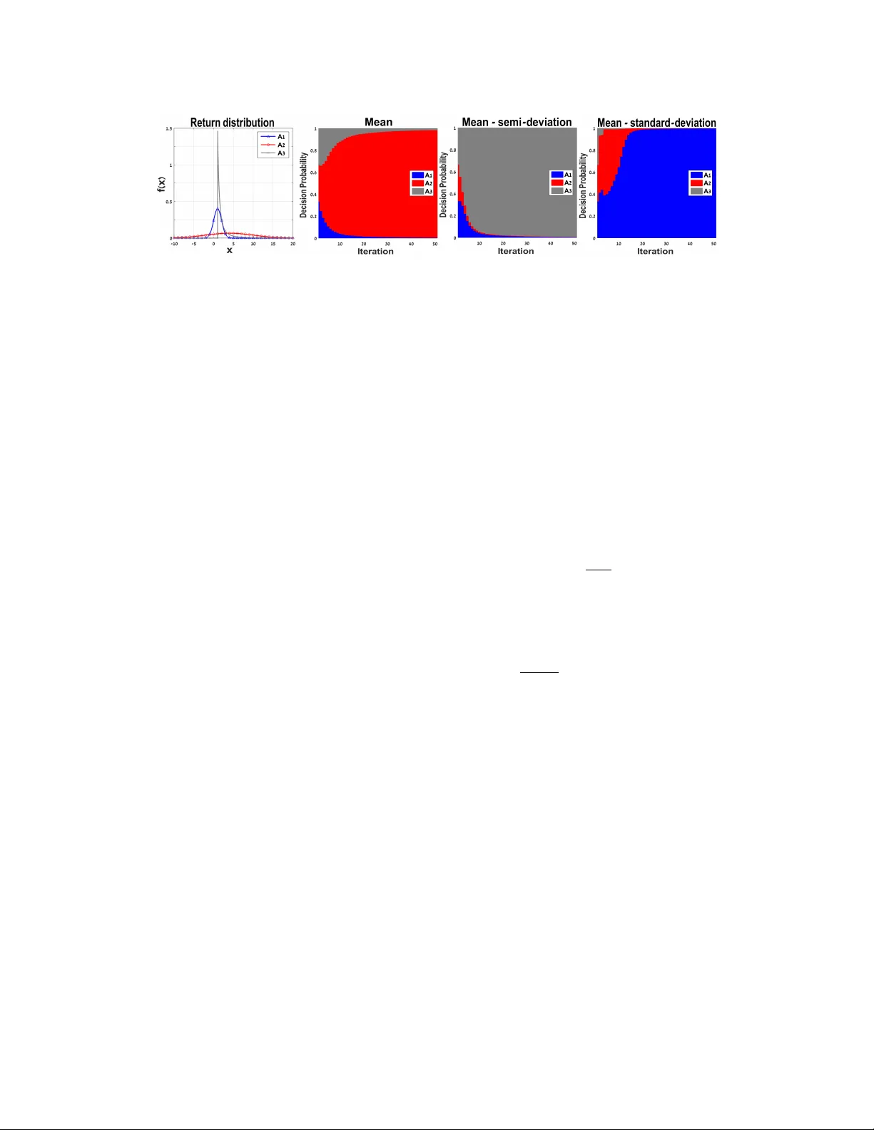
P olicy Gradient f or Coher ent Risk Measur es A viv T amar Electrical Engineering Department The T echnion - Israel Institute of T echnology avivt@tx.technion.ac.il Y inlam Chow Institute for Computational & Mathematical Engineering (ICME) Stanford Univ ersity ychow@stanford.edu Mohammad Ghavamzadeh Adobe Research & INRIA ghavamza@adobe.com Shie Mannor Electrical Engineering Department The T echnion - Israel Institute of T echnology shie@ee.technion.ac.il Abstract Sev eral authors hav e recently developed risk-sensiti ve polic y gradient methods that augment the standard expected cost minimization problem with a measure of variability in cost. These studies hav e focused on speciﬁc risk-measures, such as the variance or conditional value at risk (CV aR). In this work, we extend the pol- icy gradient method to the whole class of coherent risk measures, which is widely accepted in ﬁnance and operations research, among other ﬁelds. W e consider both static and time-consistent dynamic risk measures. For static risk measures, our approach is in the spirit of policy gr adient algorithms and combines a standard sampling approach with conv ex programming. For dynamic risk measures, our ap- proach is actor-critic style and in volv es explicit approximation of value function. Most importantly , our contribution presents a uniﬁed approach to risk-sensitiv e reinforcement learning that generalizes and extends pre vious results. 1 Introduction Risk-sensitiv e optimization considers problems in which the objecti ve inv olves a risk measure of the random cost, in contrast to the typical expected cost objectiv e. Such problems are important when the decision-maker wishes to manage the variability of the cost, in addition to its expected outcome, and are standard in various applications of ﬁnance and operations research. In reinforce- ment learning (RL) [33], risk-sensitiv e objectiv es have gained popularity as a means to regularize the variability of the total (discounted) cost/re ward in a Markov decision process (MDP). Many risk objecti ves have been in vestig ated in the literature and applied to RL, such as the cele- brated Marko witz mean-variance model [19], V alue-at-Risk (V aR) and Conditional V alue at Risk (CV aR) [22, 35, 26, 12, 10, 36]. The view taken in this paper is that the preference of one risk measure over another is pr oblem-dependent and depends on factors such as the cost distribution, sensitivity to rare ev ents, ease of estimation from data, and computational tractability of the op- timization problem. Ho we ver , the highly inﬂuential paper of Artzner et al. [2] identiﬁed a set of natural properties that are desirable for a risk measure to satisfy . Risk measures that satisfy these properties are termed coher ent and hav e obtained widespread acceptance in ﬁnancial applications, among others. W e focus on such coherent measures of risk in this work. For sequential decision problems, such as MDPs, another desirable property of a risk measure is time consistency . A time-consistent risk measure satisﬁes a “dynamic programming” style property: if a strategy is risk-optimal for an n -stage problem, then the component of the policy from the t -th 1 time until the end (where t < n ) is also risk-optimal (see principle of optimality in [5]). The recently proposed class of dynamic Mark ov coherent risk measures [30] satisﬁes both the coherence and time consistency properties. In this work, we present policy gradient algorithms for RL with a coherent risk objective. Our approach applies to the whole class of coherent risk measures, thereby generalizing and unifying previous approaches that hav e focused on individual risk measures. W e consider both static coherent risk of the total discounted return from an MDP and time-consistent dynamic Markov coherent risk. Our main contribution is formulating the risk-sensiti ve policy-gradient under the coherent-risk framew ork. More speciﬁcally , we provide: • A new formula for the gradient of static coherent risk that is con venient for approximation using sampling. • An algorithm for the gradient of general static coherent risk that in v olves sampling with con ve x programming and a corresponding consistency result. • A new polic y gradient theorem for Marko v coherent risk, relating the gradient to a suitable value function and a corresponding actor-critic algorithm. Sev eral pre vious results are special cases of the results presented here; our approach allo ws to re- deriv e them in greater generality and simplicity . Related W ork Risk-sensitiv e optimization in RL for speciﬁc risk functions has been studied re- cently by se veral authors. [8] studied exponential utility functions, [22], [35], [26] studied mean- variance models, [10], [36] studied CV aR in the static setting, and [25], [11] studied dynamic coher - ent risk for systems with linear dynamics. Our paper presents a general method for the whole class of coherent risk measures (both static and dynamic) and is not limited to a speciﬁc choice within that class, nor to particular system dynamics. Reference [24] showed that an MDP with a dynamic coherent risk objective is essentially a ro- bust MDP . The planning for large scale MDPs was considered in [37], using an approximation of the value function. For many problems, approximation in the polic y space is more suitable (see, e.g., [18]). Our sampling-based RL-style approach is suitable for approximations both in the policy and value function, and scales-up to large or continuous MDPs. W e do, ho wev er , make use of a technique of [37] in a part of our method. Optimization of coherent risk measures was thoroughly in vestigated by Ruszczynski and Shapiro [31] (see also [32]) for the stochastic programming case in which the policy parameters do not affect the distrib ution of the stochastic system (i.e., the MDP trajectory), but only the re ward function, and thus, this approach is not suitable for most RL problems. For the case of MDPs and dynamic risk, [30] proposed a dynamic programming approach. This approach does not scale-up to large MDPs, due to the “curse of dimensionality”. For further motiv ation of risk-sensitiv e policy gradient methods, we refer the reader to [22, 35, 26, 10, 36]. 2 Preliminaries Consider a probability space (Ω , F , P θ ) , where Ω is the set of outcomes (sample space), F is a σ -algebra ov er Ω representing the set of ev ents we are interested in, and P θ ∈ B , where B :=  ξ : R ω ∈ Ω ξ ( ω ) = 1 , ξ ≥ 0  is the set of probability distributions, is a probability measure over F parameterized by some tunable parameter θ ∈ R K . In the following, we suppress the notation of θ in θ -dependent quantities. T o ease the technical exposition, in this paper we restrict our attention to ﬁnite probability spaces, i.e., Ω has a ﬁnite number of elements. Our results can be e xtended to the L p -normed spaces without loss of generality , but the details are omitted for bre vity . Denote by Z the space of random variables Z : Ω 7→ ( −∞ , ∞ ) deﬁned over the probability space (Ω , F , P θ ) . In this paper , a random v ariable Z ∈ Z is interpreted as a cost, i.e., the smaller the realization of Z , the better . For Z , W ∈ Z , we denote by Z ≤ W the point-wise partial order , i.e., Z ( ω ) ≤ W ( ω ) for all ω ∈ Ω . W e denote by E ξ [ Z ] . = P ω ∈ Ω P θ ( ω ) ξ ( ω ) Z ( ω ) a ξ -weighted expectation of Z . 2 An MDP is a tuple M = ( X , A , C, P , γ , x 0 ) , where X and A are the state and action spaces; C ( x ) ∈ [ − C max , C max ] is a bounded, deterministic, and state-dependent cost; P ( ·| x, a ) is the tran- sition probability distribution; γ is a discount factor; and x 0 is the initial state. 1 Actions are chosen according to a θ -parameterized stationary Markov 2 policy µ θ ( ·| x ) . W e denote by x 0 , a 0 , . . . , x T , a T a trajectory of length T drawn by follo wing the policy µ θ in the MDP . 2.1 Coher ent Risk Measures A risk measur e is a function ρ : Z → R that maps an uncertain outcome Z to the extended real line R ∪ { + ∞ , −∞} , e.g., the expectation E [ Z ] or the conditional value-at-risk (CV aR) min ν ∈ R  ν + 1 α E  ( Z − ν ) +  . A risk measure is called coherent , if it satisﬁes the following conditions for all Z, W ∈ Z [2]: A1 Conv exity: ∀ λ ∈ [0 , 1] , ρ  λZ + (1 − λ ) W  ≤ λρ ( Z ) + (1 − λ ) ρ ( W ) ; A2 Monotonicity: if Z ≤ W , then ρ ( Z ) ≤ ρ ( W ) ; A3 Translation in variance: ∀ a ∈ R , ρ ( Z + a ) = ρ ( Z ) + a ; A4 Positive homogeneity: if λ ≥ 0 , then ρ ( λZ ) = λρ ( Z ) . Intuitiv ely , these condition ensure the “rationality” of single-period risk assessments: A1 ensures that div ersifying an in vestment will reduce its risk; A2 guarantees that an asset with a higher cost for every possible scenario is indeed riskier; A3, also known as ‘cash inv ariance’, means that the deterministic part of an in vestment portfolio does not contribute to its risk; the intuition behind A4 is that doubling a position in an asset doubles its risk. W e further refer the reader to [2] for a more detailed motiv ation of coherent risk. The following representation theorem [32] shows an important property of coherent risk measures that is fundamental to our gradient-based approach. Theorem 2.1. A risk measure ρ : Z → R is coher ent if and only if ther e exists a conve x bounded and closed set U ⊂ B such that 3 ρ ( Z ) = max ξ : ξ P θ ∈U ( P θ ) E ξ [ Z ] . (1) The result essentially states that any coherent risk measure is an expectation w .r .t. a w orst-case den- sity function ξ P θ , chosen adversarially from a suitable set of test density functions U ( P θ ) , referred to as risk en velope . Moreover , it means that any coherent risk measure is uniquely r epresented by its risk env elope. Thus, in the sequel, we shall interchangeably refer to coherent risk-measures either by their explicit functional representation, or by their corresponding risk-en velope. In this paper, we assume that the risk en velop U ( P θ ) is given in a canonical conv ex programming formulation, and satisﬁes the following conditions. Assumption 2.2 (The General Form of Risk En velope) . F or each given policy parameter θ ∈ R K , the risk en velope U of a coher ent risk measur e can be written as U ( P θ ) =  ξ P θ : g e ( ξ , P θ ) = 0 , ∀ e ∈ E , f i ( ξ , P θ ) ≤ 0 , ∀ i ∈ I , X ω ∈ Ω ξ ( ω ) P θ ( ω ) = 1 , ξ ( ω ) ≥ 0  , (2) wher e each constraint g e ( ξ , P θ ) is an af ﬁne function in ξ , each constraint f i ( ξ , P θ ) is a con vex function in ξ , and there exists a strictly feasible point ξ . E and I her e denote the sets of equality and inequality constraints, r espectively . Furthermore , for any given ξ ∈ B , f i ( ξ , p ) and g e ( ξ , p ) ar e twice differ entiable in p , and there e xists a M > 0 suc h that max  max i ∈I     d f i ( ξ , p ) dp ( ω )     , max e ∈E     dg e ( ξ , p ) dp ( ω )      ≤ M , ∀ ω ∈ Ω . 1 Our results may easily be e xtended to random costs, state-action dependent costs, and random initial states. 2 For the dynamic Markov risk we study , an optimal policy is stationary Markov , while this is not necessarily the case for the static risk. Our results can be extended to history-dependent policies or stationary Markov policies on a state space augmented with the accumulated cost. The latter has sho wn to be suf ﬁcient for optimizing the CV aR risk [4]. 3 When we study risk in MDPs, the risk en velop U ( P θ ) in Eq. 1 also depends on the state x . 3 Assumption 2.2 implies that the risk en velope U ( P θ ) is known in an explicit form. From Theorem 6.6 of [32], in the case of a ﬁnite probability space, ρ is a coherent risk if and only if U ( P θ ) is a con ve x and compact set. This justiﬁes the afﬁne assumption of g e and the con ve x assumption of f i . Moreov er , the additional assumption on the smoothness of the constraints holds for many popular coherent risk measures, such as the CV aR, the mean-semi-deviation, and spectral risk measures [1]. 2.2 Dynamic Risk Measures The risk measures deﬁned abov e do not take into account any temporal structure that the random variable might have, such as when it is associated with the return of a trajectory in the case of MDPs. In this sense, such risk measures are called static . Dynamic risk measures, on the other hand, explicitly take into account the temporal nature of the stochastic outcome. A primary motiv ation for considering such measures is the issue of time consistency , usually deﬁned as follows [30]: if a certain outcome is considered less risky in all states of the world at stage t + 1 , then it should also be considered less risky at stage t . Example 2.1 in [16] shows the importance of time consistency in the ev aluation of risk in a dynamic setting. It illustrates that for multi-period decision-making, optimizing a static measure can lead to “time-inconsistent” behavior . Similar paradoxical results could be obtained with other risk metrics; we refer the readers to [30] and [16] for further insights. Markov Coherent Risk Measures. Markov risk measures were introduced in [30] and are a useful class of dynamic time-consistent risk measures that are particularly important for our study of risk in MDPs. For a T -length horizon and MDP M , the Markov coherent risk measure ρ T ( M ) is ρ T ( M ) = C ( x 0 ) + γ ρ C ( x 1 ) + . . . + γ ρ  C ( x T − 1 ) + γ ρ  C ( x T )   ! , (3) where ρ is a static coherent risk measure that satisﬁes Assumption 2.2 and x 0 , . . . , x T is a trajectory drawn from the MDP M under policy µ θ . It is important to note that in (3), each static coherent risk ρ at state x ∈ X is induced by the transition probability P θ ( ·| x ) = P a ∈A P ( x 0 | x, a ) µ θ ( a | x ) . W e also deﬁne ρ ∞ ( M ) . = lim T →∞ ρ T ( M ) , which is well-deﬁned since γ < 1 and the cost is bounded. W e further assume that ρ in (3) is a Marko v risk measure, i.e., the ev aluation of each static coherent risk measure ρ is not allowed to depend on the whole past. 3 Problem F ormulation In this paper , we are interested in solving two risk-sensitiv e optimization problems. Gi ven a random variable Z and a static coherent risk measure ρ as deﬁned in Section 2, the static risk problem (SRP) is giv en by min θ ρ ( Z ) . (4) For example, in an RL setting, Z may correspond to the cumulativ e discounted cost Z = C ( x 0 ) + γ C ( x 1 ) + · · · + γ T C ( x T ) of a trajectory induced by an MDP with a policy parameterized by θ . For an MDP M and a dynamic Markov coherent risk measure ρ T as deﬁned by Eq. 3, the dynamic risk problem (DRP) is giv en by min θ ρ ∞ ( M ) . (5) Except for very limited cases, there is no reason to hope that neither the SRP in (4) nor the DRP in (5) should be tractable problems, since the dependence of the risk measure on θ may be complex and non-con vex. In this work, we aim towards a more modest goal and search for a locally optimal θ . Thus, the main problem that we are trying to solve in this paper is how to calculate the gradients of the SRP’ s and DRP’ s objecti ve functions ∇ θ ρ ( Z ) and ∇ θ ρ ∞ ( M ) . W e are interested in non-trivial cases in which the gradients cannot be calculated analytically . In the static case, this would correspond to a non-trivial dependence of Z on θ . For dynamic risk, we also consider cases where the state space is too large for a tractable computation. Our approach for dealing with such difﬁcult cases is through sampling. W e assume that in the static case, we may obtain i.i.d. samples of the random variable Z . For the dynamic case, we assume that for each state and action ( x, a ) of the MDP , we may obtain i.i.d. samples of the next state x 0 ∼ P ( ·| x, a ) . W e show that sampling may indeed be used in both cases to de vise suitable estimators for the gradients. 4 T o ﬁnally solve the SRP and DRP problems, a gradient estimate may be plugged into a standard stochastic gradient descent (SGD) algorithm for learning a locally optimal solution to (4) and (5). From the structure of the dynamic risk in Eq. 3, one may think that a gradient estimator for ρ ( Z ) may help us to estimate the gradient ∇ θ ρ ∞ ( M ) . Indeed, we follow this idea and begin with estimating the gradient in the static risk case. 4 Gradient Formula for Static Risk In this section, we consider a static coherent risk measure ρ ( Z ) and propose sampling-based es- timators for ∇ θ ρ ( Z ) . W e make the following assumption on the policy parametrization, which is standard in the policy gradient literature [18]. Assumption 4.1. The lik elihood ratio ∇ θ log P ( ω ) is well-deﬁned and bounded for all ω ∈ Ω . Moreov er , our approach implicitly assumes that gi ven some ω ∈ Ω , ∇ θ log P ( ω ) may be easily calculated. This is also a standard requirement for policy gradient algorithms [18] and is satisﬁed in v arious applications such as queueing systems, in ventory management, and ﬁnancial engineering (see, e.g., the surve y by Fu [14]). Using Theorem 2.1 and Assumption 2.2, for each θ , we have that ρ ( Z ) is the solution to the con- ve x optimization problem (1) (for that value of θ ). The Lagrangian function of (1), denoted by L θ ( ξ , λ P , λ E , λ I ) , may be written as L θ ( ξ , λ P , λ E , λ I ) = X ω ∈ Ω ξ ( ω ) P θ ( ω ) Z ( ω ) − λ P X ω ∈ Ω ξ ( ω ) P θ ( ω ) − 1 ! − X e ∈E λ E ( e ) g e ( ξ ,P θ ) − X i ∈I λ I ( i ) f i ( ξ ,P θ ) . (6) The con ve xity of (1) and its strict feasibility due to Assumption 2.2 implies that L θ ( ξ , λ P , λ E , λ I ) has a non-empty set of saddle points S . The next theorem presents a formula for the gradient ∇ θ ρ ( Z ) . As we shall subsequently show , this formula is particularly con venient for devising sam- pling based estimators for ∇ θ ρ ( Z ) . Theorem 4.2. Let Assumptions 2.2 and 4.1 hold. F or any saddle point ( ξ ∗ θ , λ ∗ , P θ , λ ∗ , E θ , λ ∗ , I θ ) ∈ S of (6) , we have ∇ θ ρ ( Z ) = E ξ ∗ θ h ∇ θ log P ( ω )( Z − λ ∗ , P θ ) i − X e ∈E λ ∗ , E θ ( e ) ∇ θ g e ( ξ ∗ θ ; P θ ) − X i ∈I λ ∗ , I θ ( i ) ∇ θ f i ( ξ ∗ θ ; P θ ) . The proof of this theorem, giv en in the supplementary material, in volves an application of the En ve- lope theorem [21] and a standard ‘likelihood-ratio’ trick. W e now demonstrate the utility of Theorem 4.2 with several examples in which we show that it generalizes previously known results, and also enables deriving ne w useful gradient formulas. 4.1 Example 1: CV aR The CV aR at level α ∈ [0 , 1] of a random variable Z , denoted by ρ CV aR ( Z ; α ) , is a very popular coherent risk measure [28], deﬁned as ρ CV aR ( Z ; α ) . = inf t ∈ R  t + α − 1 E [( Z − t ) + ]  . When Z is continuous, ρ CV aR ( Z ; α ) is well-known to be the mean of the α -tail distribution of Z , E [ Z | Z > q α ] , where q α is a (1 − α ) -quantile of Z . Thus, selecting a small α makes CV aR partic- ularly sensitiv e to rare, b ut very high costs. The risk en velope for CV aR is known to be [32] U =  ξ P θ : ξ ( ω ) ∈ [0 , α − 1 ] , P ω ∈ Ω ξ ( ω ) P θ ( ω ) = 1  . Furthermore, [32] show that the saddle points of (6) satisfy ξ ∗ θ ( ω ) = α − 1 when Z ( ω ) > λ ∗ , P θ , and ξ ∗ θ ( ω ) = 0 when Z ( ω ) < λ ∗ , P θ , where λ ∗ , P θ is any (1 − α ) - quantile of Z . Plugging this result into Theorem 4.2, we can easily sho w that ∇ θ ρ CV aR ( Z ; α ) = E [ ∇ θ log P ( ω )( Z − q α ) | Z ( ω ) > q α ] . This formula was recently proved in [36] for the case of continuous distributions by an explicit calculation of the conditional expectation, and under several additional smoothness assumptions. Here we show that it holds regardless of these assumptions and in the discrete case as well. Our proof is also considerably simpler . 5 4.2 Example 2: Mean-Semideviation The semi-deviation of a random variable Z is deﬁned as SD [ Z ] . =  E  ( Z − E [ Z ]) 2 +  1 / 2 . The semi-deviation captures the v ariation of the cost only above its mean , and is an appealing alternati ve to the standard de viation, which does not distinguish between the v ariability of upside and downside deviations. For some α ∈ [0 , 1] , the mean-semideviation risk measure is deﬁned as ρ MSD ( Z ; α ) . = E [ Z ] + α SD [ Z ] , and is a coherent risk measure [32]. W e hav e the follo wing result: Proposition 4.3. Under Assumption 4.1, with ∇ θ E [ Z ] = E [ ∇ θ log P ( ω ) Z ] , we have ∇ θ ρ MSD ( Z ; α ) = ∇ θ E [ Z ] + α E [( Z − E [ Z ]) + ( ∇ θ log P ( ω )( Z − E [ Z ]) − ∇ θ E [ Z ])] SD ( Z ) . This proposition can be used to devise a sampling based estimator for ∇ θ ρ MSD ( Z ; α ) by replacing all the expectations with sample av erages. The algorithm along with the proof of the proposition are in the supplementary material. In Section 6 we pro vide a numerical illustration of optimization with a mean-semideviation objecti ve. 4.3 General Gradient Estimation Algorithm In the two previous examples, we obtained a gradient formula by analytically calculating the La- grangian saddle point (6) and plugging it into the formula of Theorem 4.2. W e no w consider a general coherent risk ρ ( Z ) for which, in contrast to the CV aR and mean-semideviation cases, the Lagrangian saddle-point is not known analytically . W e only assume that we know the structur e of the risk-en velope as given by (2). W e show that in this case, ∇ θ ρ ( Z ) may be estimated using a sample averag e appr oximation (SAA; [32]) of the formula in Theorem 4.2. Assume that we are given N i.i.d. samples ω i ∼ P θ , i = 1 , . . . , N , and let P θ ; N ( ω ) . = 1 N P N i =1 I { ω i = ω } denote the corresponding empirical distribution. Also, let the sample risk en- velope U ( P θ ; N ) be deﬁned according to Eq. 2 with P θ replaced by P θ ; N . Consider the following SAA version of the optimization in Eq. 1: ρ N ( Z ) = max ξ : ξ P θ ; N ∈U ( P θ ; N ) X i ∈ 1 ,...,N P θ ; N ( ω i ) ξ ( ω i ) Z ( ω i ) . (7) Note that (7) deﬁnes a con ve x optimization problem with O ( N ) variables and constraints. In the following, we assume that a solution to (7) may be computed ef ﬁciently using standard con- ve x programming tools such as interior point methods [9]. Let ξ ∗ θ ; N denote a solution to (7) and λ ∗ , P θ ; N , λ ∗ , E θ ; N , λ ∗ , I θ ; N denote the corresponding KKT multipliers, which can be obtained from the con- ve x programming algorithm [9]. W e propose the following estimator for the gradient-based on Theorem 4.2: ∇ θ ; N ρ ( Z ) = N X i =1 P θ ; N ( ω i ) ξ ∗ θ ; N ( ω i ) ∇ θ log P ( ω i )( Z ( ω i ) − λ ∗ , P θ ; N ) (8) − X e ∈E λ ∗ , E θ ; N ( e ) ∇ θ g e ( ξ ∗ θ ; N ; P θ ; N ) − X i ∈I λ ∗ , I θ ; N ( i ) ∇ θ f i ( ξ ∗ θ ; N ; P θ ; N ) . Thus, our gradient estimation algorithm is a two-step procedure in v olving both sampling and con vex pr ogramming . In the follo wing, we show that under some conditions on the set U ( P θ ) , ∇ θ ; N ρ ( Z ) is a consistent estimator of ∇ θ ρ ( Z ) . The proof has been reported in the supplementary material. Proposition 4.4. Let Assumptions 2.2 and 4.1 hold. Suppose ther e exists a compact set C = C ξ × C λ such that: (I) The set of Lagr angian saddle points S ⊂ C is non-empty and bounded. (II) The functions f e ( ξ , P θ ) for all e ∈ E and f i ( ξ , P θ ) for all i ∈ I ar e ﬁnite-valued and continuous (in ξ ) on C ξ . (III) F or N lar ge enough, the set S N is non-empty and S N ⊂ C w .p. 1. Further assume that: (IV) If ξ N P θ ; N ∈ U ( P θ ; N ) and ξ N con ver ges w .p. 1 to a point ξ , then ξ P θ ∈ U ( P θ ) . W e then have that lim N →∞ ρ N ( Z ) = ρ ( Z ) and lim N →∞ ∇ θ ; N ρ ( Z ) = ∇ θ ρ ( Z ) w .p. 1. The set of assumptions for Proposition 4.4 is lar ge, but rather mild. Note that (I) is implied by the Slater condition of Assumption 2.2. For satisfying (III), we need that the risk be well-deﬁned for e very empirical distrib ution, which is a natural requirement. Since P θ ; N always con ver ges to P θ uniformly on Ω , (IV) essentially requires smoothness of the constraints. W e remark that in particular , 6 constraints (I) to (IV) are satisﬁed for the popular CV aR, mean-semideviation, and spectral risk measures. T o summarize this section, we hav e seen that by exploiting the special structure of coherent risk measures in Theorem 2.1 and by the en velope-theorem style result of Theorem 4.2, we were able to deriv e sampling-based, likelihood-ratio style algorithms for estimating the policy gradient ∇ θ ρ ( Z ) of coherent static risk measures. The gradient estimation algorithms dev eloped here for static risk measures will be used as a sub-routine in our subsequent treatment of dynamic risk measures. 5 Gradient Formula for Dynamic Risk In this section, we deriv e a ne w formula for the gradient of the Markov coherent dynamic risk mea- sure, ∇ θ ρ ∞ ( M ) . Our approach is based on combining the static gradient formula of Theorem 4.2, with a dynamic-programming decomposition of ρ ∞ ( M ) . The risk-sensitiv e value-function for an MDP M under the polic y θ is deﬁned as V θ ( x ) = ρ ∞ ( M| x 0 = x ) , where with a slight abuse of notation, ρ ∞ ( M| x 0 = x ) denotes the Marko v- coherent dynamic risk in (3) when the initial state x 0 is x . It is sho wn in [30] that due to the structure of the Markov dynamic risk ρ ∞ ( M ) , the value function is the unique solution to the risk-sensitive Bellman equation V θ ( x ) = C ( x ) + γ max ξP θ ( ·| x ) ∈U ( x,P θ ( ·| x )) E ξ [ V θ ( x 0 )] , (9) where the expectation is taken over the next state transition. Note that by deﬁnition, we have ρ ∞ ( M ) = V θ ( x 0 ) , and thus, ∇ θ ρ ∞ ( M ) = ∇ θ V θ ( x 0 ) . W e no w dev elop a formula for ∇ θ V θ ( x ) ; this formula extends the well-known “polic y gradient theorem” [34, 17], developed for the expected return, to Markov-coherent dynamic risk measures. W e make a standard assumption, analogous to Assumption 4.1 of the static case. Assumption 5.1. The likelihood ratio ∇ θ log µ θ ( a | x ) is well-deﬁned and bounded for all x ∈ X and a ∈ A . For each state x ∈ X , let ( ξ ∗ θ,x , λ ∗ , P θ,x , λ ∗ , E θ,x , λ ∗ , I θ,x ) denote a saddle point of (6), corresponding to the state x , with P θ ( ·| x ) replacing P θ in (6) and V θ replacing Z . The next theorem presents a formula for ∇ θ V θ ( x ) ; the proof is in the supplementary material. Theorem 5.2. Under Assumptions 2.2 and 5.1, we have ∇ V θ ( x ) = E ξ ∗ θ " ∞ X t =0 γ t ∇ θ log µ θ ( a t | x t ) h θ ( x t , a t )      x 0 = x # , wher e E ξ ∗ θ [ · ] denotes the expectation w .r .t. trajectories generated by the Markov chain with transition pr obabilities P θ ( ·| x ) ξ ∗ θ,x ( · ) , and the stage-wise cost function h θ ( x, a ) is deﬁned as h θ ( x, a ) = C ( x )+ X x 0 ∈X P ( x 0 | x, a ) ξ ∗ θ,x ( x 0 ) " γ V θ ( x 0 ) − λ ∗ , P θ,x − X i ∈I λ ∗ , I θ,x ( i ) d f i ( ξ ∗ θ,x , p ) dp ( x 0 ) − X e ∈E λ ∗ , E θ,x ( e ) dg e ( ξ ∗ θ,x , p ) dp ( x 0 ) # . Theorem 5.2 may be used to develop an actor-critic style [34, 17] sampling-based algorithm for solving the DRP problem (5), composed of two interlea ved procedures: Critic: For a gi ven polic y θ , calculate the risk-sensiti ve v alue function V θ , and Actor: Using the critic’ s V θ and Theorem 5.2, estimate ∇ θ ρ ∞ ( M ) and update θ . Space limitation restricts us from specifying the full details of our actor-critic algorithm and its analysis. In the following, we highlight only the key ideas and results. For the full details, we refer the reader to the full paper version, pro vided in the supplementary material. For the critic, the main challenge is calculating the value function when the state space X is large and dynamic programming cannot be applied due to the ‘curse of dimensionality’. T o ov ercome this, we exploit the fact that V θ is equiv alent to the value function in a robust MDP [24] and modify a recent algorithm in [37] to estimate it using function approximation. For the actor , the main challenge is that in order to estimate the gradient using Thm. 5.2, we need to sample from an MDP with ξ ∗ θ -weighted transitions. Also, h θ ( x, a ) in volv es an expectation for each 7 Figure 1: Numerical illustration - selection between 3 assets. A: Probability density of asset return. B,C,D: Bar plots of the probability of selecting each asset vs. training iterations, for policies π 1 , π 2 , and π 3 , respectiv ely . At each iteration, 10,000 samples were used for gradient estimation. s and a . Therefore, we propose a two-phase sampling pr ocedur e to estimate ∇ V θ in which we ﬁrst use the critic’ s estimate of V θ to derive ξ ∗ θ , and sample a trajectory from an MDP with ξ ∗ θ -weighted transitions. For each state in the trajectory , we then sample several ne xt states to estimate h θ ( x, a ) . The con vergence analysis of the actor-critic algorithm and the gradient error incurred from function approximation of V θ are reported in the supplementary material. 6 Numerical Illustration In this section, we illustrate our approach with a numerical example. The purpose of this illustration is to emphasize the importance of ﬂexibility in designing risk criteria for selecting an appr opriate risk-measure – such that suits both the user’ s risk preference and the problem-speciﬁc properties. W e consider a trading agent that can inv est in one of three assets (see Figure 1 for their distrib utions). The returns of the ﬁrst two assets, A 1 and A 2 , are normally distributed: A 1 ∼ N (1 , 1) and A 2 ∼ N (4 , 6) . The return of the third asset A 3 has a Pareto distribution: f ( z ) = α z α +1 ∀ z > 1 , with α = 1 . 5 . The mean of the return from A 3 is 3 and its variance is inﬁnite; such heavy-tailed distributions are widely used in ﬁnancial modeling [27]. The agent selects an action randomly , with probability P ( A i ) ∝ exp( θ i ) , where θ ∈ R 3 is the policy parameter . W e trained three different policies π 1 , π 2 , and π 3 . Policy π 1 is risk-neutral, i.e., max θ E [ Z ] , and it was trained using standard policy gradient [18]. Policy π 2 is risk-av erse and had a mean-semide viation objectiv e max θ E [ Z ] − SD [ Z ] , and was trained using the algorithm in Section 4. Policy π 3 is also risk-av erse, with a mean-standard- deviation objectiv e, as proposed in [35, 26], max θ E [ Z ] − p V ar [ Z ] , and was trained using the algorithm of [35]. For each of these policies, Figure 1 shows the probability of selecting each asset vs. training iterations. Although A 2 has the highest mean return, the risk-av erse policy π 2 chooses A 3 , since it has a lower do wnside, as expected. Ho we ver , because of the heavy upper-tail of A 3 , policy π 3 opted to choose A 1 instead. This is counter -intuitiv e as a rational in vestor should not avert high returns. In fact, in this case A 3 stochastically dominates A 1 [15]. 7 Conclusion W e presented algorithms for estimating the gradient of both static and dynamic coherent risk mea- sures using two new policy gradient style formulas that combine sampling with conv ex program- ming. Thereby , our approach e xtends risk-sensitiv e RL to the whole class of coherent risk measures, and generalizes sev eral recent studies that focused on speciﬁc risk measures. On the technical side, an important future direction is to improv e the conv ergence rate of gradient estimates using importance sampling methods. This is especially important for risk criteria that are sensitiv e to rare e vents, such as the CV aR [3]. From a more conceptual point of view , the coherent-risk framework explored in this work provides the decision maker with ﬂexibility in designing risk preference. As our numerical example shows, such ﬂexibility is important for selecting appropriate pr oblem-speciﬁc risk measures for managing the cost variability . Howe ver , we believ e that our approach has much more potential than that. In almost e very real-world application, uncertainty emanates from stochastic dynamics, but also, and perhaps more importantly , from modeling errors (model uncertainty). A prudent policy should 8 protect against both types of uncertainties. The representation duality of coherent-risk (Theorem 2.1), naturally relates the risk to model uncertainty . In [24], a similar connection was made between model-uncertainty in MDPs and dynamic Markov coherent risk. W e believ e that by carefully shap- ing the risk-criterion, the decision maker may be able to take uncertainty into account in a br oad sense. Designing a principled procedure for such risk-shaping is not tri vial, and is beyond the scope of this paper . Ho wev er , we believ e that there is much potential to risk shaping as it may be the key for handling model misspeciﬁcation in dynamic decision making. References [1] C. Acerbi. Spectral measures of risk: a coherent representation of subjective risk av ersion. J ournal of Banking & F inance , 26(7):1505–1518, 2002. [2] P . Artzner , F . Delbaen, J. Eber, and D. Heath. Coherent measures of risk. Mathematical ﬁnance , 9(3):203– 228, 1999. [3] O. Bardou, N. Frikha, and G. Pag ` es. Computing VaR and CVaR using stochastic approximation and adaptiv e unconstrained importance sampling. Monte Carlo Methods and Applications , 15(3):173–210, 2009. [4] N. B ¨ auerle and J. Ott. Marko v decision processes with av erage-value-at-risk criteria. Mathematical Methods of Operations Resear ch , 74(3):361–379, 2011. [5] D. Bertsekas. Dynamic Pr ogramming and Optimal Contr ol . Athena Scientiﬁc, 4th edition, 2012. [6] D. Bertsekas and J. Tsitsiklis. Neur o-Dynamic Pr ogr amming . Athena Scientiﬁc, 1996. [7] S. Bhatnagar , R. Sutton, M. Ghav amzadeh, and M. Lee. Natural actor-critic algorithms. Automatica , 45(11):2471–2482, 2009. [8] V . Borkar . A sensitivity formula for risk-sensiti ve cost and the actor –critic algorithm. Systems & Contr ol Letters , 44(5):339–346, 2001. [9] S. Boyd and L. V andenberghe. Conve x optimization . Cambridge university press, 2009. [10] Y . Chow and M. Gha vamzadeh. Algorithms for CV aR optimization in MDPs. In NIPS 27 , 2014. [11] Y . Cho w and M. Pav one. A unifying frame work for time-consistent, risk-av erse model predicti ve control: theory and algorithms. In American Control Confer ence , 2014. [12] E. Delage and S. Mannor . Percentile optimization for Markov decision processes with parameter uncer- tainty . Operations Resear ch , 58(1):203213, 2010. [13] A. Fiacco. Intr oduction to sensitivity and stability analysis in nonlinear pr ogr amming . Else vier , 1983. [14] M. Fu. Gradient estimation. In Simulation , volume 13 of Handbooks in Operations Researc h and Man- agement Science , pages 575 – 616. Else vier , 2006. [15] J. Hadar and W . R. Russell. Rules for ordering uncertain prospects. The American Economic Review , pages 25–34, 1969. [16] D. Iancu, M. Petrik, and D. Subramanian. T ight approximations of dynamic risk measures. arXiv:1106.6102 , 2011. [17] V . K onda and J. Tsitsiklis. Actor-critic algorithms. In NIPS , 2000. [18] P . Marbach and J. Tsitsiklis. Simulation-based optimization of Marko v re ward processes. IEEE T ransac- tions on Automatic Contr ol , 46(2):191–209, 1998. [19] H. Markowitz. P ortfolio Selection: Efﬁcient Diversiﬁcation of In vestment . John W iley and Sons, 1959. [20] F . Meng and H. Xu. A regularized sample average approximation method for stochastic mathematical programs with nonsmooth equality constraints. SIAM Journal on Optimization , 17(3):891–919, 2006. [21] P . Milgrom and I. Segal. En velope theorems for arbitrary choice sets. Econometrica , 70(2):583–601, 2002. [22] J. Moody and M. Saffell. Learning to trade via direct reinforcement. Neural Networks, IEEE T ransactions on , 12(4):875–889, 2001. [23] A. Nilim and L. El Ghaoui. Robust control of Marko v decision processes with uncertain transition matri- ces. Operations Resear ch , 53(5):780–798, 2005. [24] T . Osogami. Robustness and risk-sensiti vity in Markov decision processes. In NIPS , 2012. [25] M. Petrik and D. Subramanian. An approximate solution method for large risk-a verse Markov decision processes. In UAI , 2012. [26] L. Prashanth and M. Ghavamzadeh. Actor-critic algorithms for risk-sensiti ve MDPs. In NIPS 26 , 2013. 9 [27] S. Rachev and S. Mittnik. Stable P aretian models in ﬁnance . John W illey & Sons, Ne w Y ork, 2000. [28] R. Rockafellar and S. Uryase v . Optimization of conditional v alue-at-risk. Journal of risk , 2:21–42, 2000. [29] R. Rockafellar, R. W ets, and M. W ets. V ariational analysis , volume 317. Springer, 1998. [30] A. Ruszczy ´ nski. Risk-averse dynamic programming for Markov decision processes. Mathematical Pro- gramming , 125(2):235–261, 2010. [31] A. Ruszczy ´ nski and A. Shapiro. Optimization of con ve x risk functions. Math. OR , 31(3):433–452, 2006. [32] A. Shapiro, D. Dentchev a, and A. Ruszczy ´ nski. Lectur es on Stochastic Pr ogr amming , chapter 6, pages 253–332. SIAM, 2009. [33] R. Sutton and A. Barto. Reinfor cement learning: An intr oduction . Cambridge Univ Press, 1998. [34] R. Sutton, D. McAllester, S. Singh, and Y . Mansour . Policy gradient methods for reinforcement learning with function approximation. In NIPS 13 , 2000. [35] A. T amar , D. Di Castro, and S. Mannor . Policy gradients with v ariance related risk criteria. In Interna- tional Confer ence on Machine Learning , 2012. [36] A. T amar, Y . Glassner, and S. Mannor . Optimizing the CV aR via sampling. In AAAI , 2015. [37] A. T amar, S. Mannor , and H. Xu. Scaling up robust MDPs using function approximation. In International Confer ence on Machine Learning , 2014. 10 A Proof of Theor em 4.2 First note from Assumption 2.2 that (i) Slater’ s condition holds in the primal optimization problem (1), (ii) L θ ( ξ , λ P , λ E , λ I ) is con ve x in ξ and concav e in ( λ P , λ E , λ I ) . Thus by the duality result in conv ex optimization [9], the abov e conditions imply strong duality and we hav e ρ ( Z ) = max ξ ≥ 0 min λ P ,λ I ≥ 0 ,λ E L θ ( ξ , λ P , λ E , λ I ) = min λ P ,λ I ≥ 0 ,λ E max ξ ≥ 0 L θ ( ξ , λ P , λ E , λ I ) . From Assumption 2.2, one can also see that the family of functions { L θ ( ξ , λ P , λ E , λ I ) } ( ξ,λ P ,λ E ,λ I ) ∈ R | Ω | × R × R |E | × R |I | is equi-differentiable in θ , L θ ( ξ , λ P , λ E , λ I ) is Lipschitz, as a result, an absolutely continuous function in θ , and thus, ∇ θ L θ ( ξ , λ P , λ E , λ I ) is continuous and bounded at each ( ξ , λ P , λ E , λ I ) . Then for e very selection of saddle point ( ξ ∗ θ , λ ∗ , P θ , λ ∗ , E θ , λ ∗ , I θ ) ∈ S of (6), using the En velop theorem for saddle-point problems (see Theorem 4 of [21]), we hav e ∇ θ max ξ ≥ 0 min λ P ,λ I ≥ 0 ,λ E L θ ( ξ , λ P , λ E , λ I ) = ∇ θ L θ ( ξ , λ P , λ E , λ I ) | ( ξ ∗ θ ,λ ∗ , P θ ,λ ∗ , E θ ,λ ∗ , I θ ) . (10) The result follows by writing the gradient in (10) e xplicitly , and using the likelihood-ratio trick: X ω ∈ Ω ξ ( ω ) ∇ θ P θ ( ω ) Z ( ω ) − λ P X ω ∈ Ω ξ ( ω ) ∇ θ P θ ( ω ) = X ω ∈ Ω ξ ( ω ) P ( ω ) ∇ θ log P ( ω )  Z ( ω ) − λ P  , where the last equality is justiﬁed by Assumption 4.1. B Gradient Results for Static Mean-Semideviation In this section we consider the mean-semideviation risk measure, deﬁned as follo ws: ρ MSD ( Z ) = E [ Z ] + c  E  ( Z − E [ Z ]) 2 +  1 / 2 , (11) Follo wing the deriv ation in [32], note that  E  | Z | 2  1 / 2 = k Z k 2 , where k · k 2 denotes the L 2 norm of the space L 2 (Ω , F , P θ ) . The norm may also be written as: k Z k 2 = sup k ξ k 2 ≤ 1 h ξ , Z i , and hence  E  ( Z − E [ Z ]) 2 +  1 / 2 = sup k ξ k 2 ≤ 1 h ξ , ( Z − E [ Z ]) + i = sup k ξ k 2 ≤ 1 ,ξ ≥ 0 h ξ , Z − E [ Z ] i = sup k ξ k 2 ≤ 1 ,ξ ≥ 0 h ξ − E [ ξ ] , Z i . It follows that Eq. (1) holds with U = { ξ 0 ∈ Z ∗ : ξ 0 = 1 + cξ − c E [ ξ ] , k ξ k q ≤ 1 , ξ ≥ 0 } . For this case it will be more con venient to write Eq. (1) in the following form ρ MSD ( Z ) = sup k ξ k q ≤ 1 ,ξ ≥ 0 h 1 + cξ − c E [ ξ ] , Z i . (12) Let ¯ ξ denote an optimal solution for (12). In [32] it is sho wn that ¯ ξ is a contact point of ( Z − E [ Z ]) + , that is ¯ ξ ∈ arg max {h ξ , ( Z − E [ Z ]) + i : k ξ k 2 ≤ 1 } , and we hav e that ¯ ξ = ( Z − E [ Z ]) + k ( Z − E [ Z ]) + k 2 = ( Z − E [ Z ]) + SD ( Z ) . (13) Note that ¯ ξ is not necessarily a probability distribution, but for c ∈ [0 , 1] , it can be shown [32] that 1 + c ¯ ξ − c E  ¯ ξ  always is. In the following we show that ¯ ξ may be used to write the gradient ∇ θ ρ MSD ( Z ) as an expectation, which will lead to a sampling algorithm for the gradient. 11 Proposition B.1. Under Assumption 4.1, we have that ∇ θ ρ MSD ( Z ) = ∇ θ E [ Z ] + c SD ( Z ) E [( Z − E [ Z ]) + ( ∇ θ log P ( ω )( Z − E [ Z ]) − ∇ θ E [ Z ])] , and, accor ding to the standar d likelihood-r atio method, ∇ θ E [ Z ] = E [ ∇ θ log P ( ω ) Z ] . Pr oof. Note that in Eq. (12) the constraints do not depend on θ . Therefore, using the en velope theorem we obtain that ∇ θ ρ ( Z ) = ∇ θ h 1 + c ¯ ξ − c E  ¯ ξ  , Z i = ∇ θ h 1 , Z i + c ∇ θ h ¯ ξ , Z i − c ∇ θ h E  ¯ ξ  , Z i . (14) W e now write each of the terms in Eq. (14) as an expectation. W e start with the following standard likelihood-ratio result: ∇ θ h 1 , Z i = ∇ θ E [ Z ] = E [ ∇ θ log P ( ω ) Z ] . Also, we hav e that h E  ¯ ξ  , Z i = E  ¯ ξ  E [ Z ] , therefore, by the deriv ative of a product rule: ∇ θ h E  ¯ ξ  , Z i = ∇ θ E  ¯ ξ  E [ Z ] + E  ¯ ξ  ∇ θ E [ Z ] . By the likelihood-ratio trick and Eq. (13) we have that ∇ θ E  ¯ ξ  = 1 SD ( Z ) E [ ∇ θ log P ( ω )( Z − E [ Z ]) + ] . Also, by the likelihood-ratio trick ∇ θ E  ¯ ξ Z  = E  ∇ θ log P ( ω ) ¯ ξ Z  . Plugging these terms back in Eq. (14), we hav e that ∇ θ ρ ( Z ) = ∇ θ E [ Z ] + c ∇ θ E  ¯ ξ Z  − c ∇ θ E  ¯ ξ  E [ Z ] − c E  ¯ ξ  ∇ θ E [ Z ] = ∇ θ E [ Z ] + c E  ¯ ξ ( ∇ θ log P ( ω ) Z − ∇ θ E [ Z ])  − c ∇ θ E  ¯ ξ  E [ Z ] = ∇ θ E [ Z ] + c SD ( Z ) E [( Z − E [ Z ]) + ( ∇ θ log P ( ω ) Z − ∇ θ E [ Z ])] − c ∇ θ E  ¯ ξ  E [ Z ] = ∇ θ E [ Z ] + c SD ( Z ) E [( Z − E [ Z ]) + ( ∇ θ log P ( ω )( Z − E [ Z ]) − ∇ θ E [ Z ])] . Proposition 4.3 naturally leads to a sampling-based gradient estimation algortihm, which we term GMSD (Gradient of Mean Semi-Deviation). The algorithm is described in Algorithm 1. C Consistency Proof Let (Ω S AA , F S AA , P S AA ) denote the probability space of the SAA functions (i.e., the randomness due to sampling). Let L θ ; N ( ξ , λ P , λ E , λ I ) denote the Lagrangian of the SAA problem L θ ; N ( ξ , λ P , λ E , λ I ) = X ω ∈ Ω ξ ( ω ) P θ ; N ( ω ) Z ( ω ) − λ P X ω ∈ Ω ξ ( ω ) P θ ; N ( ω ) − 1 ! − X e ∈E λ E ( e ) f e ( ξ , P θ ; N ) − X i ∈I λ I ( i ) f i ( ξ , P θ ; N ) . (15) Recall that S ⊂ R | Ω | × R × R |E | × R |I | + denotes the set of saddle points of the true Lagrangian (6). Let S N ⊂ R | Ω | × R × R |E | × R |I | + denote the set of SAA Lagrangian (15) saddle points. Suppose that there exists a compact set C ≡ C ξ × C λ , where C ξ ⊂ R | Ω | and C λ ⊂ R × R |E | × R |I | + such that: 12 Algorithm 1 GMSD 1: Given: • Risk level c • An i.i.d. sequence z 1 , . . . , z N ∼ P θ . 2: Set [ E [ Z ] = 1 N N X i =1 z i . 3: Set \ SD ( Z ) = 1 N N X i =1 ( z i − [ E [ Z ]) 2 + ! 1 / 2 . 4: Set \ ∇ θ E [ Z ] = 1 N N X i =1 ∇ θ log P ( z i ) z i . 5: Return: ˆ ∇ θ ρ ( Z ) = \ ∇ θ E [ Z ] + c \ SD ( Z ) 1 N N X i =1 ( z i − [ E [ Z ]) +  ∇ θ log P ( z i )( z i − [ E [ Z ]) − \ ∇ θ E [ Z ]  . (i) The set of Lagrangian saddle points S ⊂ C is non-empty and bounded. (ii) The functions f e ( ξ , P θ ) for all e ∈ E and f i ( ξ , P θ ) for all i ∈ I are ﬁnite v alued and continuous (in ξ ) on C ξ . (iii) For N lar ge enough the set S N is non-empty and S N ⊂ C w .p. 1. Recall from Assumption 2.2 that for each ﬁxed ξ ∈ B , both f i ( ξ , p ) and g e ( ξ , p ) are continuous in p . Furthermore, by the S.L.L.N. of Markov chains, for each policy parameter, we hav e P θ,N → P θ w .p. 1. From the deﬁnition of the Lagrangian function and continuity of constraint functions, one can easily see that for each ( ξ , λ P , λ E , λ I ) ∈ R | Ω | × R × R |E | × R |I | + , L θ ; N ( ξ , λ P , λ E , λ I ) → L θ ( ξ , λ P , λ E , λ I ) w .p. 1. Denote with D { A, B } the de viation of set A from set B , i.e., D { A, B } = sup x ∈ A inf y ∈ B k x − y k . Further assume that: (iv) If ξ N ∈ U ( P θ ; N ) and ξ N con ver ges w .p. 1 to a point ξ , then ξ ∈ U ( P θ ) . According to the discussion in Page 161 of [32], the Slater condition of Assumption 2.2 guarantees the following condition: (v) For some point ξ ∈ P there exists a sequence ξ N ∈ U ( P θ ; N ) such that ξ N → ξ w .p. 1, and from Theorem 6.6 in [32], we kno w that both sets U ( P θ ; N ) and U ( P θ ) are con ve x and compact. Furthermore, note that we hav e (vi) The objecti ve function on (1) is linear , ﬁnite v alued and continuous in ξ on C ξ (these conditions obviously hold for almost all ω ∈ Ω in the integrand function ξ ( ω ) Z ( ω ) ). (vii) S.L.L.N. holds point-wise for any ξ . From (i,iv ,v ,vi,vii), and under the same lines of proof as in Theorem 5.5 of [32], we have that ρ N ( Z ) → ρ ( Z ) w .p. 1 as N → ∞ , (16) D {P N , P } → 0 w .p. 1 as N → ∞ , (17) In part 1 and part 2 of the following proof, we show , by following similar deriv ations as in Theorem 5.2, Theorem 5.3 and Theorem 5.4 of [32], that L θ ; N ( ξ ∗ θ ; N , λ ∗ , P θ ; N , λ ∗ , E θ ; N , λ ∗ , I θ ; N ) → 13 L θ ( ξ ∗ θ , λ ∗ , P θ , λ ∗ , E θ , λ ∗ , I θ ) w .p. 1 and D {S N , S } → 0 w .p. 1 as N → ∞ . Based on the deﬁnition of the deviation of sets, the limit point of an y element in S N is also an element in S . Assumptions (i) and (iii) imply that we can restrict our attention to the set C . Part 1 W e ﬁrst show that L θ ; N ( ξ ∗ θ ; N , λ ∗ , P θ ; N , λ ∗ , E θ ; N , λ ∗ , I θ ; N ) conv erges to L θ ( ξ ∗ θ , λ ∗ , P θ , λ ∗ , E θ , λ ∗ , I θ ) w .p. 1 as N → ∞ . For each ﬁxed ( λ P , λ E , λ I ) ∈ C λ , the function L θ ( ξ , λ P , λ E , λ I ) is con ve x and continu- ous in ξ . T ogether with the point-wise S.L.L.N. property , Theorem 7.49 of [32] implies that L θ ; N ( ξ , λ P , λ E , λ I ) − L θ ( ξ , λ P , λ E , λ I ) e → 0 , where e → denotes epi-con ver gence. Fur - thermore, since the objective and constraint functions are con vex in ξ and are ﬁnite val- ued on C ξ , the set dom L θ ( · , λ P , λ E , λ I ) has non-empty interior . It follo ws from Theorem 7.27 of [32] that epi-con vergence of L θ,N to L θ implies uniform conv ergence on C ξ , i.e., sup ξ ∈ C ξ   L θ ; N ( ξ , λ P , λ E , λ I ) − L θ ( ξ , λ P , λ E , λ I )   ≤  . On the other hand, for each ﬁxed ξ ∈ C ξ , the function L θ ( ξ , λ P , λ E , λ I ) is linear and thus continuous in ( λ P , λ E , λ I ) and dom L θ ( ξ , · , · , · ) = R × R |E | × R |I | has non-empty interior . It follo ws from analogous ar guments that sup ( λ P ,λ E ,λ I ) ∈ C λ   L θ ; N ( ξ , λ P , λ E , λ I ) − L θ ( ξ , λ P , λ E , λ I )   ≤  . Combining these results implies that for any  > 0 and a.e. ω S AA ∈ Ω S AA there is a N ∗ ( , ω S AA ) such that sup ( ξ,λ P ,λ E ,λ I ) ∈ C   L θ ; N ( ξ , λ P , λ E , λ I ) − L θ ( ξ , λ P , λ E , λ I )   ≤ . (18) Now , assume by contradiction that for some N > N ∗ ( , ω S AA ) we have L θ ; N ( ξ ∗ θ ; N , λ ∗ , P θ ; N , λ ∗ , E θ ; N , λ ∗ , I θ ; N ) − L θ ( ξ ∗ θ , λ ∗ , P θ , λ ∗ , E θ , λ ∗ , I θ ) >  . Then by deﬁnition of the sad- dle points L θ ; N ( ξ ∗ θ ; N , λ ∗ , P θ , λ ∗ , E θ , λ ∗ , I θ ) ≥ L θ ; N ( ξ ∗ θ ; N , λ ∗ , P θ ; N , λ ∗ , E θ ; N , λ ∗ , I θ ; N ) > L θ ( ξ ∗ θ , λ ∗ , P θ , λ ∗ , E θ , λ ∗ , I θ ) +  ≥ L θ ( ξ ∗ θ ; N , λ ∗ , P θ , λ ∗ , E θ , λ ∗ , I θ ) + , contradicting (18). Similarly , assuming by contradiction that L θ ( ξ ∗ θ , λ ∗ , P θ , λ ∗ , E θ , λ ∗ , I θ ) − L θ ; N ( ξ ∗ θ ; N , λ ∗ , P θ ; N , λ ∗ , E θ ; N , λ ∗ , I θ ; N ) >  giv es L θ ( ξ ∗ θ , λ ∗ , P θ ; N , λ ∗ , E θ ; N , λ ∗ , I θ ; N ) ≥ L θ ( ξ ∗ θ , λ ∗ , P θ , λ ∗ , E θ , λ ∗ , I θ ) > L θ ; N ( ξ ∗ θ ; N , λ ∗ , P θ ; N , λ ∗ , E θ ; N , λ ∗ , I θ ; N ) +  ≥ L θ ; N ( ξ ∗ θ , λ ∗ , P θ ; N , λ ∗ , E θ ; N , λ ∗ , I θ ; N ) + , also contradicting (18). It follows that    L θ ; N ( ξ ∗ θ ; N , λ ∗ , P θ ; N , λ ∗ , E θ ; N , λ ∗ , I θ ; N ) − L θ ( ξ ∗ θ , λ ∗ , P θ , λ ∗ , E θ , λ ∗ , I θ )    ≤  for all N > N ∗ ( , ω S AA ) , and therefore lim N →∞ L θ ; N ( ξ ∗ θ ; N , λ ∗ , P θ ; N , λ ∗ , E θ ; N , λ ∗ , I θ ; N ) = L θ ( ξ ∗ θ , λ ∗ , P θ , λ ∗ , E θ , λ ∗ , I θ ) , (19) w .p. 1. Part 2 Let us now sho w that D {S N , S } → 0 . W e argue by a contradiction. Sup- pose that D {S N , S } 9 0 . Since C is compact, we can assume that there exists a se- quence ( ξ ∗ θ ; N , λ ∗ , P θ ; N , λ ∗ , E θ ; N , λ ∗ , I θ ; N ) ∈ S N that con verges to a point ( ¯ ξ ∗ , ¯ λ ∗ , P , ¯ λ ∗ , E , ¯ λ ∗ , I ) ∈ C and ( ¯ ξ ∗ , ¯ λ ∗ , P , ¯ λ ∗ , E , ¯ λ ∗ , I ) 6∈ S . Howe ver , from (17) we must hav e that ¯ ξ ∗ ∈ P . Therefore, we must hav e that L θ ( ¯ ξ ∗ , ¯ λ ∗ , P , ¯ λ ∗ , E , ¯ λ ∗ , I ) > L θ ( ¯ ξ ∗ , λ ∗ , P θ , λ ∗ , E θ , λ ∗ , I θ ) , by deﬁnition of the saddle point set. Now , L θ ; N ( ξ ∗ θ ; N , λ ∗ , P θ ; N , λ ∗ , E θ ; N , λ ∗ , I θ ; N ) − L θ ( ¯ ξ ∗ , ¯ λ ∗ , P , ¯ λ ∗ , E , ¯ λ ∗ , I ) = h L θ ; N ( ξ ∗ θ ; N , λ ∗ , P θ ; N , λ ∗ , E θ ; N , λ ∗ , I θ ; N ) − L θ ( ξ ∗ θ ; N , λ ∗ , P θ ; N , λ ∗ , E θ ; N , λ ∗ , I θ ; N ) i + + h L θ ( ξ ∗ θ ; N , λ ∗ , P θ ; N , λ ∗ , E θ ; N , λ ∗ , I θ ; N ) − L θ ( ¯ ξ ∗ , ¯ λ ∗ , P , ¯ λ ∗ , E , ¯ λ ∗ , I ) i . (20) 14 The ﬁrst term in the r .h.s. of (20) tends to zero, using the argument from (18), and the second by continuity of L θ guaranteed by (ii). W e thus obtain that L θ ; N ( ξ ∗ θ ; N , λ ∗ , P θ ; N , λ ∗ , E θ ; N , λ ∗ , I θ ; N ) tends to L θ ( ¯ ξ ∗ , ¯ λ ∗ , P , ¯ λ ∗ , E , ¯ λ ∗ , I ) > L θ ( ξ ∗ θ , λ ∗ , P θ , λ ∗ , E θ , λ ∗ , I θ ) , which is a contradiction to (19). Part 3 W e now sho w the consistency of ∇ θ ; N ρ ( Z ) . Consider Eq. (8). Since ∇ θ log P ( · ) is bounded by Assumption 4.1, and ∇ θ f i ( · ; P θ ) and ∇ θ g e ( · ; P θ ) are bounded by Assumption 2.2, and using our previous result D {S N , S } → 0 , we hav e that for a.e. ω S AA ∈ Ω S AA lim N →∞ ∇ θ ; N ρ ( Z ) = X ω ∈ Ω P θ ( ω ) ξ ∗ θ ( ω ) ∇ θ log P ( ω )( Z ( ω ) − λ ∗ , P θ ) − X e ∈E λ ∗ , E θ ( e ) ∇ θ g e ( ξ ∗ θ ; P θ ) − X i ∈I λ ∗ , I θ ( i ) ∇ θ f i ( ξ ∗ θ ; P θ ) = ∇ θ ρ ( Z ) . where the ﬁrst equality is obtained from the En velop theorem (see Theorem 4.2) with ( ξ ∗ θ , λ ∗ , P θ , λ ∗ , E θ , λ ∗ , I θ ) ∈ S N ∩ S is the limit point of the conv erging sequence { ( ξ ∗ θ ; N , λ ∗ , P θ ; N , λ ∗ , E θ ; N , λ ∗ , I θ ; N ) } N ∈ N . D Proof of Theor em 5.2 Similar to the proof of Theorem 4.2, recall the saddle point deﬁnition of ( ξ ∗ θ,x , λ ∗ , P θ,x , λ ∗ , E θ,x , λ ∗ , I θ,x ) ∈ S and strong duality result, i.e., max ξ : ξ P θ ( ·| x ) ∈U ( x,P θ ( ·| x )) X x 0 ∈X ξ ( x 0 ) P θ ( x 0 | x ) V θ ( x 0 ) = max ξ ≥ 0 min λ P ,λ I ≥ 0 ,λ E L θ,x ( ξ , λ P , λ E , λ I ) = min λ P ,λ I ≥ 0 ,λ E max ξ ≥ 0 L θ,x ( ξ , λ P , λ E , λ I ) . the gradient formula in (10) can be written as ∇ θ V θ ( x ) = ∇ θ  C θ ( x ) + γ max ξ : ξ P θ ( ·| x ) ∈U ( x,P θ ( ·| x )) E ξ [ V θ ]  = γ X x 0 ∈X ξ ∗ θ,x ( x 0 ) P θ ( x 0 | x ) ∇ θ V θ ( x 0 ) + X a ∈A µ θ ( a | x ) ∇ θ log µ θ ( a | x ) h θ ( x, a ) , where the stage-wise cost function h θ ( x, a ) is deﬁned in (26). By deﬁning b h θ ( x ) = P a ∈A µ θ ( a | x ) ∇ θ log µ θ ( a | x ) h θ ( x, a ) and unfolding the recursion, the abov e expression implies ∇ θ V θ ( x 0 ) = b h θ ( x 0 ) + γ X x 1 ∈X P θ ( x 1 | x 0 ) ξ ∗ θ ( x 1 ) " b h θ ( x 1 ) + γ X x 2 ∈X P θ ( x 2 | x 1 ) ξ ∗ θ ( x 2 ) ∇ θ V θ ( x 2 ) # . Now since ∇ θ V θ is continuously differentiable with bounded deriv ativ es, when t → ∞ , one obtains γ t ∇ θ V θ ( x ) → 0 for any x ∈ X . Therefore, by Bounded Con ver gence Theorem, lim t →∞ ρ ( γ t V θ ( x t )) = 0 , when x 0 = x the above e xpression implies the result of this theorem. E Gradient Formula for Dynamic Risk - Full Results In this section, we ﬁrst deri ve a ne w formula for the gradient of a general Mark ov-coherent dynamic risk measure ∇ θ ρ ∞ ( M ) that in volv es the value function of the risk objecti ve ρ ∞ ( M ) (e.g., the v alue function proposed by [30]). This formula extends the well-kno wn “policy gradient theorem” [34, 17] 15 dev eloped for the expected return to Markov-coherent dynamic risk measures. Using this formula, we suggest the following actor -critic style algorithm for estimating ∇ θ ρ ∞ ( M ) : Critic: For a gi ven policy θ , calculate the risk-sensitive value function of ρ ∞ ( M ) (see Section E.3), and Actor: Using the critic’ s value function, estimate ∇ θ ρ ∞ ( M ) by sampling (see Section E.4). The value function proposed by [30] assigns to each state a particular value that encodes the long- term risk starting from that state. When the state space X is large, calculating the value function by dynamic programming (as suggested by [30]) becomes intractable due to the “curse of dimen- sionality”. For the risk-neutral case, a standard solution to this problem is to approximate the value function by a set of state-dependent features, and use sampling to calculate the parameters of this approximation [6]. In particular, temporal differ ence (TD) learning methods [33] are popular for this purpose, which hav e been recently extended to robust MDPs by [37]. W e use their (robust) TD algorithm and show ho w our critic use it to approximates the risk-sensitive value function. W e then discuss how the error introduced by this approximation af fects the gradient estimate of the actor . E.1 Dynamic Risk W e provide a multi-period generalization of the concepts presented in Section 2.1. Here we closely follow the discussion in [30]. Consider a probability space (Ω , F , P θ ) , a ﬁltration F 0 ⊂ F 1 ⊂ F 2 · · · ⊂ F T ⊂ F , and an adapted sequence of real-v alued random v ariables Z t , t ∈ { 0 , . . . , T } . W e assume that F 0 = { Ω , ∅} , i.e., Z 0 is deterministic. For each t ∈ { 0 , . . . , T } , we denote by Z t the space of random v ariables deﬁned ov er the probability space (Ω , F t , P θ ) , and also let Z t,T := Z t × · · · × Z T be a sequence of these spaces. The sequence of random variables Z t can be interpreted as the stage-wise costs observed along a trajectory generated by an MDP parameterized by a parameter θ , i.e., Z 0 ,T . =  Z 0 = γ 0 C ( x 0 , a 0 ) , . . . , Z T = γ T C ( x T , a T )  ∈ Z 0 ,T . In particular , we are interested in the sequence of random v ariables induced by the trajectories from a Markov decision process (MDP) parameterized by parameter θ . Explicitly , for any t ≥ 0 and state dependent random variable Z ( x t +1 ) ∈ Z t +1 , the risk ev aluation is giv en by ρ  Z ( x t +1 )  = max ξ : ξ P θ ( ·| x t ) ∈U ( x t ,P θ ( ·| x t )) E ξ  Z ( x t +1 )  , (21) where we let U ( x t , P θ ( ·| x t )) denote the risk-en velope (2) with P θ replaced with P θ ( ·| x t ) . The Markovian assumption on the risk measure ρ T ( M ) allows us to optimize it using dynamic pro- gramming techniques. E.2 Risk-Sensitive Bellman Equation Our value-function estimation method is driven by a Bellman-style equation for Markov coher- ent risks. Let B ( X ) denote the space of real-v alued bounded functions on X and C θ ( x ) = P a ∈A C ( x, a ) µ θ ( a | x ) be the stage-wise cost function induced by policy µ θ . W e now deﬁne the risk sensitiv e Bellman operator T θ [ V ] : B ( X ) 7→ B ( X ) as T θ [ V ]( x ) := C θ ( x ) + γ max ξP θ ( ·| x ) ∈U ( x,P θ ( ·| x )) E ξ [ V ] . (22) According to Theorem 1 in [30], the operator T θ has a unique ﬁxed-point V θ , i.e., T θ [ V θ ]( x ) = V θ ( x ) , ∀ x ∈ X , that is equal to the risk objective function induced by θ , i.e., V θ ( x 0 ) = ρ ∞ ( M ) . Howe ver , when the state space X is large, exact enumeration of the Bellman equation is intractable due to “curse of dimensionality”. Next, we provide an iterative approach to approximate the risk sensitiv e v alue function. 16 E.3 V alue Function Appr oximation Consider the linear approximation of the risk-sensitiv e value function V θ ( x ) ≈ v > φ ( x ) , where φ ( · ) ∈ R κ 2 is the κ 2 -dimensional state-dependent feature vector . Thus, the approximate value function belongs to the low dimensional sub-space V = { Φ v | v ∈ R κ 2 } , where Φ : X → R κ 2 is a function mapping such that Φ( x ) = φ ( x ) . The goal of our critric is to ﬁnd a good approximation of V θ from simulated trajectories of the MDP . In order to hav e a well-deﬁned approximation scheme, we ﬁrst impose the following standard assumption [6]. Assumption E.1. The mapping Φ has full column rank. For a function y : X → R , we deﬁne its weighted (by d ) ` 2 -norm as k y k d = p P x 0 d ( x 0 | x ) y ( x 0 ) 2 , where d is a distribution ov er X . Using this, we deﬁne Π : X → V , the orthogonal projection from R to V , w .r .t. a norm weighted by the stationary distribution of the polic y , d θ ( x 0 | x ) . Note that the TD methods approximate the value function V θ with the ﬁxed-point of the joint oper- ator Π T θ , i.e., ˜ V θ ( x ) = v ∗> θ φ ( x ) , such that ∀ x ∈ X , ˜ V θ ( x ) = Π T θ [ ˜ V θ ]( x ) . (23) From Eq. 21 that has been deri ved from Theorem 2.1 for dynamic risks, it is easy to see that the risk- sensitiv e Bellman equation (22) is a robust Bellman equation [23] with uncertainty set U ( x, P θ ( ·| x )) . Thus, we may use the TD approximation of the robust Bellman equation proposed by [37] to ﬁnd an approximation of V θ . W e will need the following assumption analogous to Assumption 2 in [37]. Assumption E.2. Ther e exists κ ∈ (0 , 1) such that ξ ( x 0 ) ≤ κ/γ , for all ξ ( · ) P θ ( ·| x ) ∈ U ( x, P θ ( ·| x )) and all x, x 0 ∈ X . Giv en Assumption E.2, Proposition 3 in [37] guarantees that the projected risk-sensiti ve Bellman operator Π T θ is a contraction w .r .t. d θ -norm. Therefore, Eq. 23 has a unique ﬁxed-point solution ˜ V θ ( x ) = v ∗> θ φ ( x ) . This means that v ∗ θ ∈ R κ 2 satisﬁes v ∗ θ ∈ arg min v k T θ [Φ v ] − Φ v k 2 d θ . By the projection theorem on Hilbert spaces, the orthogonality condition for v ∗ θ becomes X x ∈X d θ ( x | x 0 ) φ ( x ) φ ( x ) > v ∗ θ = X x ∈X d θ ( x | x 0 ) φ ( x ) C θ ( x ) + γ X x ∈X d θ ( x | x 0 ) φ ( x ) max ξ : ξ P θ ( ·| x ) ∈U ( x,P θ ( ·| x )) E ξ [Φ v ∗ θ ] . As a result, gi ven a long enough trajectory x 0 , a 0 , x 1 , a 1 , . . . , x N − 1 , a N − 1 generated by policy θ , we may estimate the ﬁxed-point solution v ∗ θ using the projected risk sensitive value iteration (PRSVI) algorithm with the update rule v k +1 = 1 N N − 1 X t =0 φ ( x t ) φ ( x t ) > ! − 1  1 N N − 1 X t =0 φ ( x t ) C θ ( x t ) + γ 1 N N − 1 X t =0 φ ( x t ) max ξP θ ( ·| x t ) ∈U ( x t ,P θ ( ·| x t )) E ξ [Φ v k ]  . (24) Note that using the law of large numbers, as both N and k tend to inﬁnity , v k con ver ges w .p. 1 to v ∗ θ , the unique solution of the ﬁxed point equation Π T θ [Φ v ] = Φ v . In order to implement the iterative algorithm (24), one must repeatedly solve the inner optimiza- tion problem max ξP θ ( ·| x ) ∈U ( x,P θ ( ·| x )) E ξ [Φ v ] . When the state space X is large, solving this opti- mization problem is often computationally expensi ve or e ven intractable. Similar to Section 3.4 of [37], we propose the following SAA approach to solve this problem. For the trajectory , x 0 , a 0 , x 1 , a 1 , . . . , x N − 1 , a N − 1 , we deﬁne the empirical transition probability P N ( x 0 | x, a ) . = P N − 1 t =0 1 { x t = x, a t = a, x t +1 = x 0 } P N − 1 t =0 1 { x t = x, a t = a } 4 and P θ ; N ( x 0 | x ) = P a ∈A P N ( x 0 | x, a ) µ θ ( a | x ) . Consider the follow- ing ` 2 -regularized empirical rob ust optimization problem 5 4 In the case when the sizes of state and action spaces are huge or when these spaces are continuous, the empirical transition probability can be found by kernel density estimation. 5 In the SAA approach, we only sum over the elements for which P θ ; N ( x 0 | x ) > 0 , thus, the sum has at most N elements. 17 ρ N (Φ v ) = max ξ : ξ P θ ; N ∈U ( x,P θ ; N ) X x 0 ∈X P θ ; N ( x 0 | x ) ξ ( x 0 ) φ > ( x 0 ) v + 1 2 N  P θ ; N ( x 0 | x ) ξ ( x 0 )  2 . (25) As in [20], the ` 2 -regularization term in this optimization problem guarantees conv ergence of opti- mizers ξ ∗ and the corresponding KKT multipliers, when N → ∞ . Conv ergence of these parameters is crucial for the policy gradient analysis in the next sections. W e denote by ξ ∗ θ,x ; N , the solution of the above empirical optimization problem, and by λ ∗ , P θ,x ; N , λ ∗ , E θ,x ; N , λ ∗ , I θ,x ; N , the corresponding KKT multipliers. W e obtain the empirical PRSVI algorithm by replacing the inner optimization max ξP θ ( ·| x t ) ∈U ( x t ,P θ ( ·| x t )) E ξ [Φ v ∗ θ ] in Eq. 24 with ρ N (Φ v ) from Eq. 25. Similarly , as both N and k tend to inﬁnity , v k con ver ges w .p. 1 to v ∗ θ . More details can be found in the supplementary material. E.4 Gradient Estimation In Section E.3, we showed that we may effecti vely approximate the v alue function of a ﬁxed policy θ using the (empirical) PRSVI algorithm in Eq. 24. In this section, we ﬁrst deriv e a formula for the gradient of the Markov-coherent dynamic risk measure ρ ∞ ( M ) , and then propose a SAA algorithm for estimating this gradient, in which we use the SAA approximation of value function from Sec- tion E.3. As described in Section E.2, ρ ∞ ( M ) = V θ ( x 0 ) , and thus, we shall ﬁrst deriv e a formula for ∇ θ V θ ( x 0 ) . Let ( ξ ∗ θ,x , λ ∗ , P θ,x , λ ∗ , E θ,x , λ ∗ , I θ,x ) be the saddle point of (6) corresponding to the state x ∈ X . In many common coherent risk measures such as CV aR and mean semi-deviation, there are closed-form formulas for ξ ∗ θ,x and KKT multipliers ( λ ∗ , P θ,x , λ ∗ , E θ,x , λ ∗ , I θ,x ) . W e will brieﬂy discuss the case when the saddle point does not have an explicit solution later in this section. Before analyzing the gradient estimation, we ha ve the follo wing standard assumption in analogous to Assumption 4.1 of the static case. Assumption E.3. The likelihood ratio ∇ θ log µ θ ( a | x ) is well-deﬁned and bounded for all x ∈ X and a ∈ A . As in Theorem 4.2 for the static case, we may use the en velope theorem and the risk-sensiti ve Bell- man equation, V θ ( x ) = C θ ( x ) + γ max ξP θ ( ·| x ) ∈U ( x,P θ ( ·| x )) E ξ [ V θ ] , to deriv e a formula for ∇ θ V θ ( x ) . W e report this result in Theorem E.4, which is analogous to the risk-neutral policy gradient theo- rem [34, 17, 7]. The proof is in the supplementary material. Theorem E.4. Under Assumptions 2.2, we have ∇ V θ ( x ) = E ξ ∗ θ " ∞ X t =0 γ t ∇ θ log µ θ ( a t | x t ) h θ ( x t ,a t ) | x 0 = x # , wher e E ξ ∗ θ [ · ] denotes the e xpectation w .r .t. trajectories generated by a Markov c hain with transition pr obabilities P θ ( ·| x ) ξ ∗ θ,x ( · ) , and the stage-wise cost function h θ ( x, a ) is deﬁned as h θ ( x, a ) = C ( x, a ) + X x 0 ∈X P ( x 0 | x, a ) ξ ∗ θ,x ( x 0 ) h γ V θ ( x 0 ) − λ ∗ , P θ,x − X i ∈I λ ∗ , I θ,x ( i ) d f i ( ξ ∗ θ,x , p ) dp ( x 0 ) − X e ∈E λ ∗ , E θ,x ( e ) dg e ( ξ ∗ θ,x , p ) dp ( x 0 ) i . (26) Theorem E.4 indicates that the polic y gradient of the Markov-coherent dynamic risk measure ρ ∞ ( M ) , i.e., ∇ θ ρ ∞ ( M ) = ∇ θ V θ , is equiv alent to the risk-neutral value function of policy θ in a MDP with the stage-wise cost function ∇ θ log µ θ ( a | x ) h θ ( x, a ) (which is well-deﬁned and bounded), and transition probability P θ ( ·| x ) ξ ∗ θ,x ( · ) . Thus, when the saddle points are kno wn and the state space X is not too lar ge, we can compute ∇ θ V θ using a polic y e v aluation algorithm. Ho wev er , when the state space is large, exact calculation of ∇ V θ by policy ev aluation becomes impossible, 18 and our goal would be to deriv e a sampling method to estimate ∇ V θ . Unfortunately , since the risk en velop depends on the policy parameter θ , unlike the risk-neutral case, the risk sensitiv e (or robust) Bellman equation T θ [ V θ ]( x ) in (22) is nonlinear in the stationary Markov policy µ θ . Therefore h θ cannot be considered using the action-value function ( Q -function) of the robust MDP . Therefore, ev en if the exact formulation of the value function V θ is known, it is computationally intractable to enumerate the summation ov er x 0 to compute h θ ( x, a ) . On top of that in many applications the value function V θ is not kno wn in adv ance, which further complicates gradient estimation. T o estimate the policy gradient when the value function is unknown, we approximate it by the projected risk sen- sitiv e v alue function Φ v ∗ θ . T o address the sampling issues, we propose the following two-phase sampling pr ocedure for estimating ∇ V θ . (1) Generate N trajectories { x ( j ) 0 , a ( j ) 0 , x ( j ) 1 , a ( j ) 1 , . . . } N j =1 from the Marko v chain induced by policy θ and transition probabilities P ξ θ ( ·| x ) := ξ ∗ θ,x ( · ) P θ ( ·| x ) . (2) For each state-action pair ( x ( j ) t , a ( j ) t ) = ( x, a ) , generate N samples { y ( k ) } N k =1 using the transi- tion probability P ( ·| x, a ) and calculate the follo wing empirical av erage estimate of h θ ( x, a ) h θ,N ( x,a ) := C ( x, a ) + 1 N N X k =1 ξ ∗ θ,x ( y ( k ) ) " γ v ∗ θ > φ ( y ( k ) ) − λ ∗ , P θ,x − X i ∈I λ ∗ , I θ,x ( i ) d f i ( ξ ∗ θ,x , p ) dp ( y ( k ) ) − X e ∈E λ ∗ , E θ,x ( e ) dg e ( ξ ∗ θ,x , p ) dp ( y ( k ) ) # (3) Calculate an estimate of ∇ V θ using the follo wing av erage over all the samples: 1 N P N j =1 P ∞ t =0 γ t ∇ θ log µ θ ( a ( j ) t | x ( j ) t ) h θ,N ( x ( j ) t , a ( j ) t ) . Indeed, by the deﬁnition of empirical transition probability P N ( x 0 | x, a ) , h θ,N ( x, a ) can be re- written as in the same structure of h θ ( x, a ) , except by replacing the transition probability P ( x 0 | x, a ) with P N ( x 0 | x, a ) . Furthermore, in the case that the saddle points ( ξ ∗ θ,x , λ ∗ , P θ,x , λ ∗ , E θ,x , λ ∗ , I θ,x ) do not have a closed-form solution, we may follow the SAA procedure of Section E.3 and replace them and the transition prob- abilities P ( x 0 | x, a ) with their sample estimates ( ξ ∗ θ,x ; N , λ ∗ , P θ,x ; N , λ ∗ , E θ,x ; N , λ ∗ , I θ,x ; N ) and P N ( x 0 | x, a ) re- spectiv ely . At the end, we show the conv ergence of the above two-phase sampling procedure. Let d P ξ θ ( x | x 0 ) and π P ξ θ ( x, a | x 0 ) be the state and state-action occupancy measure induced by the transition probability function P ξ θ ( ·| x ) , respectively . Similarly , let d P ξ θ ; N ( x | x 0 ) and π P ξ θ ; N ( x, a | x 0 ) be the state and state-action occupancy measure induced by the estimated transition probability function P ξ θ ; N ( ·| x ) := ξ ∗ θ,x ; N ( · ) P θ ; N ( ·| x ) . From the two-phase sampling procedure for policy gradient es- timation and by the strong law of large numbers, when N → ∞ , with probability 1, we hav e that 1 N P N j =1 P ∞ t =0 γ t 1 { x ( j ) t = x, a ( j ) t = a } = π P ξ θ ; N ( x, a | x 0 ) . Based on the strongly con ve x property of the ` 2 -regularized objectiv e function in the inner robust optimization problem ρ N (Φ v ) , we can sho w that both the state-action occupancy measure π P ξ θ ; N ( x, a | x 0 ) and the stage-wise cost h θ ; N ( x, a ) conv erge to the their true values within a value function approximation error bound ∆ = k Φ v ∗ θ − V θ k ∞ . W e refer the readers to the supplementary materials for these technical results. These results together with Theorem E.4 imply the consistency of the polic y gradient estimation. Theorem E.5. F or any x 0 ∈ X , the following expr ession holds with pr obability 1:     lim N →∞ 1 N N X j =1 ∞ X t =0 γ t ∇ log µ θ ( a ( j ) t | x ( j ) t ) h θ,N ( x ( j ) t , a ( j ) t ) − ∇ V θ ( x 0 )     = O (∆) . Thm. E.5 guarantees that as the v alue function approximation error decreases and the number of samples increases, the sampled gradient con ver ges to the true gradient. 19 F Con vergence Analysis of Empirical PRSVI Lemma F .1 (T echnical Lemma) . Let P ( ·|· ) and e P ( ·|· ) be two arbitrary transition pr obability ma- trices. At state x ∈ X , for any ξ : ξ P ( ·| x ) ∈ U ( x, P ( ·| x )) , there exists a M ξ > 0 such that for some ˜ ξ : ˜ ξ e P ( ·| x ) ∈ U ( x, e P ( ·| x )) , X x 0 ∈X | ξ ( x 0 ) − ˜ ξ ( x 0 ) | ≤ M ξ X x 0 ∈X    P ( x 0 | x ) − e P ( x 0 | x )    . Pr oof. From Theorem 2.1, we know that U ( x, P ( ·| x )) is a closed, bounded, conv ex set of proba- bility distribution functions. Since any conditional probability mass function P is in the interior of dom ( U ) and the graph of U ( x, P ( ·| x )) is closed, by Theorem 2.7 in [29], U ( x, P ( ·| x )) is a Lip- schitz set-valued mapping with respect to the Hausdorf f distance. Thus, for any ξ : ξ P ( ·| x ) ∈ U ( x, P ( ·| x )) , the following expression holds for some M ξ > 0 : inf ˆ ξ ∈U ( x, e P ( ·| x )) X x 0 ∈X | ξ ( x 0 ) − ˆ ξ ( x 0 ) | ≤ M ξ X x 0 ∈X    P ( x 0 | x ) − e P ( x 0 | x )    . Next, we want to show that the inﬁmum of the left side is attained. Since the objectiv e function is con ve x, and U ( x, e P ( ·| x )) is a con ve x compact set, there exists ˜ ξ : ˜ ξ e P ( ·| x ) ∈ U ( x, e P ( ·| x )) such that inﬁmum is attained. Lemma F .2 (Strong Law of Large Number) . Consider the sampling based PRSVI algorithm with update sequence { b v k } . Then as both N and k tend to ∞ , b v k con ver ges with pr obability 1 to v ∗ θ , the unique solution of pr ojected risk sensitive ﬁxed point equation Π T µ [Φ v ] = Φ v . Pr oof. By the strong law of lar ge number of Markov process, the empirical visiting distrib ution and transition probability asymptotically con ver ges to their statistical limits with probability 1, i.e., P N − 1 t =0 1 { x t = x } N → d θ ( x | x 0 ) , and b P ( x 0 | x, a ) → P ( x 0 | x, a ) , ∀ x, x 0 ∈ X , a ∈ A . Therefore with probability 1 , 1 N N − 1 X t =0 φ ( x t ) φ ( x t ) > → X x d θ ( x | x 0 ) · φ ( x ) φ > ( x ) , 1 N N − 1 X t =0 φ ( x t ) C θ ( x t ) → X x d θ ( x | x 0 ) · φ ( x ) C θ ( x ) . Now we sho w that following expression holds with probability 1 : max ξ : ξ P θ ; N ( ·| x t ) ∈U ( x t ,P θ ; N ( ·| x t )) X x 0 ∈X ξ ( x 0 ) P θ ; N ( x 0 | x t ) v > φ ( x 0 ) + 1 2 N ( ξ ( x 0 ) P θ ; N ( x 0 | x t )) 2 → max ξ : ξ P θ ( ·| x t ) ∈U ( x t ,P θ ( ·| x t )) X x 0 ∈X ξ ( x 0 ) P θ ( x 0 | x t ) v > φ ( x 0 ) . (27) Notice that for { ξ ∗ θ,x t ; N ( x 0 ) } x 0 ∈X ∈ arg max ξ : ξ P θ ; N ( ·| x t ) ∈U ( x t ,P θ ; N ( ·| x t )) P x 0 ∈X ξ ( x 0 ) P θ ; N ( x 0 | x t ) v > φ ( x 0 ) , Lemma F .1 implies max ξ : ξ P θ ; N ( ·| x t ) ∈U ( x t ,P θ ; N ( ·| x t )) X x 0 ∈X ξ ( x 0 ) P θ ; N ( x 0 | x t ) v > φ ( x 0 ) + 1 2 N ( ξ ( x 0 ) P θ ; N ( x 0 | x t )) 2 − max ξ : ξ P θ ( ·| x t ) ∈U ( x t ,P θ ( ·| x t )) X x 0 ∈X ξ ( x 0 ) P θ ( x 0 | x t ) v > φ ( x 0 ) ≤k Φ v k ∞  M ξ ∗ θ,x t ; N + max x ∈X | ξ ∗ θ,x t ; N ( x ) |  X x 0 ∈X | P θ ( x 0 | x t ) − P θ ; N ( x 0 | x t ) | + 1 2 N . 20 The quantity max x ∈X | ξ ∗ θ,x t ; N ( x ) | is bounded because U ( x t , P θ ; N ( ·| x t )) is a closed and bounded con ve x set from the deﬁnition of coherent risk measures. By repeating the above analysis by inter- changing P θ and P θ ; N and combining previous ar guments, one obtains      max ξ : ξ P θ ; N ( ·| x t ) ∈U ( x t ,P θ ; N ( ·| x t )) X x 0 ∈X ξ ( x 0 ) P θ ; N ( x 0 | x t ) v > φ ( x 0 ) + 1 2 N ( ξ ( x 0 ) P θ ; N ( x 0 | x t )) 2 − max ξ : ξ P θ ( ·| x t ) ∈U ( x t ,P θ ( ·| x t )) X x 0 ∈X ξ ( x 0 ) P θ ( x 0 | x t ) v > φ ( x 0 )      ≤k Φ v k ∞ max  M ξ ∗ + max x ∈X | ξ ∗ ( x ) |  ,  M ξ ∗ θ,x t ; N + max x ∈X | ξ ∗ θ,x t ; N ( x ) |  X x 0 ∈X | P θ ( x 0 | x t ) − P θ ; N ( x 0 | x t ) | + 1 2 N . Therefore, the claim in expression (27) holds when N → ∞ and P x 0 ∈X | P θ ( x 0 | x t ) − P θ ; N ( x 0 | x t ) | → 0 . On the other hand, the strong law of large numbers also implies that with probability 1 , 1 N N − 1 X t =0 φ ( x t ) ρ (Φ v t ) → d θ ( x | x 0 ) φ ( x ) max ξ : ξ P θ ( ·| x ) ∈U ( x,P θ ( ·| x )) X x 0 ∈X ξ ( x 0 ) P θ ( x 0 | x ) v ∗ θ > φ ( x 0 ) . Combining the abov e arguments implies 1 N N − 1 X t =0 φ ( x t ) ρ N (Φ v t ) → d θ ( x | x 0 ) φ ( x ) max ξ : ξ P θ ( ·| x ) ∈U ( x,P θ ( ·| x )) X x 0 ∈X ξ ( x 0 ) P θ ( x 0 | x ) v ∗ θ > φ ( x 0 ) . As N → ∞ , the above arguments imply that v k − b v k → 0 . On the other hand, Proposition 1 in [37] implies that the projected risk sensitiv e Bellman operator Π T θ [ V ] is a contraction, it follows that from the analysis in Section 6.3 in [5] that the sequence { Φ b v k } generated by projected value iteration conv erges to the unique ﬁxed point Φ v ∗ θ . This in turns implies that the sequence { Φ v k } con ver ges to Φ v ∗ θ . G T echnical Results Since by con vention ξ ∗ θ,x ; N ( x 0 ) = 0 whenever P θ ; N ( x 0 | x ) = 0 . In this section, we simplify the analysis by letting P θ ; N ( x 0 | x ) > 0 for an y x 0 ∈ X without loss of generality . Consider the following empirical robust optimization problem: max ξ : ξ P θ ; N ( ·| x ) ∈U ( x,P θ ; N ( ·| x )) X x 0 ∈X P θ ; N ( x 0 | x ) ξ ( x 0 ) V θ ( x 0 ) , (28) where the solution of the abov e empirical problem is ¯ ξ ∗ θ,x ; N and the corresponding KKT multipliers are ( ¯ λ ∗ , P θ,x ; N , ¯ λ ∗ , E θ,x ; N , ¯ λ ∗ , I θ,x ; N ) . Comparing to the optimization problem for ρ N (Φ v ) , i.e., ρ N (Φ v ) = max ξ : ξ P θ ; N ( ·| x ) ∈U ( x,P θ ; N ( ·| x )) X x 0 ∈X P θ ; N ( x 0 | x ) ξ ( x 0 ) φ > ( x 0 ) v + 1 2 N ( ξ ( x 0 ) P θ ; N ( x 0 | x )) 2 , (29) where the solution of the abov e empirical problem is ξ ∗ θ,x ; N and the corresponding KKT multipliers are ( λ ∗ , P θ,x ; N , λ ∗ , E θ,x ; N , λ ∗ , I θ,x ; N ) , the optimization problem in (28) can be viewed as having a skewed objectiv e function of the problem in (29), within the deviation of magnitude ∆ + 1 / 2 N where ∆ = k Φ v ∗ θ − V θ k ∞ . Before getting into the main analysis, we hav e the following observ ations. (i) Without loss of generality , we can also assume ( ξ ∗ θ,x ; N , ( λ ∗ , P θ,x ; N , λ ∗ , E θ,x ; N , λ ∗ , I θ,x ; N )) follows the strict complementary slackness condition 6 . 6 The existence of strict complementary slackness solution follo ws from the KKT theorem and one can easily construct a strictly complementary pair using i.e. the Balinski-T ucker tableau with the linearized objective function and constraints, in ﬁnite time. 21 (ii) Recall from Assumption 2.2 that the functions f i ( ξ , p ) and g e ( ξ , p ) are twice dif ferentiable in ξ at p = P θ,N ( ·| x ) for any x ∈ X . (iii) The Slater’ s condition in Assumption 2.2 implies the linear independence constraint qualiﬁca- tion (LICQ). (iv) Since optimization problem (29) has a conv ex objecti ve function and conv ex/af ﬁne constraints in ξ ∈ R |X | , equipped with the Slater’ s condition we have that the ﬁrst order KKT condi- tion holds at ξ ∗ θ,x ; N with the corresponding KKT multipliers are ( λ ∗ , P θ,x ; N , λ ∗ , E θ,x ; N , λ ∗ , I θ,x ; N ) . Furthermore, deﬁne the Lagrangian function b L θ ; N ( ξ , λ P , λ E , λ I ) . = X x 0 ∈X P θ ; N ( x 0 | x ) ξ ( x 0 ) φ > ( x 0 ) v + 1 2 N ( P θ ; N ( x 0 | x ) ξ ( x 0 )) 2 − λ P X x 0 ∈X ξ ( x 0 ) P θ ; N ( x 0 | x ) − 1 ! − X e ∈E λ E ( e ) f e ( ξ , P θ ; N ( ·| x )) − X i ∈I λ I ( i ) f i ( ξ , P θ ; N ( ·| x )) . One can easily conclude that ∇ 2 b L θ ; N ( ξ , λ P , λ E , λ I ) = − P θ ; N ( ·| x ) > P θ ; N ( ·| x ) / N − P i ∈I λ I ( i ) ∇ 2 ξ f i ( ξ , P θ ; N ( ·| x )) such that for any vector ν 6 = 0 , ν > ∇ 2 b L θ ; N ( ξ ∗ θ,x ; N , λ ∗ , P θ,x ; N , λ ∗ , E θ,x ; N , λ ∗ , I θ,x ; N ) ν < 0 , which further implies that the second order sufﬁcient condition (SOSC) holds at ( ξ ∗ θ,x ; N , λ ∗ , P θ,x ; N , λ ∗ , E θ,x ; N , λ ∗ , I θ,x ; N ) . Based on all the abo ve analysis, we ha ve the follo wing sensiti vity result from Corollary 3.2.4 in [13], deriv ed based on Implicit Function Theorem. Proposition G.1 (Basic Sensiti vity Theorem) . Under the Assumption 2.2, for any x ∈ X there exists a bounded non-singular matrix K θ,x and a bounded vector L θ,x , such that the differ ence between the optimizers and KKT multipliers of optimization pr oblem (28) and (29) ar e bounded as follows:      ¯ ξ ∗ θ,x ; N ¯ λ ∗ , I θ,x ; N ¯ λ ∗ , P θ,x ; N ¯ λ ∗ , E θ,x ; N      =      ξ ∗ θ,x ; N λ ∗ , I θ,x ; N λ ∗ , P θ,x ; N λ ∗ , E θ,x ; N      + Φ − 1 θ,x Ψ θ,x  ∆ + 1 2 N  + o  ∆ + 1 2 N  . On the other hand, we know from Proposition 4.4 that ¯ ξ ∗ θ,x ; N → ξ ∗ θ,x and ( ¯ λ ∗ , P θ,x ; N , ¯ λ ∗ , E θ,x ; N , ¯ λ ∗ , I θ,x ; N ) → ( λ ∗ , P θ,x , λ ∗ , E θ,x , λ ∗ , I θ,x ) with probability 1 as N → ∞ . Also recall from the law of large numbers that the sampled approximation error max x ∈X ,a ∈A k P ( ·| x, a ) − P N ( ·| x, a ) k 1 → 0 almost surely as N → ∞ . Then we hav e the following error bound in the stage-wise cost approximation b h θ ; N ( x, a ) and γ − visiting distribution π N ( x, a ) . Lemma G.2. Ther e exists a constant M h > 0 suc h that max x ∈X ,a ∈A | h θ ( x, a ) − lim N →∞ b h θ ; N ( x, a ) | ≤ M h ∆ . Pr oof. First we can easily see that for any state x ∈ X and action a ∈ A , | b h θ ; N ( x, a ) − h θ ( x, a ) | ≤ M X i ∈I    λ ∗ , I θ,x ; N ( i ) − λ ∗ , I θ,x ( i )    + M X e ∈E    λ ∗ , E θ,x ; N ( e ) − λ ∗ , E θ,x ( e )    +    λ ∗ , P θ,x ; N − λ ∗ , P θ,x    + γ k V θ k ∞ k ξ ∗ θ,x ; N − ξ ∗ θ,x k 1 + γ k V θ − Φ v ∗ θ k ∞ + γ k V θ k ∞ max {k ξ ∗ θ,x ; N k ∞ , k ξ ∗ θ,x k ∞ }k P ( ·| x, a ) − P N ( ·| x, a ) k 1 . Note that at N → ∞ , k P ( ·| x, a ) − P N ( ·| x, a ) k 1 → 0 with probability 1 . Both k ξ ∗ θ ; N k ∞ and k ξ ∗ θ,x k ∞ are ﬁnite valued because U ( P θ ) and U ( P θ ; N ) are con ve x compact sets of real vectors. 22 Therefore, by noting that k V θ k ∞ ≤ C max / (1 − γ ) and applying Proposition 4.4 and G.1, the proof of this Lemma is completed by letting N → ∞ and deﬁning M h ( x ) = max { 1 , M , γ C max 1 − γ }               ξ ∗ θ,x ; N − ¯ ξ ∗ θ,x ; N λ ∗ , I θ,x ; N − ¯ λ ∗ , I θ,x ; N λ ∗ , P θ,x ; N − ¯ λ ∗ , P θ,x ; N λ ∗ , E θ,x ; N − ¯ λ ∗ , E θ,x ; N      +      ¯ ξ ∗ θ,x ; N − ξ ∗ θ,x ¯ λ ∗ , I θ,x ; N − λ ∗ , I θ,x ¯ λ ∗ , P θ,x ; N − λ ∗ , P θ,x ¯ λ ∗ , E θ,x ; N − λ ∗ , E θ,x               1 + γ ∆ ≤  max { 1 , M , γ C max 1 − γ }k Φ − 1 θ,x Ψ θ,x k 1 + γ  ∆ . Lemma G.3. Ther e exists a constant M π > 0 such that k π − lim N →∞ π N k 1 ≤ M π ∆ . Pr oof. First, recall that the γ − visiting distribution satisﬁes the follo wing identity: γ X x 0 ∈X d P ξ θ ( x 0 | x ) P ξ θ ( x | x 0 ) = d P ξ θ ( x ) − (1 − γ ) 1 { x 0 = x } , (30) From here one easily notice this expression can be re written as follo ws:  I − γ P ξ θ  > d P ξ θ ( ·| x ) = 1 { x 0 = x } , ∀ x ∈ X . On the other hand, by repeating the analysis with P θ ; N ( ·| x ) , we can also write  I − γ P ξ θ ; N  > d P ξ θ ; N = { 1 { x 0 = z }} z ∈X . Combining the abov e expressions implies for an y x ∈ X , d P ξ θ − d P ξ θ ; N − γ   P ξ θ  > d P ξ θ − ( P ξ θ ; N ) > d P ξ θ ; N  = 0 , which further implies  I − γ P ξ θ  >  d P ξ θ − d P ξ θ ; N  = γ  P ξ θ − P ξ θ ; N  > d P ξ θ ; N ⇐ ⇒  d P ξ θ − d P ξ θ ; N  =  I − γ P ξ θ  −> γ  P ξ θ − P ξ θ ; N  > d P ξ θ ; N . Notice that with transition probability matrix P ξ θ ( ·| x ) , we have ( I − γ P ξ θ ) − 1 = P ∞ t =0  γ P ξ θ  k < ∞ . The series is summable because by Perron-Frobenius theorem, the maximum eigen v alue of P ξ θ is less than or equal to 1 and I − γ P ξ θ is in vertible. On the other hand, for ev ery giv en x 0 ∈ X ,   P ξ θ − P ξ θ ; N  > d P ξ θ ; N  ( z 0 ) = X x ∈X ∞ X k =0 γ k (1 − γ ) P P ξ θ ; N ( x k = x | x 0 )  P ξ θ ( z 0 | x ) − P ξ θ ; N ( z 0 | x )  , ∀ z 0 ∈ X = E P ξ θ ; N ∞ X k =0 γ k (1 − γ )  P ξ θ ( z 0 | x k ) − P ξ θ ; N ( z 0 | x k )  | x 0 ! , ∀ z 0 ∈ X ≤ E P ξ θ ; N ∞ X k =0 γ k (1 − γ )    P ξ θ ( z 0 | x k ) − P ξ θ ; N ( z 0 | x k )    | x 0 ! , ∀ z 0 ∈ X . = Q ( z 0 ) , ∀ z 0 ∈ X . Note that ev ery element in matrix ( I − γ P ξ θ ) − 1 = P ∞ t =0  γ P ξ θ  k is non-negati ve. This implies for any z ∈ X ,    n d P ξ θ − d P ξ θ ; N o ( z )    =       I − γ P ξ θ  −> γ  P ξ θ − P ξ θ ; N  > d P ξ θ ; N  ( z )     , ≤       I − γ P ξ θ  −> γ Q  ( z )     =   I − γ P ξ θ  −> γ Q  ( z ) . 23 The last equality is due to the fact that every element in vector Q is non-negativ e. Combining the abov e results with Proposition 4.4 and G.1, and noting that ( I − γ P ξ θ ) − 1 e = ∞ X t =0  γ P ξ θ  k e = 1 1 − γ e, we further hav e that k π − π N k 1 = k d P ξ θ − d P ξ θ ; N k 1 ≤ e >  I − γ P ξ θ  −> γ Q = γ 1 − γ e > Q ≤ γ 1 − γ max x ∈X    P ξ θ ( ·| x ) − P ξ θ ; N ( ·| x )    1 ≤ γ 1 − γ max x ∈X  k ξ ∗ θ,x ( · ) − ξ ∗ θ,x ; N ( · ) k 1 k P θ ( ·| x ) k ∞ + max {k ξ ∗ θ,x ; N k ∞ , k ξ ∗ θ,x k ∞ }k P ( ·| x, a ) − P N ( ·| x, a ) k 1  , As in previous ar guments, when N → ∞ , one obtains k P ( ·| x, a ) − P N ( ·| x, a ) k 1 → 0 with proba- bility 1 and k ξ ∗ θ,x ( · ) − ξ ∗ θ,x ; N ( · ) k 1 → 0 . W e thus set the constant M π as γ k Φ − 1 θ,x Ψ θ,x k 1 / (1 − γ ) . 24

Policy Gradient for Coherent Risk Measures

Original Paper

Comments & Academic Discussion

Leave a Comment

Original Paper

Related Papers

Comments & Academic Discussion

Leave a Comment