Sample-Optimal Density Estimation in Nearly-Linear Time

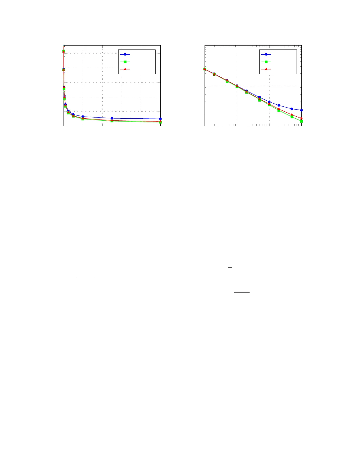
Sample-Optimal Densit y Estimation in Nearly-Linear Time Ja yadev A chary a ∗ EECS, MIT jayadev@csail.mit.edu Ilias Diakonik olas † Informatics, U. of Edinburgh ilias.d@ed.ac.uk Jerry Li ‡ EECS, MIT jerryzli@csail.mit.edu Ludwig Schmidt § EECS, MIT ludwigs@mit.edu June 3, 2015 Abstract W e design a new, fast algorithm for agnostically learning univ ariate probability distributions whose densities are w ell approximated b y piecewise p olynomial functions. Let f b e the density function of an arbitrary univ ariate distribution, and supp ose that f is OPT close in L 1 -distance to an unkno wn piecewise polynomial function with t in terv al pieces and degree d . Our algorithm dra ws n = O ( t ( d + 1) / 2 ) samples from f , runs in time e O ( n · p oly( d )) , and with probability at least 9 / 10 outputs an O ( t ) -piecewise degree- d hypothesis h that is 4 · OPT +  close to f . Our general algorithm yields (nearly) sample-optimal and ne arly-line ar time estimators for a wide range of structured distribution families o ver both con tinuous and discrete domains in a uniﬁed w a y . F or most of our applications, these are the ﬁrst sample-optimal and nearly- linear time estimators in the literature. As a consequence, our w ork resolv es the sample and computational complexities of a broad class of inference tasks via a single “meta-algorithm”. Moreo ver, w e exp erimentally demonstrate that our algorithm p erforms very w ell in practice. Our algorithm consists of three “levels”: (i) At the top level, we employ an iterative greedy algorithm for ﬁnding a goo d partition of the real line in to the pieces of a piecewise polynomial. (ii) F or each piece, w e sho w that the sub-problem of ﬁnding a go o d p olynomial ﬁt on the current in terv al can be solved eﬃciently with a separation oracle method. (iii) W e reduce the task of ﬁnding a separating h yp erplane to a com binatorial problem and giv e an eﬃcient algorithm for this problem. Com bining these three procedures giv es a densit y estimation algorithm with the claimed guarantees. ∗ Supp orted by a grant from the MIT-Shell Energy Initiativ e. † Supp orted by a Marie Curie CIG, EPSR C gran t EP/L021749/1 and a SICSA grant. ‡ Supp orted by NSF grant CCF-1217921 and DOE gran t DE-SC0008923. § Supp orted by MAD ALGO and a gran t from the MIT-Shell Energy Initiative. Con ten ts 1 In tro duction 1 1.1 Our results and techniques . . . . . . . . . . . . . . . . . . . . . . . . . . . . . . . . . 2 1.2 Related w ork . . . . . . . . . . . . . . . . . . . . . . . . . . . . . . . . . . . . . . . . 6 2 Preliminaries 7 3 P ap er outline 8 4 Iterativ e merging algorithm 10 4.1 The histogram merging algorithm . . . . . . . . . . . . . . . . . . . . . . . . . . . . . 10 4.2 The general merging algorithm . . . . . . . . . . . . . . . . . . . . . . . . . . . . . . 17 4.3 Putting ev erything together . . . . . . . . . . . . . . . . . . . . . . . . . . . . . . . . 19 5 A fast A k -pro jection oracle for p olynomials 20 5.1 The set of feasible p olynomials . . . . . . . . . . . . . . . . . . . . . . . . . . . . . . 21 5.2 Separation oracles and approximately feasible p olynomials . . . . . . . . . . . . . . . 23 5.3 Bounds on the radii of enclosing and enclosed balls . . . . . . . . . . . . . . . . . . . 24 5.4 Finding the best p olynomial . . . . . . . . . . . . . . . . . . . . . . . . . . . . . . . . 26 6 The separation oracle and the A k -computation oracle 29 6.1 Ov erview of Appr oxSepOra cle . . . . . . . . . . . . . . . . . . . . . . . . . . . . . 29 6.2 T esting non-negativit y and b oundedness . . . . . . . . . . . . . . . . . . . . . . . . . 30 6.3 An A k -computation oracle . . . . . . . . . . . . . . . . . . . . . . . . . . . . . . . . . 31 7 Applications 40 7.1 Mixture of log-conca v e distributions . . . . . . . . . . . . . . . . . . . . . . . . . . . 40 7.2 Mixture of Gaussians . . . . . . . . . . . . . . . . . . . . . . . . . . . . . . . . . . . . 41 7.3 Densities in Beso v spaces . . . . . . . . . . . . . . . . . . . . . . . . . . . . . . . . . 41 7.4 Mixtures of t -monotone distributions . . . . . . . . . . . . . . . . . . . . . . . . . . . 42 7.5 Mixtures of discrete distributions . . . . . . . . . . . . . . . . . . . . . . . . . . . . . 43 8 Exp erimen tal Ev aluation 43 8.1 Histogram h yp otheses . . . . . . . . . . . . . . . . . . . . . . . . . . . . . . . . . . . 44 8.2 Piecewise linear h yp otheses . . . . . . . . . . . . . . . . . . . . . . . . . . . . . . . . 45 A Analysis of the General Merging Algorithm: Pro of of Theorem 17 53 B A dditional Omitted Pro ofs 57 B.1 Pro of of F act 26 . . . . . . . . . . . . . . . . . . . . . . . . . . . . . . . . . . . . . . . 57 B.2 Pro of of Lemma 34 . . . . . . . . . . . . . . . . . . . . . . . . . . . . . . . . . . . . . 59 C Learning discrete piecewise p olynomials 61 C.1 Problem statement in the discrete setting . . . . . . . . . . . . . . . . . . . . . . . . 62 C.2 The algorithm in the discrete setting . . . . . . . . . . . . . . . . . . . . . . . . . . . 62 1 In tro duction Estimating an unkno wn probabilit y density function based on observed data is a classical problem in statistics that has b een studied since the late nineteenth century , starting with the pioneering w ork of Karl Pearson [Pea95]. Distribution estimation has become a paradigmatic and fundamen tal unsup ervised learning problem with a ric h history and extensiv e literature (see e.g., [BBBB72, DG85, Sil86, Sco92, DL01]). A n umber of general metho ds for estimating distributions hav e b een prop osed in the mathematical statistics literature, including histograms, kernels, nearest neighbor estimators, orthogonal series estimators, maximum likelihoo d, and more. W e refer the reader to [Ize91] for a surv ey of these techniques. During the past few decades, there has been a large b o dy of w ork on this topic in computer science with a fo cus on c omputational eﬃciency [KMR + 94, FM99, F OS05, BS10, KMV10, MV10, KSV08, VW02, DDS12a, DDS12b, DDO + 13, CDSS14a]. Supp ose that we are given a num ber of samples from an unkno wn distribution that b elongs to (or is well-appro ximated by) a giv en family of distributions C , e.g., it is a mixture of a small n umber of Gaussians. Our goal is to estimate the unknown distribution in a precise, well-deﬁned w a y . In this w ork, w e fo cus on the problem of density estimation (non-prop er learning), where the goal is to output an approximation of the unkno wn density without an y constraints on its represen tation. That is, the output h yp othesis is not necessarily a member of the family C . The “gold standard” in this setting is to design learning algorithms that are b oth statistic al ly and c omputational ly eﬃcien t. More sp eciﬁcally , the ultimate goal is to obtain estimators whose sample size is information–theoretically optimal, and whose running time is (ne arly) line ar in their sample size. An imp ortan t additional requiremen t is that our learning algorithms are agnostic or robust under mo del missp eciﬁcation, i.e., they succeed ev en if the target distribution does not belong to the giv en family C but is merely w ell-approximated by a distribution in C . W e study the problem of density estimation for univ ariate distributions, i.e., distributions with a densit y f : Ω → R + , where the sample space Ω is a subset of the real line. While densit y estimation for families of univ ariate distributions has b een studied for sev eral decades, both the sample and time complexit y w ere not y et well understo o d b efore this work, ev en for surprisingly simple classes of distributions, such as mixtures of Binomials and mixtures of Gaussians. Our main result is a general learning algorithm that can b e used to estimate a wide v ariet y of structured distribution families. F or eac h suc h family , our general algorithm simultaneously satisﬁes all three of the aforemen tioned criteria, i.e., it is agnostic, (nearly) sample optimal, and runs in ne arly-line ar time. Our algorithm is based on learning a piecewise polynomial function that appro ximates the unkno wn density . The approac h of using piecewise p olynomial approximation has b een employ ed in this context b efore — our main contribution is to impro ve the computational complexity of this metho d and to mak e it nearly-optimal for a wide range of distribution families. The k ey idea of using piecewise p olynomials for learning is that the existenc e of go o d piecewise p olynomial approximations for a family C of distributions can be leveraged for the design of eﬃcien t learning algorithms for the family C . The main algorithmic ingredient that makes this metho d p ossible is an eﬃcient pro cedure for agnostically learning piecewise p olynomial density functions. In prior work, Chan, Diak onikolas, Serv edio, and Sun [CDSS14a] obtained a nearly-sample optimal and p olynomial time algorithm for this learning problem. Unfortunately , how ev er, the p olynomial exp onent in their running time is quite high, whic h mak es their algorithm prohibitively slow for most applications. In this pap er, we design a new, fast algorithm for agnostically learning piecewise p olynomial distributions, which in turn yields sample-optimal and ne arly-line ar time estimators for a wide range of structured distribution families ov er b oth contin uous and discrete domains. F or most of our 1 applications, these are the ﬁrst sample-optimal and nearly-linear time estimators in the literature. As a consequence, our w ork resolves the sample and computational complexit y of a broad class of inference tasks via a single “meta-algorithm”. Moreo ver, we exp erimen tally demonstrate that our algorithm p erforms very w ell in practice. W e stress that a signiﬁcant n umber of new algorithmic and tec hnical ideas are needed for our main result, as we explain next. 1.1 Our results and techniques In this section, w e describe our results in detail, compare them to prior work, and give an ov erview of our new algorithmic ideas. Preliminaries. W e consider univ ariate probabilit y densit y functions (p df ’s) deﬁned ov er a kno wn ﬁnite interv al I ⊆ R . (W e remark that this assumption is without loss of generalit y and our results easily apply to densities deﬁned o ver the entire real line.) W e fo cus on a standard notion of learning an unknown probabilit y distribution from sam- ples [KMR + 94], which is a natural analogue of V aliant’s well-kno wn P AC mo del for learning Bo olean functions [V al84] to the unsup ervised setting of learning an unkno wn probabilit y distribution. (W e remark that our deﬁnition is essentially equiv alent to the notion of the L 1 minimax rate of conv er- gence in statistics [DL01].) A distribution learning problem is deﬁned by a class C of probability distributions ov er a domain Ω . Given  > 0 and sample access to an unknown distribution with den- sit y f , the goal of an agnostic le arning algorithm for C is to compute a hypothesis h suc h that, with probabilit y at least 9 / 10 , it holds k h − f k 1 ≤ C · OPT C ( f ) + , where OPT C ( f ) := inf q ∈C k q − f k 1 , i.e., OPT C ( f ) is the L 1 -distance b etw een the unkno wn density f and the closest distribution to it in C , and C ≥ 1 is a univ ersal constan t. W e sa y that a function f o ver an interv al I is a t -pie c ewise de gr e e- d p olynomial if there is a partition of I in to t disjoin t interv als I 1 , . . . , I t suc h that f ( x ) = f j ( x ) for all x ∈ I j , where eac h of f 1 , . . . , f t is a p olynomial of degree at most d . Let P t,d ( I ) denote the class of all t -piecewise degree- d p olynomials o v er the in terv al I . Our Results. Our main algorithmic result is the follo wing: Theorem 1 (Main) . L et f : I → R + b e the density of an unknown distribution over I , wher e I is either an interval or the discr ete set [ N ] . Ther e is an algorithm with the fol lowing p erformanc e guar ante e: Given p ar ameters t, d ∈ Z + , an err or toler anc e  > 0 , and any γ > 0 , the algorithm dr aws n = O γ ( t ( d + 1) / 2 ) samples fr om the unknown distribution, runs in time e O ( n · p oly( d + 1)) , and with pr ob ability at le ast 9 / 10 outputs an O ( t ) -pie c ewise de gr e e- d hyp othesis h such that k f − h k 1 ≤ (3 + γ )OPT t,d ( f ) +  , wher e OPT t,d ( f ) := inf r ∈P t,d ( I ) k f − r k 1 is the err or of the b est t -pie c ewise de gr e e- d appr oximation to f . In prior work, [CDSS14a] ga ve a learning algorithm for this problem that uses e O ( t ( d + 1) / 2 ) samples and runs in p oly( t, d + 1 , 1 / ) time. W e stress that the algorithm of [CDSS14a] is pro- hibitiv ely slow. In particular, the running time of their approach is e Ω( t 3 · ( d 3 . 5 / 3 . 5 + d 6 . 5 / 2 . 5 )) , whic h renders their result more of a “pro of of principle” than a computationally eﬃcien t algorithm. This prompts the follo wing question: Is such a high running time ne c essary to achieve this level of sample eﬃciency? Ideally , one w ould lik e a sample-optimal algorithm with a low-order p olynomial running time (ideally , linear). Our main result sho ws that this is indeed p ossible in a very strong sense. The running time of our algorithm is line ar in t/ 2 (up to a log (1 / ) factor), which is essentially the b est p ossible; the p olyno- mial dep endence on d is e O ( d 3+ ω ) , where ω is the matrix multiplication exp onent. This substantially 2 impro ved running time is of critical imp ortance for the applications of Theorem 1. Moreo ver, the sample complexity of our algorithm remo v es the extraneous logarithmic factors presen t in the sam- ple complexity of [CDSS14a] and matches the information-theoretic lo wer b ound up to a constan t factor. As we explain b elow, Theorem 1 leads to (nearly) sample-optimal and ne arly-line ar time estimators for a wide range of natural and w ell-studied families. F or most of these applications, ours is the ﬁrst estimator with sim ultaneously nearly optimal sample and time complexit y . Our new algorithm is clean and modular. As a result, Theorem 1 also applies to discrete distributions ov er an ordered domain (e.g., [ N ] ). The approach of [CDSS14a] do es not extend to p olynomial approximation o ver discrete domains, and designing such an algorithm was left as an op en problem in their w ork. As a consequence, w e obtain sev eral new applications to learning mixtures of discrete distributions. In particular, w e obtain the ﬁrst nearly sample optimal and nearly-linear time estimators for mixtures of Binomial and P oisson distributions. T o the b est of our knowledge, no p olynomial time algorithm with nearly optimal sample complexit y w as kno wn for these basic learning problems prior to this work. Applications. W e no w explain ho w to use Theorem 1 in order to agnostically learn structured distribution families. Given a class C that w e w ant to learn, w e proceed as follows: (i) Pro ve that an y distribution in C is / 2 -close in L 1 -distance to a t -piecewise degree- d p olynomial, for appropriate v alues of t and d . (ii) Use Theorem 1 for these v alues of t and d to agnostically learn the target distribution up to error / 2 . Note that t and d will dep end on the desired error  and the underlying class C . W e emphasize that there are man y com binations of t and d that guarantee an / 2 -appro ximation of C in Step (i). T o minimize the sample complexity of our learning algorithm in Step (ii), we would like to determine the v alues of t and d that minimize the pro duct t ( d + 1) . This is, of course, an approximation theory problem that depends on the structure of the family C . F or example, if C is the family of log-concav e distributions, the optimal t -histogram appro xima- tion with accuracy  requires Θ(1 / ) interv als. This leads to an algorithm with sample complexity Θ(1 / 3 ) . On the other hand, it can b e sho wn that any log-concav e distribution has a piecewise line ar  -appro ximation with Θ(1 / 1 / 2 ) interv als [CDSS14a, DK15], whic h yields an algorithm with sample complexit y Θ(1 / 5 / 2 ) . P erhaps surprisingly , this sample b ound cannot b e improv ed using higher degree piecewise p olynomials; one can sho w an information-theoretic lo wer bound of Ω(1 / 5 / 2 ) for learning log-concav e densities [DL01]. Hence, Theorem 1 giv es a sample-optimal and nearly-linear time agnostic learning algorithm for this fundamental problem. W e remark that piecewise p olyno- mial approximations are “closed” under taking mixtures. As a corollary , Theorem 1 also yields an O ( k / 5 / 2 ) sample and nearly-linear time algorithm for learning an arbitrary mixture of k log-concav e distributions. Again, there exists a matching information-theoretic low er bound of Ω( k / 5 / 2 ) . As a second example, let C b e the class of mixtures of k Gaussians in one dimension. It is not diﬃcult to show that learning such a mixture of Gaussians up to L 1 -distance  requires Ω( k / 2 ) samples. By approximating the corresp onding probability density functions with piecewise p olynomials of degree O (log(1 / )) , w e obtain an agnostic learning algorithm for this class that uses n = e O ( k / 2 ) samples and runs in time e O ( n ) . Similar b ounds can b e obtained for several other natural parametric mixture families. Note that for a wide range of structured families, 1 the optimal c hoice of the degree d (i.e., the c hoice minimizing t ( d + 1) among all / 2 -approximations) will b e at most p oly-lo garithmic in 1 / . F or 1 This includes all structured families considered in [CDSS14a] and several previously-studied distributions not co vered by [CDSS14a]. 3 sev eral classes (such as unimo dal, monotone hazard rate, and log-conca ve distributions), the degree d is ev en a constant. As a consequence, Theorem 1 yields (nearly) sample optimal and nearly-linear time estimators for all these families in a uniﬁed w ay . In particular, w e obtain sample optimal (or nearly sample optimal) and nearly-linear time estimators for a wide range of structured distribution families, including arbitrary mixtures of natural distributions suc h as multi-modal, concav e, conv ex, log-conca ve, monotone hazard rate, Gaussian, P oisson, Binomial, functions in Beso v spaces, and others. See T able 1 for a summary of these applications. F or eac h distribution family in the table, we pro vide a comparison to the b est previous result. Note that w e do not aim to exhaustively co ver all p ossible applications of Theorem 1, but rather to give some selected applications that are indicativ e of the generalit y and p ow er of our metho d. Moreo ver, our non-prop er learning algorithm is also useful for prop er learning. Indeed, Theo- rem 1 has recen tly b een used [LS15] as a crucial comp onen t to obtain the fastest kno wn agnostic algorithm for prop erly learning a mixture of univ ariate Gaussian distributions. Note that non-proper learning and prop er learning for a family C are equiv alent in terms of sample complexity: given any (non-prop er) h yp othesis, we can p erform a brute-force search to ﬁnd its closest appro ximation in the class C . The c hallenging part is to p erform this computation eﬃcien tly . Roughly sp eaking, given a piecewise polynomial h yp othesis, [LS15] design an eﬃcien t algorithm to ﬁnd the closest mixture of k Gaussians. Our T echniques. W e now pro vide a brief o verview of our new algorithm and tec hniques in parallel with a comparison to the previous algorithm of [CDSS14a]. W e require the follo wing deﬁnition. F or any k ≥ 1 and an in terv al I ⊆ R , deﬁne the A k -norm of a function g : I → R to be k g k A k def = sup I 1 ,...,I k k X i =1 | g ( I i ) | , where the supremum is ov er all sets of k disjoint interv als I 1 , . . . , I k in I , and g ( J ) def = R J g ( x ) d x for an y measurable set J ⊆ I . Our main probabilistic tool is the following w ell-kno wn version of the V C inequality: Theorem 2 (V C Inequalit y [VC71, DL01]) . L et f : I → R + b e an arbitr ary p df over I , and let b f b e the empiric al p df obtaine d after taking n i.i.d. samples fr om f . Then E [ k f − b f k A k ] ≤ O r k n ! . Giv en this theorem, it is not diﬃcult to sho w that the follo wing tw o-step pro cedure is an agnostic learning algorithm for P t,d : (1) Dra w a set of n = Θ( t ( d + 1) / 2 ) samples from f ; (2) Output the piecewise-p olynomial h yp othesis h ∈ P t,d that minimizes the quan tit y k h − b f k A k up to an additive error of O (  ) , where k = O ( t ( d + 1)) . W e remark that the optimization problem in Step (2) is non-conv ex. Ho wev er, it has suﬃcient structure so that it can b e solv ed in p olynomial time. Intuitiv ely , an algorithm for Step (2) in volv es t wo main ingredients: 4 Class of distributions Sample complexit y Time complexit y Reference Optimalit y t -histograms e O ( t  2 ) e O ( t  2 ) [CDSS14b] O ( t  2 ) O ( t  2 log(1 / )) Theorem 10 S O , T O S t -piecewise degree- d polynomials e O ( t · d  2 ) e O  t 3 · ( d 3 . 5  3 . 5 + d 6 . 5  2 . 5 )  [CDSS14a] O ( t · d  2 ) e O ( t · d ω +3  2 ) Theorem 1 N S O k -mixture of log-conca v e e O ( k  5 / 2 ) e O ( k 3  5 ) [CDSS14a] O ( k  5 / 2 ) e O ( k  5 / 2 ) Theorem 42 S O , N T O k -mixture of Gaussians e O ( k  2 ) e O ( k 3  3 . 5 ) [CDSS14a] O ( k log (1 / )  2 ) e O ( k  2 ) Theorem 43 N S O , N T O Beso v space B α q ( L p ([0 , 1])) O α  log 2 (1 / )  2+1 /α  e O α  1  6+3 /α  [WN07] O α  1  2+1 /α  e O α  1  2+1 /α  Theorem 44 S O , N T O k -mixture of t -monotone e O ( t · k  2+1 /t ) e O ( k 3  3 /t · ( t 3 . 5  3 . 5 + t 6 . 5  2 . 5 )) [CDSS14a] O ( t · k  2+1 /t ) e O ( k · t 2+ ω  2+1 /t ) Theorem 45 S O , N T O for t = 1 , 2 k -mixture of t -modal e O ( t · k log ( N )  3 ) e O ( t · k log ( N )  3 ) [CDSS14b] O ( t · k log ( N )  3 ) O ( t · k log ( N )  3 log(1 / )) Theorem 46 S O , T O S k -mixture of MHR e O ( k log ( N/ )  3 )) e O ( k log ( N/ )  3 )) [CDSS14b] O ( k log ( N/ )  3 ) O ( k log ( N/ )  3 log(1 / )) Theorem 47 S O , T O S k -mixture of Binomial, P oisson e O ( k  3 ) e O ( k  3 ) [CDSS14b] O ( k log (1 / )  2 ) e O ( k  2 ) Theorem 48 N S O , N T O S O : Sample complexit y is optimal up to a constant factor. N S O : Sample complexit y is optimal up to a p oly-logarithmic factor. T O S : Time complexit y is optimal (up to sorting the samples). N T O : Time complexity is optimal up to a p oly-logarithmic factor. T able 1: A list of applications to agnostically learning sp eciﬁc families of distributions. F or each class, the ﬁrst row is the b est known previous result and the second row is our result. Note that for most of the examples, our algorithm runs in time that is nearly-linear in the information-theoretically optimal sample complexit y . The last three classes are o ver discrete sets, and N denotes the size of the support. (2.1) An eﬃcien t pro cedure to ﬁnd a go o d set t interv als. (2.2) An eﬃcient pro cedure to agnostically learn a degree- d p olynomial in a giv en sub-interv al of the domain. W e remark that the pro cedure for (2.1) will use the pro cedure for (2.2) multiple times as a subroutine. [CDSS14a] solv e an appropriately relaxed version of Step (2) b y a combination of linear pro- 5 gramming and dynamic programming. Roughly sp eaking, they formulate a p olynomial size linear program to agnostically learn a degree- d p olynomial in a given in terv al, and use a dynamic pro- gram in order to disco ver the correct t in terv als. It should b e emphasized that the algorithm of [CDSS14a] is theoretically eﬃcien t (p olynomial time), but prohibitively slow for real applica- tions with large data sets. In particular, the linear program of [CDSS14a] has Ω( d/ ) v ariables and Ω( d 2 / 2 + d 5 / ) constraints. Hence, the running time of their algorithm using the fastest kno wn LP solv er for their instance [LS14] is at least e Ω( d 3 . 5 / 3 . 5 + d 6 . 5 / 2 . 5 ) . Moreov er, the dynamic pro- gram to implement (2) has running time at least Ω( t 3 ) . This leads to an ov erall running time of e Ω  t 3 · ( d 3 . 5 / 3 . 5 + d 6 . 5 / 2 . 5 )  , which quic kly b ecomes unrealistic even for mo dest v alues of , t , and d . W e no w provide a sk etch of our new algorithm. A t a high-level, w e implemen t pro cedure (2.1) ab o ve using an iter ative gr e e dy algorithm. Our algorithm circum v ents the need for a dynamic programming approach as follo ws: The main idea is to iteratively merge pairs of in terv als by calling an oracle for pro cedure (2.2) in every step until the num b er of interv als b ecomes O ( t ) . Our iterative algorithm and its subtle analysis are directly inspired by the V C inequality . Roughly sp eaking, in eac h iteration the algorithm estimates the con tribution to an appropriate notion of error when t wo consecutiv e interv als are merged, and it merges pairs of interv als with small error. This pro cedure ensures that the n umber of in terv als in our partition decreases geometrically with the num b er of iterations. Our algorithm for pro cedure (2.2) is based on conv ex programming and runs in time p oly ( d + 1) / 2 (note that the dependence on  is optimal). T o achiev e this signiﬁcan t running time improv e- men t, we use a nov el approac h that is quite diﬀerent from that of [CDSS14a]. Roughly sp eaking, w e are able to exploit the problem structure inherent in the A k optimization problem in order to separate the problem dimension d from the problem dimension 1 / , and only solve a con vex program of dimension d (as opp osed to dimension p oly( d/ ) in [CDSS14a]). More speciﬁcally , w e consider the conv ex set of non-negative p olynomials with A d +1 distance at most τ from the empirical distri- bution. While this set is deﬁned through a large n umber of constrain ts, w e sho w that it is p ossible to design a separation oracle that runs in time ne arly line ar in b oth the num b er of samples and the degree d . Com bined with to ols from conv ex optimization suc h as the Ellipsoid metho d or V aidy a’s algorithm, this giv es an eﬃcient algorithm for pro cedure (2.2). 1.2 Related w ork There is a long history of researc h in statistics on estimating structured families of distributions. F or distributions o v er con tin uous domains, a very natural t yp e of structure to consider is some sort of “shap e constraint” on the probabilit y densit y function (pdf ) deﬁning the distribution. Statistical researc h in this area started in the 1950’s, and the reader is referred to the b o ok [BBBB72] for a sum- mary of the early w ork. Most of the literature in shape-constrained densit y estimation has fo cused on one-dimensional distributions, with a few exceptions during the past decade. V arious structural restrictions hav e b een studied o ver the years, starting from monotonicit y , unimo dalit y , conv exit y , and conca vit y [Gre56, Bru58, Rao69, W eg70, HP76, Gro85, Bir87a, Bir87b, F ou97, CT04, JW09], and more recen tly focusing on structural restrictions suc h as log-conca vit y and k -monotonicit y [BW07, DR09, BR W09, GW09, BW10, KM10, W al09, D W13, CS13, KS14, BD14, HW15]. The reader is referred to [GJ14] for a recen t bo ok on the sub ject. Mixtures of structured distributions ha ve received muc h atten tion in statistics [Lin95, R W84, TSM85, LB99] and, more recen tly , in theoretical computer science [Das99, DS00, AK01, VW02, FOS05, AM05, MV10]. 6 The most common metho d used in statistics to address shap e-constrained inference problems is the Maxim um Lik eliho o d Estimator (MLE) and its v arian ts. While the MLE is v ery p opular and quite natural, we note that it is not agnostic, and it may in general require solving an in tractable optimization problem (e.g., for the case of mixture mo dels.) Piecewise p olynomials (splines) ha ve b een extensively used as to ols for inference tasks, including densit y estimation, see, e.g., [WW83, WN07, Sto94, SHKT97]. W e remark that splines in the statistics literature hav e b een used in the context of the MLE, whic h is very diﬀerent than our approac h. Moreo v er, the degree of the splines used is t ypically b ounded by a small constant and the underlying algorithms are heuristic in most cases. A related line of w ork in mathematical statistics [KP92, DJKP95, KPT96, DJKP96, DJ98] uses non-linear estimators based on w av elet tec hniques to learn contin uous distributions whose densities satisfy v arious smo othness constraints, suc h as T rieb el and Besov-t yp e smoothness. W e remark that the focus of these w orks is usually on the statistical eﬃciency of the prop osed estimators. F or the problem of learning piecewise constant distributions with t unknown interv al pieces, [CDSS14b] recen tly gav e an n = e O ( t/ 2 ) sample and e O ( n ) time algorithm. Ho wev er, their approach do es not seem to generalize to higher degrees. Moreo v er, recall that Theorem 1 remo ves all loga- rithmic factors from the sample complexit y . F urthermore, our algorithm runs in time proportional to the time required to sort the samples, while their algorithm has additional logarithmic factors in the running time (see T able 1). Our iterative merging idea is quite robust: together with Hegde, the authors of the current pap er hav e shown that an analogous approach yields sample optimal and eﬃcient algorithms for agnostically learning discrete distributions with piecewise constant functions under the  2 -distance metric [ADH + 15]. W e emphasize that learning under the  2 -distance is easier than under the L 1 - distance, and that the analysis of [ADH + 15] is signiﬁcantly simpler than the analysis in the curren t pap er. Moreo v er, the algorithmic subroutine of ﬁnding a go o d p olynomial ﬁt on a ﬁxed interv al required by the  2 algorithm is substantially simpler than the subroutine we require here. Indeed, in our case, the asso ciated optimization problem has exp onentially man y linear constraints, and th us cannot be fully describ ed, ev en in polynomial time. P ap er Structure. After some preliminaries in Section 2, w e giv e an outline of our algorithm in Section 3. Sections 4 – 6 contain the v arious comp onen ts of our algorithm. Section 7 gives a detailed description of our applications to learning structured distribution families, and we conclude in Section 8 with our exp erimen tal ev aluation. 2 Preliminaries W e consider univ ariate probabilit y density functions (p df ’s) deﬁned o ver a known ﬁnite interv al I ⊆ R . F or an interv al J ⊆ I and a p ositive in teger k , w e will denote by I k J the family of all sets of k disjoin t interv als I 1 , . . . , I k where each I i ⊆ J . F or a measurable function g : I → R and a measurable set S , let g ( S ) def = R S g . The L 1 -norm of g ov er a subinterv al J ⊆ I is deﬁned as k g k 1 ,J def = R J | g ( x ) | dx . More generally , for an y set of disjoint in terv als J ∈ I k I , w e deﬁne k g k 1 , J = P J ∈J k g k 1 ,J . W e no w deﬁne a norm whic h induces a corresp onding distance metric that will b e crucial for this paper: Deﬁnition 3 ( A k -norm) . L et k b e a p ositive inte ger and let g : I → R b e me asur able. F or any 7 subinterval J ⊆ I , the A k -norm of g on J is deﬁne d as k g k A k ,J def = sup I ∈ I k J X M ∈I | g ( M ) | . When J = I , we omit the se c ond subscript and simply write k g k A k . Mor e gener al ly, for any set of disjoint intervals J = { J 1 , . . . , J ` } wher e e ach J i ⊆ I , we deﬁne k g k A k , J = sup I X J ∈I | g ( J ) | wher e the supr emum is taken over al l I ∈ I k J such that for al l J ∈ I ther e is a J i ∈ J with J ⊆ J i . W e note that the deﬁnition of the A k -norm in this work is slightly diﬀerent than that in [DL01, CDSS14a] but is easily seen to b e essentially equiv alen t. The VC inequality (Theorem 2) along with uniform conv ergence b ounds (see, e.g., Theorem 2.2. in [CDSS13] or p. 17 in [DL01]), yields the follo wing: Corollary 4. Fix 0 <  and δ < 1 . L et f : I → R + b e an arbitr ary p df over I , and let b f b e the empiric al p df obtaine d after taking n = Θ(( k + log 1 /δ ) / 2 ) i.i.d. samples fr om f . Then with pr ob ability at le ast 1 − δ , k f − b f k A k ≤  . Deﬁnition 5. L et g : I → R . W e say that g has at most k sign changes if ther e exists a p artition of I into intervals I 1 , . . . , I k +1 such that for al l i ∈ [ k + 1] either g ( x ) ≥ 0 for al l x ∈ I i or g ( x ) ≤ 0 for al l x ∈ I i . W e will need the follo wing elemen tary facts about the A k -norm. Fact 6. L et J ⊆ I b e an arbitr ary interval or a ﬁnite set of intervals. L et g : I → R b e a me asur able function. (a) If g has at most k − 1 sign changes in J , then k g k 1 ,J = k g k A k ,J . (b) F or al l k ≥ 1 , we have k g k A k ,J ≤ k g k 1 ,J . (c) L et α b e a p ositive inte ger. Then, k g k A α · k ,I ≤ α · k g k A k ,I . (d) L et f : I → R + b e a p df over I , and let J 1 , . . . , J ` b e ﬁnite sets of disjoint subintervals of I , such that for al l i, i 0 and for al l I ∈ J i and I 0 ∈ J i 0 , I and I 0 ar e disjoint. Then, for al l p ositive inte gers m 1 , . . . , m ` , P ` i =1 k f k A m i , J i ≤ k f k A M , wher e M = P ` i =1 m i . 3 P ap er outline In this section, w e giv e a high-level description of our algorithm for learning t -piecewise degree- d p oly onomials. Our algorithm can b e divided into three lay ers. 8 Lev el 1: General merging (Section 4). A t the top lev el, we design an iterativ e merging algorithm for ﬁnding the closest piecewise p olynomial approximation to the unknown target densit y . Our merging algorithm applies more generally to broad classes of piecewise h yp otheses. Let D b e a class of h yp otheses satisfying the follo wing: (i) The num b er of intersections b etw een any tw o h yp otheses in D is b ounded. (ii) Given an interv al J and an empirical distribution b f , we can eﬃcien tly ﬁnd the b est ﬁt to b f from functions in D with resp ect to the A k -distance. (iii) W e can eﬃcien tly compute the A k -distance b etw een the empirical distribution and an y h yp othesis in D . Under these assumptions, our merging algorithm agnostically learns piecewise hypotheses where eac h piece is in the class D . In Section 4.1, we start b y presenting our merging algorithm for the case of piecewise constant h yp otheses. This in teresting sp ecial case captures many of the ideas of the general case. In Section 4.2, we pro ceed to present our general merging algorithm that applies all classes of distributions satisfying properties (i)-(iii). When w e adapt the general merging algorithm to a new class of piecewise hypotheses, the main algorithmic c hallenge is constructing a pro cedure for prop erty (ii). More formally , we require a pro cedure with the following guarantee. Deﬁnition 7. Fix η > 0 . An algorithm O p ( b f , J, η ) is an η -approximate A k -pro jection oracle for D if it takes as input an interval J and b f , and r eturns a hyp othesis h ∈ D such that k h − b f k A k ≤ inf h 0 ∈D k h 0 − b f k A k ,J + η . One of our main con tributions is an eﬃcient A k -pro jection oracle for the class of degree- d p olynomials, whic h w e describ e next. Lev el 2: A k -pro jection for p olynomials (Section 5). Our A k -pro jection oracle computes the co eﬃcien ts c ∈ R d +1 of a degree- d p olynomial p c that approximately minimizes the A k -distance to the empirical distribution b f in the giv en interv al J . Moreov er, our oracle ensures that p c is non-negativ e on J . A t a high-lev el, we formulate the A k -pro jection as a conv ex optimization problem. A k ey insight is that w e can construct an eﬃcient, appro ximate sep ar ation or acle for the set of p olynomials that ha ve an A k -distance of at most τ to the empirical distribution b f . Combining this separation oracle with existing conv ex optimization algorithms allows us to solve the feasibilit y problem of c hecking whether we can achiev e a given A k -distance τ . W e then conv ert the feasibilit y problem to the optimization v ariant via a binary searc h o ver τ . Note that the set of non-negative p olynomials is a sp ectrahedron (the feasible set of a semideﬁnite program). After restricting the set of co eﬃcien ts to non-negativ e p olynomials, we can simplify the deﬁnition of the A k -distance: it suﬃces to consider sets of interv als with endpoints at the lo cations of samples. Hence, we can replace the supremum in the deﬁnition of the A k -distance by a maxim um o ver a ﬁnite set, which sho ws that the set of p olynomials that are b oth non-negative and τ -close to b f in A k -distance is also a sp ectrahedron. This suggests that the A k -pro jection problem could b e solved b y a black-box application of an SDP solver. How ev er, this would lead to a running time that is exp onential in k b ecause there are more than  s 2 k  p ossible sets of in terv als, where s is the n umber of sample points in the current interv al J . 2 2 While the authors of [CDSS14a] introduce an enco ding of the A k -constrain t with fewer linear inequalities, their 9 Instead of using black-box SDP or LP solvers, w e construct an algorithm that exploits additional structure in the A k -pro jection problem. Most importantly , our algorithm separates the dimension of the desired degree- d p olynomial from the num b er of samples (or equiv alently , the error parameter  ). This allo ws us to achiev e a running time that is ne arly-line ar for a wide range of distributions. In terestingly , w e can solve our SDP signiﬁcan tly faster than the LP whic h has b een prop osed in [CDSS14a] for the same problem. W e ac hieve this by combining V aidya’s cutting plane metho d [V ai96] with an eﬃcien t separation oracle that leverages the structure of the A k -distance. This separation oracle is the third lev el of our algorithm, which w e describe next. Lev el 3: A k -separation oracle for p olynomials (Section 6). Our separation oracle eﬃciently tests t wo prop erties for a given p olynomial p c with co eﬃcien ts c ∈ R d +1 : (i) Is the p olynomial p c non-negativ e on the given interv al J ? (ii) Is the A k -distance b etw een p c and the empirical distribution b f at most τ ? W e implement T est (i) by using known algorithms for ﬁnding ro ots of real p olynomials eﬃcien tly [P an01]. Note, ho wev er, that ro ot-ﬁnding algorithms cannot b e exact for degrees larger than 4 . Hence, w e can only approximately T est (i), whic h necessarily leads to an appr oximate separation oracle. Nev ertheless, we sho w that such an appro ximate oracle is still suﬃcien t for solving the conv ex program outlined ab ov e. A t a high lev el, our algorithm pro ceeds as follo ws. W e ﬁrst verify that our current candidate p olynomial p c is “nearly” non-negative at ev ery p oin t in J . Assuming that p c passes this test, w e then fo cus on the problem of computing the A k -distance b etw een p c and b f . W e reduce this problem to a discrete v arian t by showing that the endp oints of interv als jointly maximizing the A k -distance are guaran teed to coincide with sample points of the empirical distribution (assuming p c is nearly non-negative on the current in terv al). Our discrete v arian t of this problem is related to a previously studied question in computational biology , namely ﬁnding maxim um-scoring DNA segmen t sets [Csu04]. W e exploit this connection and giv e a com binatorial algorithm for this discrete v ariant that runs in time nearly-linear in the n um b er of sample p oints in J and the degree d . Once w e hav e found a set of interv als maximizing the A k -distance, w e can con vert it to a separating h yp erplane for the polynomial co eﬃcien ts c and the set of non-negativ e p olynomials with A k - distance at most τ to b f . Com bining these ingredien ts yields our general algorithm with the p erformance guaran tees stated in Theorem 1. 4 Iterativ e merging algorithm In this section, w e describ e and analyze our iterativ e merging algorithm. W e start with the case of histograms and then provide the generalization to piecewise polynomials. 4.1 The histogram merging algorithm A t -histo gr am is a function h : I → R that is piecewise constan t with at most t in terv al pieces, i.e., there is a partition of I into interv als I 1 , . . . , I t 0 with t 0 ≤ t suc h that h is constant on each I i . Giv en sample access to an arbitrary p df f o ver I and a p ositiv e integer t , we would like to approac h increases the num b er of v ariables in the optimization problem to dep end p olynomially on 1 / , which leads to an Ω(p oly ( d + 1) / 3 . 5 ) running time. In contrast, our approach achiev es a nearly optimal dep endence on  that is e O (poly ( d + 1) / 2 ) . 10 eﬃcien tly compute a go o d t -histogram approximation to f . Namely , if H t = H t ( I ) denotes the set of t -histogram probabilit y density functions ov er I and OPT t = inf g ∈H t k g − f k 1 , our goal is to output an O ( t ) -histogram h : I → R that satisﬁes k h − f k 1 ≤ C · OPT t + O (  ) with high probability o ver the samples, where C is a univ ersal constant. The follo wing notion of ﬂattening a function o ver an interv al will b e crucial for our algorithm: Deﬁnition 8. F or a function g : I → R and an interval J = [ u, v ] ⊆ I , we deﬁne the ﬂattening of g o v er J , denote d g J , to b e the c onstant function deﬁne d on J as g J ( x ) def = g ( J ) v − u for al l x ∈ J. F or a set I of disjoint intervals in I , we deﬁne the ﬂattening of g ov er I to b e the function g I on ∪ J ∈I J which for e ach J ∈ I satisﬁes g I ( x ) = g J ( x ) for al l x ∈ J . W e start b y providing an in tuitive explanation of our algorithm follow ed by a pro of of correctness. The algorithm draws n = Θ(( t + log 1 /δ ) / 2 ) samples x 1 ≤ x 2 ≤ . . . ≤ x n from f . W e start with the follo wing partition of I = [ a, b ] : I 0 = { [ a, x 1 ) , [ x 1 , x 1 ] , ( x 1 , x 2 ) , [ x 2 , x 2 ] , . . . , ( x n − 1 , x n ) , [ x n , x n ] , ( x n , b ] } . (1) This is the partition where eac h in terv al is either a single sample point or the interv al betw een t w o consecutiv e samples. Starting from this partition, our algorithm greedily merges pairs of consecutive in terv als in a sequence of iterations. When deciding whic h interv al pairs to merge, the following notion of appro ximation error will b e crucial: Deﬁnition 9. F or a function g : I → R and an interval J ⊆ I , deﬁne e ( g , J ) = k g − g J k A 1 ,J . W e c al l this quantity the A 1 -error of g on J . In the j -th iteration, given the curren t in terv al partition I j , we greedily merge pairs of consecu- tiv e interv als to form the new partition I j +1 . Let s j b e the num b er of in terv als in I j . In particular, giv en I j = { I 1 ,j , . . . , I s j ,j } , w e consider the interv als I 0 `,j +1 = I 2 ` − 1 ,j ∪ I 2 `,j for all 1 ≤  ≤ s j / 2 . 3 W e ﬁrst iterate through 1 ≤  ≤ s j / 2 and calculate the quantities e `,j = e ( b f , I 0 `,j +1 ) , i.e., the A 1 -errors of the empirical distribution on the candidate interv als. T o construct I j +1 , the algorithm k eeps track of the largest O ( t ) errors e `,j . F or eac h  with e `,j b eing one of the O ( t ) largest errors, w e do not merge the corresponding in terv als I 2 ` − 1 ,j and I 2 `,j . That is, w e include I 2 ` − 1 ,j and I 2 `,j in the new partition I j +1 . Otherwise, we include their union I 0 `,j +1 in I j +1 . W e p erform this pro cedure O (log 1  ) times and arriv e at some ﬁnal partition I . Our output h yp othesis is the ﬂattening of b f with resp ect to I . F or a formal description of our algorithm, see the pseudo co de given in Algorithm 1 b elo w. In addition to the parameter t , the algorithm has a parameter α ≥ 1 that con trols the trade-oﬀ b et ween the approximation ratio C ac hieved b y the algorithm and the num ber of pieces in the output histogram. The following theorem characterizes the p erformance of Algorithm 1, establishing the sp ecial case of Theorem 1 corresp onding to d = 0 . 3 W e assume s j is even for simplicity . 11 Algorithm 1 Appro ximating with histograms b y merging. 1: function Constr uctHistogram ( f , t, α, , δ ) 2: Dra w n = Θ(( αt + log 1 /δ ) / 2 ) samples x 1 ≤ x 2 ≤ . . . ≤ x n . 3: F orm the empirical distribution b f from these samples. 4: Let I 0 ← { [ a, x 1 ) , [ x 1 , x 1 ] , ( x 1 , x 2 ) , . . . , ( x n − 1 , x n ) , [ x n , x n ] , ( x n , b ] } be the initial partition. 5: j ← 0 6: while |I j | > 2 α · t do 7: Let I j = { I 1 ,j , I 2 ,j , . . . , I s j − 1 ,j , I s j ,j } 8: for  ∈ { 1 , 2 , . . . , s j 2 } do 9: I 0 `,j +1 ← I 2 ` − 1 ,j ∪ I 2 `,j 10: e `,j ← e ( b f , I 0 `,j +1 ) 11: end for 12: Let L be the set of  ∈ { 1 , 2 , . . . , s j 2 } with the αt largest errors e `,j . 13: Let M b e the complement of L . 14: I j +1 ← S ` ∈ L { I 2 ` − 1 ,j , I 2 `,j } 15: I j +1 ← I j +1 ∪ { I 0 `,j +1 |  ∈ M } 16: j ← j + 1 17: end while 18: return I = I j and the ﬂattening b f I 19: end function Theorem 10. Algorithm ConstructHistogram ( f , t, α, , δ ) dr aws n = O (( αt + log 1 /δ ) / 2 ) sam- ples fr om f , runs in time O ( n (log (1 / ) + log log(1 /δ ))) , and outputs a hyp othesis h and a c orr e- sp onding p artition I of size |I | ≤ 2 α · t such that with pr ob ability at le ast 1 − δ we have k h − f k 1 ≤ 2 · OPT t + 4 · OPT t + 4  α − 1 +  . (2) Pr o of. W e start b y analyzing the running time. T o this end, w e sho w that the n umber of in terv als decreases exp onentially with the num b er of iterations. In the j -th iteration, we merge all but αt in terv als. Therefore, s j +1 = αt + s j − α t 2 = 3 s j 4 + 2 αt − s j 4 . Note that the algorithm enters the while lo op when s j > 2 αt , implying that s j +1 < 3 s j 4 . By construction, the num ber of interv als is at least αt when the algorithm exits the while lo op. Therefore, the n um b er of iterations of the while lo op is at most O  log n αt  = O (log(1 / ) + log log (1 /δ )) , whic h follo ws by substituting the v alue of n from the statemen t of the theorem. W e no w show that eac h iteration tak es time O ( n ) . Without loss of generality , assume that we compute the A 1 -distance only o ver interv als ending at a data sample. F or an interv al J = [ c, d ] containing m sample p oin ts, 12 x 1 , . . . , x m , let C j = ( x j − x 1 ) j n − ( d − c ) n . The A 1 -error of b f on J is given b y max C j − min C j and can therefore b e computed in time prop ortional to the num b er of sample p oints in the interv al. Therefore, the total time of the algorithm is O ( n (log (1 / ) + log log(1 /δ ))) , as claimed. W e now pro ceed to b ound the learning error. Let I = { I 1 , . . . , I t 0 } b e the partition of I returned b y ConstructHistogram . The desired b ound on |I | follows immediately b ecause the algorithm terminates only when |I | ≤ 2 αt . The rest of the pro of is dedicated to Equation (2). Fix h ∗ ∈ H t suc h that k h ∗ − f k 1 = OPT t . Let I ∗ = { I ∗ 1 , . . . , I ∗ t } b e the partition induced b y the discon tinuities of h ∗ . Call a p oin t at a b oundary of an y I ∗ j a jump of h ∗ . F or any interv al J ⊆ I , we deﬁne Γ( J ) to b e the n um b er of jumps of h ∗ in the interior of J . Since we draw n = Ω(( αt + log 1 /δ ) / 2 ) samples, Corollary 4 implies that with probability at least 1 − δ , w e ha v e k b f − f k A (2 α +1) t ≤  . W e condition on this ev en t throughout the analysis. W e split the total error into three terms based on the ﬁnal partition I : Case 1: Let F b e the set of interv als in I with zero jumps in h ∗ , i.e., F = { J ∈ I | Γ( J ) = 0 } . Case 2a: Let J 0 b e the set of interv als in I that were created in the initial partitioning step of the algorithm and whic h con tain a jump of h ∗ , i.e., J 0 = { J ∈ I | Γ( J ) > 0 and J ∈ I 0 } . Case 2b: Let J 1 b e the set of interv als in I that contain at least one jump and were created by merging t wo other in terv als, i.e., J 1 = { J ∈ I | Γ( J ) > 0 and J / ∈ I 0 } . Notice that F , J 0 , and J 1 form a partition of I , and th us k h − f k 1 = k h − f k 1 , F + k h − f k 1 , J 0 + k h − f k 1 , J 1 . W e will b ound these three terms separately . In particular, w e will sho w: k h − f k 1 , F ≤ 2 · k f − h ∗ k 1 , F + k b f − f k A |F | , F , (3) k h − f k 1 , J 0 ≤ k b f − f k A |J 0 | , J 0 , (4) k h − f k 1 , J 1 ≤ 4 · OPT t + 4  α − 1 + 2 · k f − h ∗ k 1 , J 1 + k b f − f k A |J 1 | + t , J 1 . (5) Using these results along with the fact that k f − h ∗ k 1 , F + k f − h ∗ k 1 , J 1 ≤ OPT t , w e ha ve k h − f k 1 ≤ 2 · OPT t + 4 · OPT t + 4  α − 1 + k b f − f k A |F | , F + k b f − f k A |J 0 | , J 0 + k b f − f k A |J 1 | + t , J 1 ( a ) ≤ 2 · OPT t + 4 · OPT t + 4  α − 1 + k b f − f k A (2 α +1) t ( b ) ≤ 2 · OPT t + 4 · OPT t + 4  α − 1 +  , where inequalit y ( a ) follows from F act 6(d) and inequalit y ( b ) follows from the VC inequality . Thus, it suﬃces to prov e Equations (3)–(5). 13 Case 1. W e ﬁrst consider the interv al F . By the triangle inequality , w e hav e k h − f k 1 , F ≤ k f − h ∗ k 1 , F + k h − h ∗ k 1 , F . Th us to sho w (3), it suﬃces to show that k h − h ∗ k 1 , F ≤ k f − h ∗ k 1 , F + k b f − f k A |F | , F . (6) W e prov e a sligh tly more general version of (6) that holds o ver all ﬁnite sets of interv als not con taining any jump of h ∗ . W e will use this general v ersion also later in our pro of. Lemma 11. L et J ∈ I ` I so that Γ( J ) = 0 for al l J ∈ J . L et h = b f J denote the ﬂattening of b f on J . Then k h − h ∗ k 1 , J ≤ k f − h ∗ k 1 , J + k b f − f k A ` , J . Note that this is indeed a generalization of (6) since for any point x in any in terv al of F , we ha ve h ( x ) = b f F ( x ) . Pr o of of L emma 11. In an y interv al J ∈ J with Γ( J ) = 0 , w e ha ve k h − h ∗ k 1 ,J ( a ) = | h ( J ) − h ∗ ( J ) | ( b ) = | b f ( J ) − h ∗ ( J ) | , where ( a ) follo ws from the fact that h and h ∗ are constant in J , and ( b ) follows from the deﬁnition of h . Th us, we get k h − h ∗ k 1 , J = X J ∈J k h − h ∗ k 1 ,J = X J ∈J | b f ( J ) − h ∗ ( J ) | ( c ) ≤ X J ∈J | b f ( J ) − f ( J ) | + X J ∈J | f ( J ) − h ∗ ( J ) | ( d ) ≤ k b f − f k A |J | , J + k f − h ∗ k 1 , J where ( c ) uses the triangle inequalit y , and ( d ) follows from the deﬁnition of A k -distance. Case 2a. Next, we analyze the error for the in terv als in J 0 . The set I 0 con tains only singletons and interv als with no sample points. By deﬁnition, only the interv als in I 0 that contain no samples ma y contain a jump of h ∗ . The singleton interv als con taining the sample p oin ts do not include jumps and are hence cov ered b y Case 1. Since the in terv als in J 0 do not con tain any samples, our algorithm assigns h ( J ) = b f ( J ) = 0 for an y J ∈ J 0 . Hence, k h − f k 1 , J 0 = k f k 1 , J 0 . 14 W e thus hav e the following sequence of (in)equalities: k h − f k 1 , J 0 = k f k 1 , J 0 = X J ∈J 0 | f ( J ) | = X J ∈J 0 | f ( J ) − b f ( J ) | ≤ k f − b f k A |J 0 | , J 0 , where the last step uses the deﬁnition of the A k -norm. Case 2b. Finally , we b ound the error for in terv als in J 1 , i.e., interv als that w ere created b y merging in some iteration of our algorithm and also con tain jumps. As before, our ﬁrst step is the follo wing triangle inequalit y: k h − f k 1 , J 1 ≤ k h − h ∗ k 1 , J 1 + k h ∗ − f k 1 , J 1 . Consider an interv al J ∈ J 1 . Since h is constan t in J and h ∗ has Γ( J ) jumps in J , h − h ∗ has at most Γ( J ) sign c hanges in J . Therefore, k h − h ∗ k 1 ,J ( a ) = k h − h ∗ k A Γ( J )+1 ,J ( b ) ≤ k h − b f k A Γ( J )+1 ,J + k b f − f k A Γ( J )+1 ,J + k f − h ∗ k A Γ( J )+1 ,J ( c ) ≤ (Γ( J ) + 1) k h − b f k A 1 ,J + k b f − f k A Γ( J )+1 ,J + k f − h ∗ k 1 ,J , (7) where equality ( a ) follows from F act 6(a), inequalit y ( b ) is the triangle inequalit y , and inequality ( c ) uses F act 6(c). Finally , we b ound the A 1 -distance in the ﬁrst term ab o ve. Lemma 12. F or any J ∈ J 1 , we have k h − b f k A 1 ,J ≤ 2OPT t + 2  ( α − 1) t . (8) Before proving the lemma, w e show how to use it to complete Case 2b. Since h is the ﬂattening of b f ov er J , we ha v e that k h − b f k A 1 ,J = e ( b f , J ) . Applying (7) gives: k h − h ∗ k 1 , J 1 = X J ∈J 1 k h − h ∗ k 1 ,J ≤ X J ∈J 1  (Γ( J ) + 1) k h − b f k A 1 ,J + k b f − f k A Γ( J )+1 ,J + k f − h ∗ k 1 ,J  ≤ 2 · OPT t + 2  ( α − 1) t ·   X J ∈J 1 (Γ( J ) + 1)   + X J ∈J 1 k b f − f k A Γ( J )+1 ,J + k f − h ∗ k 1 , J 1 ( a ) ≤ 4 · OPT t + 4  ( α − 1) + k b f − f k A t + |J 1 | , J 1 + k f − h ∗ k 1 , J 1 15 where inequalit y ( a ) uses the fact that Γ( J ) ≥ 1 for these interv als and hence X J ∈J 1 (Γ( J ) + 1) ≤ 2 X J ∈J 1 Γ( J ) ≤ 2 t . W e now complete the ﬁnal step by pro ving Lemma 12. Pr o of of L emma 12. Recall that in each iteration of our algorithm, we merge all pairs of interv als except those with the αt largest errors. Therefore, if t wo interv als w ere merged, there were at least αt other pairs of interv als with larger error. W e will use this fact to b ound the error on the interv als in J 1 . Consider any interv al J ∈ J 1 , and supp ose it was created in the j th iteration of the while lo op of our algorithm, i.e., J = I 0 i,j +1 = I 2 i − 1 ,j ∪ I 2 i,j for some i ∈ { 1 , . . . , s j / 2 } . Note that this in terv al is not merged again in the remainder of the algorithm. Recall that the in terv als I 0 i,j +1 , for i ∈ { 1 , . . . , s j / 2 } , are the p ossible candidates for merging at iteration j . Let h 0 = b f I 0 j +1 b e the distribution obtained b y ﬂattening the empirical distribution ov er these candidate interv als I 0 j +1 = { I 0 1 ,j +1 , . . . , I 0 s j / 2 ,j +1 } . Note that h 0 ( x ) = h ( x ) for x ∈ J b ecause J was created in this iteration. Let L b e the set of candidate interv als I 0 i,j +1 in the set I 0 j +1 with the largest α · t errors e ( b f , I 0 i,j +1 ) . Let L 0 b e the in terv als in L that do not contain any jumps of h ∗ . Since h ∗ has at most t jumps, |L 0 | ≥ ( α − 1) t . Moreov er, for any I 0 ∈ L 0 , b y the triangle inequality e ( b f , I 0 ) = k h 0 − b f k A 1 ,I 0 ≤ k h 0 − h ∗ k A 1 ,I 0 + k f − h ∗ k A 1 ,I 0 + k f − b f k A 1 ,I 0 ≤ k h 0 − h ∗ k A 1 ,I 0 + k f − h ∗ k 1 ,I 0 + k f − b f k A 1 ,I 0 . Summing o ver the in terv als in L 0 , X I 0 ∈L 0 e ( b f , I 0 ) ≤ X I 0 ∈L 0  k h 0 − h ∗ k A 1 ,I 0 + k f − h ∗ k 1 ,I 0 + k f − b f k A 1 ,I 0  ≤   X I 0 ∈L 0 k h 0 − h ∗ k A 1 ,I 0   + k f − h ∗ k 1 , L 0 + k f − b f k A 2 αt , L 0 ≤   X I 0 ∈L 0 k h 0 − h ∗ k A 1 ,I 0   + OPT t +  , (9) where recall that w e had conditioned on the last term b eing at most  throughout the analysis. Since both h and h ∗ are ﬂat on each interv al I 0 ∈ L 0 , Lemma 11 gives X I 0 ∈L 0 k h 0 − h ∗ k A 1 ,I 0 ≤ k f − h ∗ k 1 , L 0 + k b f − f k A |L 0 | , L 0 ≤ OPT t +  . Plugging this in to (9) gives X I 0 ∈L 0 e ( b f , I 0 ) ≤ 2 · OPT t + 2  . 16 Since J was created by merging in this iteration, we hav e that e ( b f , J ) is no larger than e ( b f , I 0 ) for an y of the interv als I 0 ∈ L 0 (see lines 12 - 15 of Algorithm 1), and therefore e ( b f , J ) is not larger than their a v erage. Recalling that |L 0 | ≥ ( α − 1) t , w e obtain e ( b f , J ) = k h 0 − b f k A 1 ,J = k h − b f k A 1 ,J ≤ P I 0 ∈L 0 e ( b f , I 0 ) ( α − 1) t ≤ 2OPT t + 2  ( α − 1) t , completing the proof of the lemma. 4.2 The general merging algorithm W e are no w ready to present our general merging algorithm, whic h is a generalized version of the histogram merging algorithm in tro duced in Section 4.1. The histogram algorithm only uses three main prop erties of histogram h yp otheses: (i) The num b er of in tersections b et ween t wo t -histogram h yp otheses is b ounded by O ( t ) . (ii) Giv en an in terv al J and an empirical distribution b f , we can eﬃcien tly ﬁnd a goo d histogram ﬁt to b f on this in terv al. (iii) W e can eﬃcien tly compute the A 1 -errors of candidate interv als. Note that prop ert y (i) b ounds the complexity of the hypothesis class and leads to a tight sample complexit y b ound while prop erties (ii) and (iii) are algorithmic ingredients. W e can generalize these three notions to arbitrary classes of piecewise hypotheses as follows. Let D be a class of hypotheses. Then the generalized v ariants of prop erties (i) to (iii) are: (i) The n um b er of intersections b etw een an y tw o hypotheses in D is b ounded. (ii) Giv en an in terv al J and an empirical distribution b f , w e can eﬃciently ﬁnd the best ﬁt to b f from functions in D with resp ect to the A k -distance. (iii) W e can eﬃcien tly compute the A k -distance betw een the empirical distribution and any hypothesis in D . Using these generalized prop erties, the histogram merging algorithm naturally extends to agnostically learning piecewise hypotheses where eac h piece is in the class D . The following deﬁnitions formally describ e the aforemen tioned framework. W e ﬁrst require a mild condition on the underlying distribution family: Deﬁnition 13. L et D b e a family of me asur able functions deﬁne d over subsets of I . D is said to b e full if for e ach J ⊆ I , ther e exists a function g in D whose domain is J . L et D J b e the elements of D whose domain is J . Our next deﬁnition formalizes the notion of piecewise h yp othesis whose comp onen ts come from D : Deﬁnition 14. A function h : I → R is a t -piece D -function if ther e exists a p artition of I into intervals I 1 , . . . , I t 0 with t 0 ≤ t , such that for every i , 1 ≤ i ≤ t 0 , ther e exists h i ∈ D I i satisfying that h = h i on I i . L et D t denote the set of al l t -pie c e D -functions. The main prop erty w e require from our full function class D is that any t wo functions in D in tersect a b ounded n um b er of times. This is formalized in the deﬁnition b elo w: Deﬁnition 15. L et D b e a ful l family over I and J ⊆ I . Supp ose h ∈ D J and h 0 ∈ D k for some k ≥ 1 . L et h 0 = h 0 I i , 1 ≤ i ≤ k , for some interval p artition I 1 , . . . , I k of I and h 0 I i ∈ D I i . L et s denote the numb er of endp oints of the I i ’s c ontaine d in J . W e say that D is d -sign restricted if the function h − h 0 has at most ( s + 1) d sign changes on J , for any h and h 0 . 17 The follo wing simple examples illustrate that histograms and more generally piecewise polyno- mial functions fall into this framework. Example 1. L et H J b e the set of c onstant functions deﬁne d on J . Then if H = ∪ J ⊆ I H J , the set H t of t -pie c e H -functions is the set of pie c ewise c onstant functions on I with at most t interval pie c es. (Note that this class is the set of t -histograms .) Example 2. F or J ⊆ I , we deﬁne P J,d to b e set of de gr e e- d nonne gative p olynomials on J , and P d def = ∪ J P J,d . Sinc e the de gr e e d wil l b e ﬁxe d thr oughout this p ap er, we sometimes simply denote this set by P . The set P t,d of t -pie c e P -functions is the set of t -pie c ewise de gr e e- d non-ne gative p olynomials. It is e asy to se e that this class is ful l over I . Sinc e any two p olynomials of de gr e e d interse ct at most d times, it is e asy to se e that P d forms a d -sign r estricte d class. W e are now ready to formally deﬁne our general learning problem. Fix p ositive in tegers t, d and a full d -sign restricted class of functions D . Given sample access to any p df f : I → R + , we wan t to compute a go o d D t appro ximation to f . W e deﬁne OPT D ,t def = inf g ∈D t k g − f k 1 . Our goal is to ﬁnd an O ( t ) -piece D -function h : I → R suc h that k h − f k 1 ≤ C · OPT D ,t + O (  ) , with high probability o ver the samples, where C is a univ ersal constant. Our iterativ e merging algorithm tak es as input samples from an arbitrary distribution, and outputs an O ( t ) -piecewise D h yp othesis satisfying the ab ov e agnostic guarantee. Our algorithm assumes the existence of tw o subroutines, which we call A k -pro jection and A k -computation oracles. The A k -pro jection oracle w as deﬁned in Deﬁnition 7 and is restated b elo w along with the deﬁnition of the A k -computation oracle (Deﬁnition 16). Deﬁnition 7. Fix η > 0 . An algorithm O p ( b f , J, η ) is an η -approximate A k -pro jection oracle for D if it takes as input an interval J and b f , and r eturns a hyp othesis h ∈ D such that k h − b f k A k ≤ inf h 0 ∈D k h 0 − b f k A k ,J + η . Deﬁnition 16. Fix η > 0 . An algorithm O c ( b f , h J , J, η ) is an η -appro ximate A k -computation oracle for D if it takes as input b f , a subinterval J ⊆ I , and a function h J ∈ D J , and r eturns a value ξ such that    k h J − b f k A k ,J − ξ    ≤ η . W e consider a d -sign restricted full family D , and a ﬁxed η > 0 . Let R p ( I ) = R p ( I , b f , O p ) and R c ( I ) = R c ( I , b f , O c ) b e the time used by the oracle O p and O c , resp ectively . With a slight abuse of notation, for a collection of at most 2 n interv als con taining n points in the supp ort of the empirical distribution, we also deﬁne R p ( n ) and R c ( n ) to b e the maxim um time taken b y O p and O c , respectively . W e are no w ready to state the main theorem of this section: Theorem 17. L et O p and O c b e η -appr oximate A k -pr oje ction and A k -c omputation or acles for D . Algorithm General-Merging ( f , t, α, , δ ) dr aws n = O (( αdt + log 1 /δ ) / 2 ) samples, runs in time O  ( R p ( n ) + R c ( n )) log n αt  , and outputs a hyp othesis h and an interval p artition I such that |I | ≤ 2 α · t and with pr ob ability at le ast 1 − δ , we have k h − f k 1 ≤ 3 · OPT D ,t + OPT D ,t +  α − 1 + 2  + η . (10) 18 In the remainder of this section, w e pro vide an in tuitive explanation of our general merging algorithm follo wed by a detailed pseudo code. The algorithm General-Mer ging and its analysis is a generalization of the Constr uctHis- togram algorithm from the previous subsection. More formally , the algorithm pro ceeds greedily , as b efore. W e tak e n = O (( α dt + log 1 /δ ) / 2 ) samples x 1 ≤ . . . ≤ x n . W e construct I 0 as in (1). In the j -th iteration, giv en the current partition I j = { I 1 ,j , . . . , I s j ,j } with s j in terv als, consider the in terv als I 0 `,j +1 = I 2 ` − 1 ,j ∪ I 2 `,j for  ≤ s j / 2 . As for histograms, we w ant to compute the errors in eac h of the new in terv als created. T o do this, w e ﬁrst call the A k –pro jection oracle with k = d + 1 on this in terv al to ﬁnd the appro ximately b est ﬁt in D for b f ov er these new interv als, namely: h 0 `,j = O p  b f , I 0 `,j +1 , η O ( t )  . T o compute the error, w e call the A k –computation oracle with k = d + 1 , i.e.: e `,j = O c  b f , h 0 `,j , I 0 `,j +1 , η O ( t )  . As in Constr uctHistogram , we k eep the interv als with the largest O ( α t ) errors in tact and merge the remaining pairs of interv als. W e p erform this pro cedure O (log n αt ) times and arriv e at some ﬁnal partition I with O ( αt ) pieces. Our output hypothesis is the output of O p ( b f , I ) ov er each of the ﬁnal interv als I . The formal pseudoco de for our algorithm is given in Algorithm 2. W e assume that D and d are kno wn and ﬁxed and are not men tioned explicitly as an input to the algorithm. Note that w e run the algorithm with η =  so that Theorem 17 has an additional O (  ) error. The pro of of Theorem 17 is v ery similar to that of the histogram merging algorithm and is deferred to App endix A. 4.3 Putting ev erything together In Sections 5 and 6.3, w e present an eﬃcient approximate A k -pro jection oracle and an A k -computation oracle for P d , respectively . W e sho w that: Theorem 18. Fix J ⊆ [ − 1 , 1] and η > 0 . F or al l k ≤ d , ther e is an η -appr oximate A k -pr oje ction or acle for P d which runs in time O   d 3 log log 1 /η + sd 2 + d ω +2  log 2 1 η  . wher e s is the numb er of samples in the interval J . Theorem 19. Ther e is an η -appr oximate A k -c omputation or acle for P d which runs in time O (( s + d ) log 2 ( s + d )) wher e s is the numb er of samples in the interval J . The algorithm GeneralMerging , when used in conjunction with the oracles O p and O c giv en in Theorems 18 and 19 (for η =  ), yields Theorem 1. F or this c hoice of oracles we ha ve that R p ( n ) + R c ( n ) = O ( nd ω +2 log 3 1 / ) . This completes the proof. 19 Algorithm 2 Appro ximating with general h yp otheses b y merging. 1: function General-Mer ging ( f , d, t, α, , δ ) 2: Dra w n = Θ(( αdt + log 1 /δ ) / 2 ) samples x 1 ≤ x 2 ≤ . . . ≤ x n . 3: F orm the empirical distribution b f from these samples. 4: Let I 0 ← { [ a, x 1 ) , [ x 1 , x 1 ] , ( x 1 , x 2 ) , . . . , ( x n − 1 , x n ) , [ x n , x n ] , ( x n , b ] } be the initial partition. 5: j ← 0 6: while |I j | > 2 α · t do 7: Let I j = { I 1 ,j , I 2 ,j , . . . , I s j − 1 ,j , I s j ,j } 8: for  ∈ { 1 , 2 , . . . , s j 2 } do 9: I 0 `,j +1 ← I 2 ` − 1 ,j ∪ I 2 `,j 10: h 0 `,j ← O p ( b f , I 0 `,j +1 ,  2 αt ) 11: e `,j ← O c ( b f , h 0 `,j , I 0 `,j +1 ,  2 αt ) 12: end for 13: Let L be the set of  ∈ { 1 , 2 , . . . , s j 2 } with the αt largest errors e `,j . 14: Let M b e the complement of L . 15: I j +1 ← S ` ∈ L { I 2 ` − 1 ,j , I 2 `,j } 16: I j +1 ← I j +1 ∪ { I 0 `,j +1 |  ∈ M } 17: j ← j + 1 18: end while 19: return I = I j and the functions O p ( b f , J,  2 αt ) for J ∈ I 20: end function 5 A fast A k -pro jection oracle for p olynomials W e no w turn our attention to the A k -pro jection problem, whic h app ears as the main subroutine in the general merging algorithm (see Section 4.2). In this section, w e let E ⊂ J b e the set of samples dra wn from the unknown distribution. T o emphasize the dep endence of the empirical distribution on E , we denote the empirical distribution by b f E in this section. Given an in terv al J = [ a, b ] and a set of samples E ⊂ J , the goal of the A k -pro jection oracle is to ﬁnd a h yp othesis h ∈ D such that the A k -distance b et ween the empirical distribution b f E and the hypothesis h is minimized. In con trast to the merging algorithm, the A k -pro jection oracle dep ends on the underlying hypothesis class D , and here we present an eﬃcient oracle for non-negativ e p olynomials with ﬁxed degree d . In particular, our A k -pro jection oracle computes the co eﬃcients c ∈ R d +1 of a degree- d p olynomial p c that approximately minimizes the A k -distance to the giv en empirical distribution b f E in the interv al J . Moreov er, our oracle ensures that p c is non-negativ e for all x ∈ J . A t a high-lev el, we formulate the A k -pro jection as a conv ex optimization problem. A k ey insight is that w e can construct an eﬃcient, appro ximate sep ar ation or acle for the set of p olynomials that ha ve an A k -distance of at most τ to the empirical distribution b f E . Combining this separation oracle with existing conv ex optimization algorithms allows us to solve the feasibilit y problem of c hecking whether we can achiev e a given A k -distance τ . W e then conv ert the feasibilit y problem to the optimization v ariant via a binary searc h o ver τ . In order to simplify notation, we assume that the interv al J is [ − 1 , 1] and that the mass of the empirical distribution b f E is 1. Note that the general A k -pro jection problem can easily b e conv erted to this sp ecial case b y shifting and scaling the sample lo cations and w eights b efore passing them to 20 the A k -pro jection subroutine. Similarly , the resulting p olynomial can b e transformed to the original in terv al and mass of the empirical distribution on this interv al. 4 5.1 The set of feasible p olynomials F or the feasibilit y problem, we are in terested in the set of degree- d p olynomials that ha v e an A k - distance of at most τ to the empirical distribution b f E on the in terv al J = [ − 1 , 1] and are also non-negativ e on J . More formally , we study the follo wing set. Deﬁnition 20 (F easible p olynomials) . L et E ⊂ J b e the samples of an empiric al distribution with b f E ( J ) = 1 . Then the set of ( τ , d, k , E ) -fe asible p olynomials is C τ ,d,k ,E := n c ∈ R d +1 | k p c − b f E k A k ,J ≤ τ and p c ( x ) ≥ 0 for all x ∈ J o . When d , k , and E ar e cle ar fr om the c ontext, we write only C τ for the set of τ -fe asible p olynomials. Considering the original A k -pro jection problem, w e w ant to ﬁnd an element c ∗ ∈ C τ ∗ , where τ ∗ is the smallest v alue for whic h C τ ∗ is non-empty . W e solv e a sligh tly relaxed version of this problem, i.e., w e ﬁnd an element c for whic h the A k -constrain t and the non-negativity constrain t are satisﬁed up to small additive constan ts. W e then p ost-pro cess the p olynomial p c to make it truly non-negativ e while only increasing the A k -distance b y a small amount. Note that w e can “unwrap” the deﬁnition of the A k -distance and write C as an in tersection of sets in which each set enforces the constrain t P k i =1 | p c ( I i ) − b f E ( I i ) | ≤ τ for one collection of k disjoint in terv als { I 1 , . . . , I k } . F or a ﬁxed collection of interv als, w e can then write eac h A k - constrain t as the intersection of line ar constrain ts in the space of p olynomials. Similarly , we can write the non-negativity constrain t as an in tersection of p oint wise non-negativity constrain ts, which are again linear constrain ts in the space of p olynomials. This leads us to the follo wing k ey lemma. Note that conv exit y of C τ could b e established more directly 5 , but considering C τ as an intersection of halfspaces illustrates the further developmen t of our algorithm (see also the commen ts after the lemma). Lemma 21 (Conv exit y) . The set of τ -fe asible p olynomials is c onvex. 4 T echnically , this step is actually necessary in order to av oid a running time that depends on the shap e of the unkno wn pdf f . Since the pdf f could b e supp orted on a v ery small interv al only , the corresponding p olynomial appro ximation could require arbitrarily large co eﬃcients (the empirical distribution would hav e all samples in a very small interv al). In that case, op erations suc h as root-ﬁnding with goo d precision could take an arbitrary amount of time. In order to circumv ent this issue, we mak e use of the real-RAM mo del to rescale our samples to [ − 1 , 1] b efore pro cessing them further. Combined with the assumption of unit probability mass, this allows us to b ound the co eﬃcien ts of candidate p olynomials in the current interv al. 5 Norms give rise to conv ex sets and the set of non-negative p olynomials is also conv ex. 21 Pr o of. F rom the deﬁnitions of C τ and the A k -distance, w e ha ve C τ = { c ∈ R d +1 | k p c − b f E k A k ,J ≤ τ and p c ( x ) ≥ 0 for all x ∈ J } = { c ∈ R d +1 | sup I ∈ I k J X I ∈I | p c ( I ) − b f E ( I ) | ≤ τ } ∩ { c ∈ R d +1 | p c ( x ) ≥ 0 for all x ∈ J } = \ I ∈ I k J { c ∈ R d +1 | X I ∈I | p c ( I ) − b f E ( I ) | ≤ τ } ∩ \ x ∈ J { c ∈ R d +1 | p c ( x ) ≥ 0 } = \ I ∈ I k J \ ξ ∈{− 1 , 1 } k { c ∈ R d +1 | k X i =1 ξ i ( p c ( I i ) − b f E ( I i )) ≤ τ } ∩ \ x ∈ J { c ∈ R d +1 | p c ( x ) ≥ 0 } . In the last line, w e used the notation I = { I 1 , . . . , I k } . Since the intersection of a family of conv ex sets is conv ex, it remains to show that the individual A k -distance sets and non-negativit y sets are con vex. L et M = \ I ∈ I k J \ ξ ∈{− 1 , 1 } k { c ∈ R d +1 | k X i =1 ξ i ( p c ( I i ) − b f E ( I i )) ≤ τ } N = \ x ∈ J { c ∈ R d +1 | p c ( x ) ≥ 0 } . W e start with the non-negativity constraints enco ding the set N . F or a ﬁxed x ∈ J , we can expand the constrain t p c ( x ) ≥ 0 as d X i =0 c i · x i ≥ 0 , whic h is clearly a linear constrain t on the c i . Hence, the set { c ∈ R d +1 | p c ( x ) ≥ 0 } is a halfspace for a ﬁxed x and th us also con vex. Next, we consider the A k -constrain ts P k i =1 ξ i ( p c ( I i ) − b f E ( I i )) ≤ τ for the set M . Since the in terv als I 1 , . . . , I k are now ﬁxed, so is b f E ( I i ) . Let α i and β i b e the endp oints of the interv al I i , i.e., I i = [ α i , β i ] . Then w e hav e p c ( I i ) = Z β i α i p c ( x ) d x = P c ( β i ) − P c ( α i ) , where P c ( x ) is the indeﬁnite integral of P c ( x ) , i.e., P c ( x ) = d X i =0 c i · x i +1 i + 1 . So for a ﬁxed x , P c ( x ) is a linear combination of the c i . Consequently P k i =1 ξ i p c ( I i ) is also a linear com bination of the c i , and hence each set in the intersection deﬁning M is a halfspace. This sho ws that C τ is a con v ex set. It is w orth noting that the set N is a sp ectrahedron (the feasible set of a semideﬁnite program) b ecause it encodes non-negativit y of a univ ariate p olynomial o ver a ﬁxed interv al. After restricting 22 the set of co eﬃcien ts to non-negative p olynomials, we can simplify the deﬁnition of the A k -distance: it suﬃces to consider sets of in terv als with endp oin ts at the locations of samples (see Lemma 37). Hence, we can replace the suprem um in the deﬁnition of M by a maxim um o v er a ﬁnite set, which sho ws that C τ is also a sp ectrahedron. This suggests that the A k -pro jection problem could b e solved b y a black-box application of an SDP solver. Ho wev er, this would lead to a running time that is exp onential in k b ecause there are more than  | E | 2 k  p ossible sets of interv als. While the authors of [CDSS14] introduce an encoding of the A k -constrain t with fewer linear inequalities, their approac h increases the num ber of v ariables in the optimization problem to dep end polynomially on 1  , whic h leads to a sup er-linear running time. Instead of using black-box SDP or LP solvers, w e construct an algorithm that exploits additional structure in the A k -pro jection problem. Most importantly , our algorithm separates the dimension of the desired degree- d p olynomial from the num b er of samples (or equiv alently , the error parameter  ). This allo ws us to achiev e a running time that is ne arly-line ar for a wide range of distributions. In terestingly , w e can solve our SDP signiﬁcan tly faster than the LP whic h has b een prop osed in [CDSS14] for the same problem. 5.2 Separation oracles and approximately feasible p olynomials In order to w ork with the large num b er of A k -constrain ts eﬃciently , we “hide” this complexity from the conv ex optimization pro cedure by pro viding access to the constraints only through a separation oracle. As we will see in Section 6, we can utilize the structure of the A k -norm and implement such a separation oracle for the A k -constrain ts in nearly-linear time. Before we giv e the details of our separation oracle, we ﬁrst sho w ho w we can solv e the A k -pro jection problem assuming that we hav e suc h an oracle. W e start by formally deﬁning our notions of separation oracles. Deﬁnition 22 (Separation oracle) . A sep ar ation or acle O for the c onvex set C τ is a function that takes as input a c o eﬃcient ve ctor c ∈ R d +1 and r eturns one of the fol lowing two r esults: 1. “yes” if c ∈ C τ . 2. a sep ar ating hyp erplane y ∈ R d +1 . The hyp erplane y must satisfy y T c 0 ≤ y T c for al l c 0 ∈ C τ . F or general p olynomials, it is not p ossible to p erform basic op erations such as ro ot ﬁnding exactly , and hence w e hav e to resort to approximate metho ds. This motiv ates the follo wing deﬁnition of an appr oximate separation oracle. While an approximate separation oracle might accept a p oint c that is not in the set C τ , the point c is then guaran teed to be close to C τ . Deﬁnition 23 (Appro ximate separation oracle) . A µ -appr oximate sep ar ation or acle O for the set C τ = C τ ,d,k ,E is a function that takes as input a c o eﬃcient ve ctor c ∈ R d +1 and r eturns one of the fol lowing two r esults, either “yes” or a hyp erplane y ∈ R d +1 . 1. If O r eturns “yes”, then k p c − b f E k A k ,J ≤ τ + 2 µ and p c ( x ) ≥ − µ for al l x ∈ J . 2. If O r eturns a hyp erplane, then y is a sep ar ating hyp erplane; i.e. the hyp erplane y must satisfy y T c 0 ≤ y T c for al l c 0 ∈ C τ . In the ﬁrst c ase, we say that p c is a 2 µ -appr oximately fe asible p olynomial. 23 Note that in our deﬁnition, separating h yp erplanes m ust still b e exact for the set C τ . Although our membership test is only approximate, the exact hyperplanes allo w us to employ several existing separation oracle metho ds for con vex optimization. W e no w formally sho w that man y existing metho ds still pro vide approximation guarantees when used with our approximate separation oracle. Deﬁnition 24 (Separation Oracle Metho d) . A sep ar ation or acle metho d (SOM) is an algorithm with the fol lowing guar ante e: let C b e a c onvex set that is c ontaine d in a b al l of r adius 2 L . Mor e over, let O b e a sep ar ation or acle for the set C . Then SOM ( O , L ) r eturns one of the fol lowing two r esults: 1. a p oint x ∈ C . 2. “no” if C do es not c ontain a b al l of r adius 2 − L . W e say that an SOM is canonical if it inter acts with the sep ar ation or acle in the fol lowing way: the ﬁrst time the sep ar ation or acle r eturns “yes” for the curr ent query p oint x , the SOM r eturns the p oint x as its ﬁnal answer. There are sev eral algorithms satisfying this deﬁnition of a separation oracle metho d, e.g., the classical Ellipsoid metho d [Kha79] and V aidya’s cutting plane metho d [V ai89]. Moreov er, all of these algorithms also satisfy our notion of a c anonic al separation oracle metho d. W e require this tec hnical condition in order to prov e that our approximate separation oracles suﬃce. In particular, b y a straigh tforward simulation argument, we ha v e the follo wing: Theorem 25. L et M b e a c anonic al sep ar ation or acle metho d, and let O b e a µ -appr oximate sep ar ation or acle for the set C τ = C τ ,d,k ,E . Mor e over, let L b e such that C τ is c ontaine d in a b al l of r adius 2 L . Then M ( O , L ) r eturns one of the fol lowing two r esults: 1. a c o eﬃcient ve ctor c ∈ R d +1 such that k p c − b f E k A k ,J ≤ τ + 2 µ and p c ( x ) ≥ − µ for al l x ∈ J . 2. “no” if C do es not c ontain a b al l of r adius 2 − L . 5.3 Bounds on the radii of enclosing and enclosed balls In order to b ound the running time of the separation oracle metho d, we establish b ounds on the ball radii used in Theorem 25. Upp er b ound When w e initialize the separation oracle metho d, w e need a ball of radius 2 L that con tains the set C τ . F or this, w e require bounds on the coeﬃcients of p olynomials whic h are b ounded in L 1 norm. Bounds of this form were ﬁrst established b y Marko v [Mar92]. Lemma 26. L et p c b e a de gr e e- d p olynomial with c o eﬃcients c ∈ R d +1 such that p ( x ) ≥ 0 for x ∈ [ − 1 , 1] and R 1 − 1 p ( x ) d x ≤ α , wher e α > 0 . Then we have | c i | ≤ α · ( d + 1) 2 · ( √ 2 + 1) d for al l i = 0 , . . . , d . This lemma is well-kno wn, but for completeness, we include a pro of in App endix B. Using this lemma, w e obtain: 24 Theorem 27 (Upp er radius b ound) . L et τ ≤ 1 and let A b e the ( d + 1) -b al l of r adius r = 2 L u wher e L u = d log( √ 2 + 1) + 3 2 log d + 2 . Then C τ ,d,k ,E ⊆ A . Pr o of. Let c ∈ C τ ,d,k ,E . F rom basic properties of the L 1 - and A k -norms, w e ha ve Z 1 − 1 p c d x = k p c k 1 ,J = k p c k A k ,J ≤ k b f E k A k ,J + k p c − b f E k A k ,J ≤ 1 + τ ≤ 2 . Since p c is also non-negativ e on J , we can apply Lemma 26 and get | c i | ≤ 2 · ( d + 1) · ( √ 2 + 1) d for all i = 0 , . . . , d . Note that the ab o ve constrain ts deﬁne a hypercub e B with side length s = 4 · ( d + 1) · ( √ 2 + 1) d . The ball A con tains the hypercub e B b ecause r = √ d + 1 · s is the length of the longest diagonal of B . This implies that C τ ,d,k ,E ⊆ B ⊆ A . Lo wer b ound Separation oracle metho ds t ypically cannot directly certify that a conv ex set is empt y . Instead, they reduce the v olume of a set enclosing the feasible region un til it reaches a certain threshold. W e now establish a lo wer bound on volumes of sets C τ + η that are feasible by at least a margin η in the A k -distance. If the separation oracle metho d cannot ﬁnd a small ball in C τ + η , w e can conclude that achieving an A k -distance of τ is infeasible. Theorem 28 (Low er radius bound) . L et η > 0 and let τ b e such that C τ = C τ ,d,k ,E is non-empty. Then C τ + η c ontains a b al l of r adius r = 2 − L ` , wher e L ` = log 4( d + 1) η . Pr o of. Let c ∗ b e the co eﬃcien ts of a feasible polynomial, i.e., c ∗ ∈ C τ . Moreov er, let c b e suc h that c i = ( c ∗ 0 + η 4 if i = 0 c ∗ i otherwise . Since p c ∗ is non-negative on J , we also ha ve p c ( x ) ≥ η 4 for all x ∈ J . Moreov er, it is easy to see that shifting the p olynomial p c ∗ b y η 4 c hanges the A k -distance to b f E b y at most η 2 b ecause the interv al J has length 2. Hence, k p c − b f E k A k ,J ≤ τ + η 2 and so c ∈ C τ + η . W e no w sho w that w e can p erturb the coeﬃcients of c slightly and still sta y in the set of feasible p olynomials C τ + η . Let ν = η 4( d +1) and consider the hypercub e B = { c 0 ∈ R d +1 | c 0 i ∈ [ c i − ν , c i + ν ] for all i } . 25 Note that B contains a ball of radius ν = 2 − L ` . First, we show that p c 0 ( x ) ≥ 0 for all x ∈ J and c 0 ∈ B . W e hav e p c 0 ( x ) = d X i =0 c 0 i x i = d X i =0 c i x i + d X i =0 ( c 0 i − c i ) x i ≥ p c ( x ) − d X i =0 ν | x i | ≥ η 4 − ( d + 1) · ν ≥ 0 . Next, we turn our attention to the A k -distance constrain t. In order to show that p c 0 also ac hieves a goo d A k -distance, w e b ound the L 1 -distance to p c . k p c ( x ) − p c 0 ( x ) k 1 ,J = Z 1 − 1 | p c ( x ) − p c 0 ( x ) | d x ≤ Z 1 − 1 d X i =0 ν · | x i | d x ≤ Z 1 − 1 ( d + 1) ν d x = 2( d + 1) ν ≤ η 2 . Therefore, w e get k p c 0 − b f E k A k ,J ≤ k p c 0 − p c k A k ,J + k p c − b f E k A k ,J ≤ k p c 0 − p c k 1 ,J + τ + η 2 ≤ τ + η . This pro ves that c 0 ∈ C τ + η and hence B ⊆ C τ + η . 5.4 Finding the b est p olynomial W e now relate the feasibility problem to our original optimization problem of ﬁnding a non-negative p olynomial with minimal A k -distance. F or this, w e p erform a binary searc h o ver the A k -distance and choose our error parameters carefully in order to achiev e the desired approximation guarantee. See Algorithm 3 for the corresp onding pseudoco de. The main result for our A k -oracle is the following: Theorem 29. L et η > 0 and let τ ∗ b e the smal lest A k -distanc e to the empiric al distribution b f E achievable with a non-ne gative de gr e e- d p olynomial on the interval J , i.e., τ ∗ = min h ∈P J,d k h − 26 Algorithm 3 Finding polynomials with small A k -distance. 1: function FindPol ynomial ( d, k , E , η ) 2:  Initial deﬁnitions 3: Let η 0 = η 15 . 4: Let L u = d log( √ 2 + 1) + 3 2 log d + 2 . 5: Let L ` = log 4( d +1) 2 η 0 . 6: Let L = max( L u , L ` ) . 7: Let M be a canonical separation oracle metho d. 8: Let O τ b e an η 0 -appro ximate separation oracle for the set of ( τ , d, k , E ) -feasible polynomials. 9: τ ` ← 0 10: τ u ← 1 11: while τ u − τ ` ≥ η 0 do 12: τ m ← τ ` + τ u 2 13: τ 0 m ← τ m + 2 η 0 14: if M ( O τ 0 m , L ) returned a p oint then 15: τ u ← τ m 16: else 17: τ ` ← τ m  C τ m 0 do es not contain a ball of radius 2 − L and hence C τ m is empt y . 18: end if 19: end while 20: c 0 ← M ( O τ u +10 η 0 , L )  Find ﬁnal co eﬃcients. 21: c 0 ← c 0 0 + η 0 and c i ← c 0 i for i 6 = 0  Ensure non-negativit y . 22: return c 23: end function 27 b f E k A k ,J . Then FindPol ynomial r eturns a c o eﬃcient ve ctor c ∈ R d +1 such that p c ( x ) ≥ 0 for al l x ∈ J and k p c − b f E k A k ,J ≤ τ ∗ + η . Pr o of. W e use the deﬁnitions in Algorithm 3. Note that τ ∗ is the smallest v alue for which C τ ∗ = C τ ∗ ,d,k,E is non-empty . First, w e show that the binary search maintains the follo wing inv ariants: τ ` ≤ τ ∗ and there exists a 4 η 0 -appro ximately τ u -feasible polynomial. This is clearly true at the b eginning of the algorithm: (i) T rivially , τ ∗ ≥ 0 = τ ` . (ii) F or c = (0 , 0 , · · · , 0) T , we ha ve k p c − b f E k A k ,J ≤ 1 = τ u and p c ( x ) ≥ 0 , so p c is τ u -feasible (and hence also approximately τ u -feasible). Next, w e consider the tw o cases in the while-lo op: 1. If the separation oracle metho d returns a co eﬃcient vector c suc h that the p olynomial p c is 2 η 0 - appro ximately τ 0 m -feasible, then p c is also 4 η 0 -appro ximately τ m -feasible b ecause τ 0 m = τ m + 2 η 0 . Hence, the update of τ u preserv es the lo op in v ariant. 2. If the separation oracle metho d returns that C τ 0 m do es not contain a ball of radius 2 − L , then τ m m ust b e empty (by the con trap ositiv e of Theorem 28). Hence, w e ha ve τ ∗ ≥ τ m and the up date of τ ` preserv es the lo op in v ariant. W e now analyze the ﬁnal stage of FindPol ynomial after the while-lo op. First, w e show that C τ u +8 η 0 is non-empty by identifying a point in the set. F rom the lo op in v ariant, we know that there is a co eﬃcient vector v 0 suc h that p v 0 is a 4 η 0 -appro ximately τ u -feasible p olynomial. Consider v with v 0 := v 0 0 + 2 η 0 and v i := v 0 i for i 6 = 0 . Then w e ha ve k p v − p v 0 k 1 ,J = Z 1 − 1 | p v ( x ) − p v 0 ( x ) | d x = Z 1 − 1 2 η 0 d x = 4 η 0 . Hence, w e also get k p v − b f E k A k ,J ( a ) ≤ k p v − p v 0 k A k ,J + k p v 0 − b f E k A k ,J ( b ) ≤ k p v − p v 0 k 1 ,J + τ u + 4 η 0 ≤ τ u + 8 η 0 . W e used the triangle inequalit y in (a) and the fact that p v 0 is 4 η 0 -appro ximately τ u -feasible in (b). Moreo ver, we hav e p v 0 ( x ) ≥ − 2 η 0 for all x ∈ J and th us p v ( x ) ≥ 0 for all x ∈ J . This sho ws that C τ u +8 η 0 is non-empt y b ecause v ∈ C τ u +8 η 0 . Finally , consider the last run of the separation oracle metho d in line 20 of Algorithm 3. Since C τ u +8 η 0 is non-empt y , Theorem 28 shows that C τ u +10 η 0 con tains a ball of radius 2 − L . Hence, the sep- aration oracle metho d m ust return a co eﬃcient vector c 0 ∈ R d +1 suc h that p c 0 is 2 η 0 -appro ximately τ u + 10 η 0 -feasible. Using a similar argument as for v , we can make p c 0 non-negativ e while increasing its A k -distance to b f E b y only 2 η 0 , i.e., w e can show that p c ( x ) ≥ 0 for all x ∈ J and that k p c − b f E k A k ,J ≤ τ u + 14 η 0 . Since τ u − τ ` ≤ η 0 and τ ` ≤ τ ∗ , w e ha ve τ u ≤ τ ∗ + η 0 . Therefore, τ u + 14 η 0 ≤ τ ∗ + 15 η 0 = τ ∗ + η , whic h gives the desired bound on k p c − b f E k A k ,J . In order to state a concrete running time, w e instantiate our algorithm FindPol ynomial with V aidya’s cutting plane method as the separation oracle metho d. In particular, V aidya’s algorithm runs in time O ( T dL + d ω +1 L ) for a feasibility problem in dimension d and ball radii b ounds of 2 L and 2 − L , resp ectively . T is the cost of a single call to the separation oracle and ω is the matrix- m ultiplication constant. Then we get: 28 Theorem 30. L et O b e an η 14 -appr oximate sep ar ation or acle that runs in time T . Then Find- Pol ynomial has time c omplexity O (( T d 2 + d ω +2 ) log 2 1 η ) . Pr o of. The running time of FindPol ynomial is dominated by the binary search. It is easy to see that the binary search p erforms O (log 1 η ) iterations, in whic h the main operation is the call to the separation oracle method. Our bounds on the ball radii in Theorems 27 and 28 imply L = O ( d + log 1 η ) . Com bining this with the running time b ound for V aidya’s algorithm giv es the time complexit y stated in the theorem. In Section 6 we describ e a µ -approximate separation oracle that runs in time e O ( dk + d log log 1 /µ + s ) , where s is the num ber of samples in the empirical distribution on the in terv al J . Plugging this oracle directly into our algorithm FindPol ynomial giv es an η -appro ximate A k -pro jection oracle whic h runs in time O (( d 3 k + d 3 log log 1 /η + sd 2 + d ω +2 ) log 2 1 η ) . This algorithm is the algorithm promised in Theorem 18. 6 The separation oracle and the A k -computation oracle In this section, w e construct an eﬃcien t appro ximate separation oracle (see Deﬁnition 23) for the set C τ o ver the interv al J = [ − 1 , 1] . W e denote our algorithm b y Appr oxSepOra cle . Let A b e the ball deﬁned in Lemma 27. W e will sho w: Theorem 31. F or al l µ > 0 , Appro xSepOra cle ( c, µ ) is a µ -appr oximate sep ar ation or acle for C τ that runs in time e O ( dk + d log log 1 µ + s ) , wher e s the numb er of samples in J , assuming al l queries ar e c ontaine d in the b al l A . Along the w a y w e also dev elop an appro ximate A k -computation oracle ComputeAk . 6.1 Ov erview of Appro xSepOracle Appr oxSepOra cle consists of t wo parts, TestNonnegBounded and AkSep ara tor . W e sho w: Lemma 32. F or any τ ≤ 2 , given a set p olynomial c o eﬃcients c ∈ A ⊂ R d +1 , the algorithm TestNonnegBounded ( c, µ ) runs in time O ( d log 2 d (log 2 d + log log 1 /µ )) and outputs a sep ar ating hyp erplane for C τ or “yes”. Mor e over, if ther e exists a p oint x ∈ [ − 1 , 1] such that p c ( x ) < − µ , the output is always a sep ar ating hyp erplane. W e show in the next section that whenever c / ∈ C τ the output is “ y es ”. Theorem 33. Given a set of p olynomial c o eﬃcients c ∈ A ⊂ R d +1 such that p c ( x ) ≥ − µ for al l x ∈ [ − 1 , 1] , ther e is an algorithm AkSep ara tor ( c, µ ) that runs in time O ( dk + ( s + d ) log 2 ( s + d )) and either outputs a sep ar ating hyp erplane for c fr om C τ or r eturns “ y es ”. Mor e over, if k p c − b f E k A k > τ + 2 µ , the output is always a sep ar ating hyp erplane. 29 Appr o xSepOracle given TestNonnegBounded and AkSep ara tor Giv en Test- NonnegBounded and AkSep ara tor , it is straigh tforw ard to design Appr o xSepOracle . W e ﬁrst run TestNonnegBounded ( c, µ ) . If it outputs a separating h yp erplane, we return the h yp erplane. Otherwise, we run AkSep ara tor ( c, µ ) , and again if it outputs a separating h yp erplane, we return it. If none of these happ en, w e return “ y es ”. Lemma 32 and Theorem 33 imply that Appr o xSepOracle is correct and runs in the claimed time: O ( d log 2 d (log 2 d + log log 1 /µ )) + O ( dk + ( s + d ) log 2 ( s + d )) = e O ( dk + d log log 1 /µ + s ) . In the follo wing sections, w e prov e Lemma 32 and Theorem 33. In Section 6.2 w e describ e TestNonnegBounded and prov e Lemma 32, and in Section 6.3 we describ e AkSep ara tor and pro ve Theorem 33. 6.2 T esting non-negativit y and b oundedness F ormally , the problem w e solv e here is the following testing problem: Deﬁnition 34 (Appro ximate non-negativit y test) . An appr oximate non-ne gativity tester is an al- gorithm satisfying the fol lowing guar ante e. Given a p olynomial p = P d i =0 c i x i with max i | c i | ≤ α and a p ar ameter µ > 0 , r eturn one of two r esults: • a p oint x ∈ [ − 1 , 1] at which p ( x ) < − µ/ 2 . • “OK”. Mor e over, it must r eturn the ﬁrst if ther e exists a p oint x 0 ∈ [ − 1 , 1] so that p ( x 0 ) < − µ . Building upon the classical p olynomial root-ﬁnding results of [P an01], w e sho w: Theorem 35. Consider p and µ fr om Deﬁnition 34. Then ther e exists an algorithm TestNonneg ( p, µ ) that is an appr oximate non-ne gativity tester and runs in time O ( d log 2 d · (log 2 d + log log α + log log(1 /µ ))) , wher e α is a b ound on the c o eﬃcients of p . This theorem is prov ed in Section B.2. W e hav e a b ound on the coeﬃcients c since we ma y assume that c ∈ A , and so we can use this algorithm to eﬃciently test non-negativit y as we require. Our algorithm TestNonnegBounded simply runs TestNonneg ( p c , µ ) . If this returns ” y es ”, then TestNonnegBounded outputs ” y es ”. Otherwise, TestNonneg ( p c , µ ) outputs a point x ∈ [ − 1 , 1] suc h that p c ( x ) ≤ − µ/ 2 . In that case, TestNonnegBounded returns the h yp erplane deﬁned b y y = − (1 , x, x 2 , . . . , x d ) T , i.e., p c ( x ) = − y T c . Note that for all c 0 ∈ C τ w e hav e p c 0 ( y ) ≥ 0 and hence y T c 0 ≤ 0 . This sho ws that y T c 0 ≤ 0 < µ 2 ≤ − p c ( x ) = y T c as desired. 30 Pr o of of L emma 32. The correctness of this algorithm follows from the correctness of TestNonneg . W e therefore only b ound the running time. The worst-case runtime of this algorithm is exactly the run time of TestNonneg ( p c , µ ) for any c ∈ A . Since w e run TestNonneg ( p c , µ ) only when max i ∈ [ d ] | c i | ≤ 2 L u = 2 O ( d ) (see Theorem 27) , the run time of TestNonneg ( p c , µ ) is O ( d log 2 d (log 2 d + log log 1 /µ )) , as claimed. 6.3 An A k -computation oracle W e now consider the A k -distance computation b etw een t wo functions, one of which is a p olynomial and the other an empirical distribution. In this subsection, we describ e an algorithm ComputeAk , and sho w: Theorem 36. Given a p olynomial p such that p ( x ) ≥ − µ for al l x ∈ [ − 1 , 1] and an empiric al distribution b f supp orte d on s p oints, for any k ≤ d , ComputeAk ( p, b f , k ) runs in time O (( s + d ) log 2 ( s + d )) , and c omputes a value v ∈ R + such that | v − k p − b f k A k | ≤ 2 µ and a set of intervals I 1 , . . . , I k so that k X i =1    p ( I i ) − b f ( I i )    = v . Note that this theorem immediately implies Theorem 19. AkSep ara tor giv en ComputeAk : Before describing ComputeAk , we show ho w to design AkSep ara tor satisfying Theorem 33 given such a subroutine ComputeAk . The algorithm AkSep ara tor is as follo ws: we run ComputeAk ( p c , b f , k ) , let v b e its estimate for k p c − b f k A k , and let I 1 , . . . , I k b e the interv als it pro duces. If v ≤ τ , w e output “y es”. Otherwise, suppose v = k X i =1 | p c ( I i ) − b f ( I i ) | > τ . Note that if k p c − b f k A k > τ + 2 µ , this is guaran teed to happ en since v diﬀers from k p c − b f k A k b y at most 2 µ . Let σ i = sign ( p c ( I i ) − b f ( I i )) . Let I i = [ a i , b i ] . Then k X i =1 | p c ( I i ) − b f ( I i ) | = k X i =1 σ i  Z b i a i p c ( x ) d x − b f ( I i )  = k X i =1 σ i   d X j =0 1 j + 1  b j +1 i − a j +1 i  c j − b f ( I i )   , and therefore, k X i =1 σ i d X j =0 1 j + 1  b j +1 i − a j +1 i  c j > τ + k X i =1 σ i b f ( I i ) . (11) Note that the left hand side is linear in c when we ﬁx σ i , and this is the separating hyperplane AkSep ara tor returns in this case. 31 Pr o of of The or em 33 given The or em 36. W e ﬁrst argue ab out the correctness of the algorithm. If k p c − b f k A k ≥ τ + 2 µ , then ComputeAk guaran tees that v = i X i =1 | p c ( I i ) − b f ( I i ) | > τ . Consider the h yp erplane constructed in (11). F or an y c 0 ∈ C τ k X i =1 σ i   d X j =0 1 j + 1  b j +1 i − a j +1 i  c 0 j − b f ( I i )   ≤ k X i =1       d X j =0 1 j + 1  b j +1 i − a j +1 i  c 0 j − b f ( I i )       = d X j =0    p c 0 ( I j ) − b f ( I i )    ≤ | p c 0 − b f k A k ≤ τ , where the last inequality is from the deﬁnition of C τ . Therefore this is indeed a separating hyperplane for c and C τ . Moreo ver, given I 1 , . . . , I k and v , this separating hyperplane can be computed in time O ( dk ) . Thus the en tire algorithm runs in time O ( dk + ( s + d ) log 2 ( s + d ) as claimed. 6.3.1 A Reduction from Contin uous to Discrete W e ﬁrst sho w that our A k –computation problem reduces to the followin g discrete problem: F or a sequence of real num b ers c 1 , . . . , c r and an interv al I = [ a, b ] in [ r ] , let w ( I ) = P a ≤ i ≤ b c i . W e sho w that our problem reduces to the problem DiscreteAk , deﬁned b elow. DiscreteAk : Giv en a sequence of r real num bers { c i } r i =1 and a num b er k , ﬁnd a set of k disjoin t interv als I 1 , . . . , I k that maximizes k X i =1 | w ( I i ) | . W e will denote the maxim um v alue obtainable k{ c i }k A k , i.e., k{ c i }k A k = max I X I ∈I | w ( I ) | , where the I is taken ov er all collections of k disjoin t in terv als. W e will sho w that it is p ossible to reduce the con tinuous problem of appro ximately computing the A k distance betw een p and b f to solving DiscreteAk for a suitably c hosen sequence of length O ( d ) . Supp ose the empirical distribution b f is supp orted at s p oints a < x 1 ≤ . . . ≤ x s ≤ b in this in terv al. Let X b e the supp ort of b f . Let p [ α, β ] = R β α p ( x ) dx . Consider the follo wing sequences of length 2 s + 1 : E ( i ) = ( 1 /n if i is ev en , 0 if i is o dd . , P disc ( i ) = ( p [ x ` , x ` +1 ] if i = 2  + 1 , 0 if i is even . , where for simplicit y w e let s 0 = a and s s +1 = b . The t wo sequences are displa yed in T able 2. Then w e ha ve the following lemma: 32 i 1 2 3 4 . . . 2 s 2 s + 1 E ( i ) 0 1 n 0 1 n . . . 1 n 0 P disc ( i ) p [ a, x 1 ] 0 p [ x 1 , x 2 ] 0 . . . 0 p [ x s , b ] T able 2: The sequences E ( i ) and P disc ( i ) . Lemma 37. F or any p olynomial p so that p ( x ) ≥ − µ on [ − 1 , 1]    k p − b f k A k − k{ P disc − E }k A k    < 2 µ . Mor e over, given k intervals I 1 , . . . , I k maximizing k{ P disc − E }k A k , one c an c ompute k intervals J 1 , . . . , J k so that      k X i =1    p ( J i ) − b f ( J i )    − k{ P disc − E }k A k      < 2 µ in time O ( k ) . Pr o of. W e ﬁrst sho w that k p − b f k A k ≥ k{ P disc − E }k A k . Let I 1 , . . . , I k b e a set of disjoin t in terv als in [2 d + 1] ac hieving the maxim um on the RHS. Then it suﬃces to demonstrate a set of k disjoint interv als J 1 , . . . , J k in I satisfying k X i =1    p ( J i ) − b f ( J i )    ≥ k X i =1 | P disc ( I i ) − E ( I i ) | . (12) W e construct the J i as follows. F ix i , and let I i = [ a i , b i ] . Deﬁne J i to b e the in terv al from a i to b i . If a i is ev en (i.e., if P disc ( a i ) − E ( i ) has only a contribution from − E ( a i ) ), include the left endp oint of this in terv al from J i , otherwise (i.e., if P disc ( a i ) − E ( i ) has only a contribution from P disc ( a i ) ), exclude it, and similarly for the right endp oint. Then, b y observ ation, w e hav e P disc ( I i ) − E ( I i ) = p ( J i ) − b f ( J i ) , and th us this choice of J i satisﬁes (12), as claimed. No w we show the other direction, i.e., that k p − b f k A k ≤ k{ P disc − E }k A k + 2 µ . Let I 1 , . . . , I k denote a set of disjoin t in terv als in I achieving the maxim um v alue on the LHS. It suﬃces to demonstrate a set of k disjoint interv als J 1 , . . . , J k in I satisfying k X i =1    p ( I i ) − b f ( I i )    ≤ k X i =1 | P disc ( J i ) − E ( J i ) | + 2 µ . (13) W e ﬁrst claim that we may assume that the endp oints of each I i are at a p oin t in the supp ort of the empirical. Let a i and b i b e the left and righ t endp oin ts of I i , respectively . Cluster the in terv als I i in to groups, as follo ws: cluster any set of consecutiv e in terv als I j , . . . , I j 0 if it is the case that p ( I ` ) − b f ( I ` ) ≥ 0 for  = j, . . . , j 0 , and [ b ` , a ` +1 ] con tains no p oin ts of the empirical, for 33  = j, . . . , j 0 − 1 . Put all other interv als not clustered this wa y in their own group. That is, cluster a set of consecutiv e in terv als if and only if on all of them the contribution to the LHS is non-negative, and there are no points of the empirical betw een them. Let the clustering b e I 1 , . . . , I k 0 , and let J i b e the smallest interv al con taining all the interv als in I j . Let c i and d i denote the left and right endp oin ts of J i , resp ectiv ely . Associate to eac h cluster a sign σ i ∈ {− 1 , 1 } which is the (unique) sign of p ( I ) − b f ( I ) for all I ∈ I j . Since p ( i ) ≥ − µ , this clustering has the prop erty that for any cluster I i , w e ha ve         X I ∈I i p ( I ) − b f ( I )   − ( p ( J i ) − b f ( J i ))       ≤ µ · | J i − [ I ∈I j I | . Then, for all i , if σ i = 1 , take the interv al I 0 i = ( x j , x ` ) where x j is the largest p oin t in X so that x j ≤ c i , and where x ` is the smallest p oint in X so that x ` ≥ d i . Then since p ≥ µ on [ − 1 , 1] and the new interv al contains no p oin ts in the supp ort of b f whic h are not in ∪ I ∈I j I or J i , w e ha ve p ( I 0 i ) − b f ( I 0 i ) ≥ p ( J i ) − b f ( I 0 i ) − µ   I 0 i − J i   ≥   X I ∈I i p ( I ) − b f ( I )   − µ | J i − ∪ I ∈I j I | − µ   I 0 i − J i   . Alternativ ely , if σ i < 0 , take the interv al I 0 i = [ x j , x ` ] where x j is the smallest point in X so that x j ≥ c i and x ` is the largest p oint in X so that x ` ≤ d i . By the analogous reasoning as b efore w e ha ve that p ( I 0 i ) − b f ( I 0 i ) ≤ p ( J i ) − b f ( J i ) + µ | J i | , 6 and therefore | p ( I 0 i ) − b f ( I 0 i ) | + µ | I i | ≥ | p ( J i ) − b f ( J i ) | . Th us, k X i =1    p ( I i ) − b f ( I i )    ≤ k 0 X i =1  | p ( I 0 i ) − b f ( I 0 i ) | + µ | J i − ∪ I ∈I j I | + µ   I 0 i − J i    ≤ k 0 X i =1    p ( I 0 i ) − b f ( I 0 i )    + 2 µ . since P k 0 i =1  | J i − ∪ I ∈I j I + µ | I 0 i − J i |  ≤ 2 as the interv als in the sum are disjoint subin terv als in [ − 1 , 1] . No w it is straigh tforw ard to deﬁne the J i . Namely , for eac h I i with endpoints x i 1 ≤ x i 2 so that x i 1 , x i 2 ∈ X , deﬁne J i =              [ i 1 , i 2 ] if x i 1 , x i 2 ∈ X ; [ i 1 + 1 , i 2 ] if x i 1 6∈ X and x i 2 ∈ X ; [ i 1 , i 2 − 1] if x i 1 ∈ X and x i 2 6∈ X ; [ i 1 + 1 , i 2 − 1] if x i 1 , x i 2 6∈ X . One can chec k that with this deﬁnition of the J i , w e ha ve p ( I i ) − b f ( I i ) = P disc ( J i ) − E ( J i ) ; moreov er, all the J i are discrete and thus this choice of J i satisﬁes (6.3.1). Moreo ver, the transformation claimed in the lemma is the transformation provided in the ﬁrst part of the argument. It is clear that this transformation is computable in a single pass through the in terv als I 1 , . . . , I k . This completes the proof. 6 Since each cluster with negative sign has exactly a single interv al in the original partition, notationally we will not distinguish b etw een J i and the one interv al in the original partition in I i , when σ i = − 1 . 34 6.3.2 Description of ComputeDiscreteAk F or the rest of this section we fo cus on solving DiscreteAk . A v ery similar problem was considered in [Csu04] who show ed an algorithm for the problem of computing the set of k disjoint interv als I 1 , . . . , I k maximizing      k X i =1 w ( I i )      whic h runs in time O ( d · min { log d, k } ) time. W e require a mo diﬁed version of this algorithm which w e present and analyze below. W e call our v ariant ComputeDiscreteAk . Here is an informal description of ComputeDiscreteAk . First, w e ma y assume the original sequence is alternating in sign, as otherwise we ma y merge tw o consecutive n umbers without con- sequence. W e start with the set of in terv als I 0 = I 0 , 1 ≤ . . . ≤ I 0 ,r , where I 0 ,i = [ c i , c i ] contains only the p oin t c i . W e ﬁrst compute J 0 and m 0 , where J 0 is the set of k interv als I in I 0 with largest | w ( I ) | , and m 0 = P I ∈J 0 | w ( I ) | . Iterativ ely , after constructing I i = { I i, 1 , . . . , I i,r } , w e construct I i +1 b y ﬁnding the set I i,j with minimal | w ( I i,j ) | amongst all interv als in I i , and merging it with b oth of its neighbors (if it is the ﬁrst or last interv al and so only has one neigh b or, instead discard it), that is, I i +1 = { I i, 1 , . . . , I i,j − 2 , I i,j − 1 ∪ I i,j ∪ I i,j +1 , I i,j +2 , . . . , I i,r i } . W e then compute J i +1 and m i +1 where J i +1 is the set of k in terv als I in I i +1 with largest | w ( I ) | , and m i +1 = P I ∈J i +1 | w ( I ) | . T o p erform these op erations eﬃciently , w e store the w eights of the in terv als we create in priority queues. W e rep eat this pro cess until the collection of interv als I ` has ≤ k interv als. W e output J i and w i , where w i is the largest amongst all w i 0 computed in an y iteration. An example of an iteration of the algorithm is given in Figure 1, and the formal deﬁnition of the algorithm is in Algorithm 4. Iteration i : 0 . 8 − 0 . 5 0 . 4 − 0 . 1 0 . 3 − 0 . 4 0 . 5 Iteration i + 1 : 0 . 8 − 0 . 5 0 . 6 − 0 . 4 0 . 5 Figure 1: An iteration of ComputeDiscreteAk . The n umbers denote the weigh t of each interv al. The interv al with smallest w eigh t (in absolute v alue) is chosen and merged with adjacen t interv als. Note that if w eigh ts are of alternating signs at the start, then they are of alternating signs at each iteration. The follo wing run time b ound can be easily v eriﬁed: Theorem 38. Given { c i } r i =1 , ComputeDiscreteAk ( { c i } r i =1 , k ) runs in time O ( r · min { log r , k } ) . The non trivial part of the analysis is correctness. Theorem 39. Given { c i } r i =1 and k , the set of intervals r eturne d by the algorithm Compute- DiscreteAk ( { c i } r i =1 , k ) solves the pr oblem DiscreteAk . 35 Algorithm 4 Computing the discrete A k norm of a sequence. 1: function ComputeDiscreteAk ( { c i } r i =1 , k ) 2: Let I 0 ← { [ c 1 , c 1 ] , [ c 2 , c 2 ] , . . . , [ c r , c r ] } be the initial set of interv als. 3: Let Q be an empt y priorit y queue. 4: for I ∈ I 0 do 5: Q.push ( I , w ( I )) 6: end for 7: i ← 0 8: while |I i | > k do 9: Let I ← Q.del eteM in () . 10: if I is not the leftmost or rightmost interv al then 11: Let I lef t and I rig ht b e its left and right neighbors, resp ectiv ely . 12: Q.r emov e ( I lef t ) 13: Q.r emov e ( I rig ht ) 14: Let I 0 = I lef t ∪ I ∪ I rig ht 15: Q.push ( I 0 , w ( I 0 )) 16: end if 17: i ← i + 1 18: Let I i b e the elements of Q 19: Let J i b e the k interv als in I i with maxim um w eight 20: Let w i = P I ∈J i w ( I ) 21: end while 22: return w j and J j where w j satisﬁes w j ≥ w i for all i . 23: end function Pr o of. Our analysis follows the analysis in [Csu04]. W e call any I ∗ whic h attains the maximum for the DiscreteAk problem a maximal subset , or maximal for short. F or an y t wo collections of disjoin t interv als I 0 , I 00 in [ r ] , we say that I 0 is c ontaine d in I 00 if all the b oundary p oints of interv als in I 0 are also b oundary points of in terv als in I 00 . Figure 2 sho ws an example of tw o collections of in terv als, one con tained in the other. If there is a maximal I ∗ that is con tained in I we say that I contains a maximal subset. W e sa y that I 0 is atomic with resp ect to I 00 if ev ery interv al in I 0 is also in I 00 . Figure 3 giv es an example of tw o collections of interv als, one atomic with resp ect to the other. If there is a maximal I ∗ that is atomic with resp ect to I then w e say that the maxim um is atomic with respect to I . I 0 : I 00 : Figure 2: I 0 is con tained in I 00 since eac h b oundary p oin t of all interv als in I 0 are boundary p oin ts of some in terv al in I 00 . W e will pro ve the following inv ariant of our algorithm: 36 I 0 : I 00 : Figure 3: I 0 is atomic with resp ect to I 00 , since eac h in terv al in I 0 is also an interv al in I 00 . Lemma 40. F or any i ≥ 0 , if I i c ontains a maximal subset, then either the maximum is atomic with r esp e ct to I i or I i +1 c ontains a maximal subset. Before we prov e this lemma, let us see ho w it suﬃces to pro ve Theorem 39. No w the set I 0 con tains a maximal subset. By induction and Lemma 40, for all i , as long as the maxim um is not atomic with respect to I i , I i +1 con tains a maximal subset. ComputeDiscreteAk stops iterating at iteration i f if I i f has at most k in terv als. At this p oin t either the maxim um was atomic with resp ect to some I i , or I i f con tains a maximal subset. Let I ∗ b e an y maximal subset it con tains. W e observe that X I ∈I ∗ | w ( I ) | ≤ X I ∈I i f | w ( I ) | , and moreo ver, I i f has k pieces, so I i f is itself maximal, and is atomic with respect to itself. Th us, there is some i so that I i con tains a maximal subset that is atomic with resp ect to I i . Call this maximal subset I ∗ . But then since it is atomic with respect to I i , w e ha ve that X I ∈I ∗ | w ( I ) | ≤ X I ∈J i | w ( I ) | = m i , since J i is chosen to maximize the sum o v er all sets of k interv als which are atomic with resp ect to I i . Since I ∗ ac hieves the maximum for DiscreteAk , we conclude that m i is indeed the maximum. Th us whatev er m i 0 w e output is also the maximum, and its J i 0 attains the maximum. This completes the proof of Theorem 39 assuming Lemma 40. W e now prov e Lemma 40. Pr o of of L emma 40. It suﬃces to sho w that if I i con tains a maximal subset, but the maxim um is not atomic with respect to I i , then I i +1 also contains a maximal subset. Thus, let I ∗ b e such that 1. I ∗ is maximal 2. I ∗ is con tained in I i , and 3. there is no I ∗ 1 6 = I ∗ satisfying conditions (1) and (2) so that every interv al in I ∗ 1 is con tained in some in terv al in I ∗ . Suc h an I ∗ clearly exists b y the assumption on I i . Note that I ∗ cannot b e atomic with respect to I i . By observ ation w e may assume that no in terv al I 0 in a maximal subset will ever end on a p oint a so that w ( I 0 ) and c a ha ve diﬀeren t signs, since otherwise we can easily mo dify the partition to ha ve this prop erty while still maintaining prop erties (1)-(3). More generally , we may assume there do es not exist an interv al I 00 con tained in I 0 with righ t endp oin t equal to I 0 ’s righ t endp oin t (resp. left endpoint equal to I 0 ’s left endpoint) so that w ( I 0 ) and w ( I 00 ) ha ve diﬀerent signs. 37 Let I j = [ β 2 , β 3 ] b e the in terv al in I i with minimal | w ( I ) | amongst all I ∈ I i . WLOG assume that it is not the leftmost or rightmost interv al (the analysis for these cases is almost identical and so w e omit it). Let β 1 b e the left endpoint of I j − 1 and β 4 b e the righ t endp oin t of I j +1 . WLOG assume that w ( I j ) < 0 . The initial partition I 0 had the prop ert y that the signs of the v alues w ( I ) for I ∈ I 0 alternated, and through a simple inductiv e argument it follows that for all I i , the signs of the v alues w ( I ) for I ∈ I i still alternate. Th us, we hav e w ( I j − 1 ) , w ( I j +1 ) ≥ 0 . Since I ∗ is not atomic, there is some I a ∈ I ∗ whic h con tains at least tw o interv als I 1 , I 2 of I i . Moreov er, since the signs of the w ( I ) of the interv als in I i alternate, we ma y assume that w ( I 1 ) and w ( I 2 ) ha ve diﬀeren t signs. Th us, by observ ation, w e may in fact assume that I a con tains three consecutive in terv als I 1 < I 2 < I 3 , and that w ( I a ) , w ( I 1 ) , w ( I 3 ) ha ve the same sign, and w ( I 2 ) has a diﬀerent sign. Moreo ver, | w ( I j ) | ≤ min { w ( I 1 ) , w ( I 2 ) , w ( I 3 ) } . Moreov er, deﬁne I 1 a to b e the interv al which shares a left endp oint with I a , and whic h has righ t endp oin t the righ t endp oin t of I 1 , and I 2 a to b e the in terv al which shares a right endpoint with I a , and which has left endp oint the left endp oint of I 3 (See Figure 4). . . . . . . . . . . . . I ∗ : I i : I a . . . . . . I 3 I 1 I 2 I 1 a I 2 a Figure 4: The in terv al I a , and the interv als I 1 , I 2 , and I 3 . W e must hav e that w ( I 1 a ) , w ( I 2 a ) are the same sign as w ( I a ) as otherwise, sa y if w ( I 1 a ) ’s sign was diﬀeren t from w ( I a ) ’s sign, we would hav e | w ( I a ) | ≤ | w ( I 2 a ) | and so the existence of the collection of in terv als I 0 = ( I ∗ \ I a ) ∪ I 2 a violates condition (3), since it is con tained in I i , and X I ∈I 0 | w ( I ) | = X I ∈I ∗ | w ( I ) | − | w ( I a ) | + | w ( I 2 a ) | ≥ X I ∈I ∗ | w ( I ) | , so it is maximal. Since I ∗ is contained in I i , the only b oundary p oints that interv als in I i can hav e in the interv al [ β 1 , β 4 ] are at the p oints β i for i ∈ { 1 , 2 , 3 , 4 } . There are a few cases. Case 1 If no in terv al in I ∗ has an y b oundary point at β 2 or β 3 , then it is still con tained in I i +1 , b y the deﬁnition of I i +1 . Case 2 If [ β 2 , β 3 ] ∈ I ∗ , deﬁne I 0 = ( I ∗ \ { [ β 2 , β 3 ] , I a } ) ∪ { I 1 a , I 2 a } . Then X I ∈I 0 | w ( I ) | = X I ∈I ∗ | w ( I ) | − | w ( I j ) | + | w ( I 2 ) | ≥ X I ∈I ∗ | w ( I ) | b y the choice of I j , so I 0 is maximal, con tained in I i , and th us its existence violates condition (3), so this case is imp ossible. This is illustrated in Figure 5, where for simplicit y I a con tains precisely three in terv als. 38 I ∗ : . . . . . . . . . . . . I a I i : I j β 2 β 3 I 1 a I 2 I 2 a Figure 5: When I j is an elemen t of I ∗ , w e can drop it and add the in terv als I 1 a and I 2 a ac hieving a larger w eight. Case 3 If β 3 is the right endp oint of some in terv al I ∈ I ∗ , then by the same reasoning as before, w e ma y assume that w ( I ) < 0 . Then, let I 0 b e the in terv al with the same left endp oin t as I but with righ t endp oint β 1 . Since then w ( I 0 ) = w ( I ) − w ( I j − 1 ) − w ( I j ) ≤ w ( I ) , the partition I 0 = I ∗ \ I ∪ I 0 is maximal, contai ned in I i , and its existence again violates condition (3), so this case is imp ossible. An illustration is given in Figure 6. I ∗ : . . . . . . . . . . . . I I i : β 1 I j I 0 β 3 I j − 1 β 2 Figure 6: I ∗ can drop I and instead tak e I 0 to get a larger weigh t. Case 4 If β 2 is the left endp oint of some interv al I ∈ I ∗ , then analogous reasoning to that in Case 3 results in a contradiction, so this case is also imp ossible. Case 5a If β 2 is the right endp oin t of some interv al I ∈ I ∗ , and no in terv al in I ∗ con tains I j +1 , then we know that w ( I ) ≥ 0 . Let I 0 b e the in terv al I ∪ I j ∪ I j +1 . Then, the partition I 0 = I ∗ \ I ∪ I 0 is maximal b y the same kind of reasoning as before, and I 0 is con tained in I j +1 . Thus, this case is p ossible and consistent with the Lemma. Case 5b If β 2 is the righ t endp oint of some in terv al I ∈ I ∗ and β 3 is the left endp oin t of some int erv al I 0 ∈ I ∗ , then we know that w ( I ) , w ( I 0 ) ≥ 0 . Let I 00 = I ∪ I j ∪ I 0 . Deﬁne I 0 = ( I ∗ \ { I , I 0 , I a } ) ∪ { I 00 , I 1 a , I 2 a } . Then, X I ∈I 0 | w ( I ) | = X I ∈I ∗ | w ( I ) | − | w ( I j ) | + | w ( I 2 ) | ≥ X I ∈I ∗ | w ( I ) | , so again this is a maximal subset whic h is now con tained in I j +1 . Case 6 If β 3 is the left endp oint of some interv al in I ∗ , by analogous reasoning to that in Cases 5a and 5b, we may conclude that in this case, the Lemma holds. These cases encompass all p ossible cases, and th us w e conclude that the Lemma holds, as claimed. 39 6.3.3 Description of ComputeAk Our algorithm ComputeAk uses F act 41 b elow, pro duces the sequence P disc ( i ) − E ( i ) , and computes k{ P disc − E }k A k using ComputeDiscreteAk . It thus suﬃces to sho w that we can construct this sequence P disc ( i ) − E ( i ) eﬃciently when we are given the empirical distribution and the p olynomial p . The only diﬃculty lies in eﬃciently computing the p [ x i , x i +1 ] . This problem is equiv alen t to eﬃciently ev aluating the in tegral of p at all the p oin ts in X , which is in turn equiv alent to eﬃcien tly ev aluating a degree d + 1 p olynomial at s points. T o do so, w e use the following w ell-kno wn fact: Fact 41 ([VZGG13], p. 299 and p. 245) . L et x 1 , . . . , x s b e a set of s r e al numb ers and let p b e a p olynomial of de gr e e at most s . Then ther e is an algorithm that c omputes p ( x 1 ) , . . . , p ( x s ) in time O ( s log 2 s ) . After solving the discretized version of the problem, the algorithm outputs the estimate that ComputeDiscreteAk computed and the pro cessed version of the inter v als, where the processing is the one describ ed in Lemma 37. Th us, w e hav e: Pr o of of The or em 36. The correctness of the algorithm follo ws from Lemma 37 and the arguments giv en ab ov e. Thus it suﬃces to b ound the running time. The time required to pro duce the sequence P disc ( i ) − E ( i ) is b ounded by computing the p [ x i , x i +1 ] , which can b e done in time O (( s + d ) log 2 ( s + d )) by F act 41. Moreo ver, the running time of ComputeDiscreteAk on the sequence P disc ( i ) − E ( i ) is O ( s log s ) . Hence, the running time of the ov erall algorithm is O (( s + d ) log 2 ( s + d )) , as claimed. 7 Applications In this section, we apply our main result to obtain near optimal estimators for v arious classes of structured distributions. As describ ed in T able 1, we consider arbitrary mixtures of w ell-studied dis- tribution families, including log-concav e distributions, normal distributions, densities with b ounded n umber of mo des, and densit y functions in Besov spaces. W e also consider mixtures of discrete struc- tured distributions o ver an ordered domain, suc h as multi-modal distributions, monotone hazard rate distributions, Poisson, and Binomial distributions. F or all these classes, our sample complexity and running time match the information-theoretic optim um, up to at most logarithmic factors. W e note that ev en though our algorithm is stated for distributions ov er a known ﬁnite in terv al, they are also applicable to distributions o ver the entire real line, such as (mixtures of ) Gaussians or P oisson distributions. This follo ws from the follo wing fact: let x min and x max b e the smallest and largest elements among log(1 /δ )  2 dra ws from an y distribution. Then with probabilit y at least 1 − δ , the distribution assigns probability mass at least 1 −  to the in terv al [ x min , x max ] . Thus, at a cost of log(1 /δ )  2 samples, w e ma y truncate the distribution and thereafter only consider this ﬁnite interv al. 7.1 Mixture of log-concav e distributions F or an interv al I ⊆ R , a function g : I → R is called c onc ave if for any x, y ∈ I and λ ∈ [0 , 1] it holds g ( λx + (1 − λ ) y ) ≥ λg ( x ) + (1 − λ ) g ( y ) . A function h : I → R + is called lo g-c onc ave if h ( x ) = exp ( g ( x )) , where g : I → R is concav e. A densit y f is a k -mixture of log-concav e densit y functions if there exist w 1 , . . . , w k ≥ 0 , P i w i = 1 and log-conca ve densit y functions f 1 , . . . , f k suc h that f = P w i f i . The class of log concav e distributions is v ery broad and contains the 40 class of Gaussians, uniform, exp onential, Gamma, Beta, and W eibull distributions. Log-concav e distributions hav e received signiﬁcan t interest in economics and statistics [BB05, CSS10, DR09, D W13, CS13, KS14, BD14, HW15]. It was shown in [CDSS14a] that a k -mixture of log-concav e density functions can b e  -approximated in L 1 -norm by a t -piecewise linear density , for t = e O ( k / √  ) . Using this structural result, [CDSS14a] ga ve a p olynomial time algorithm with sample complexity e O ( t/ 2 ) = e O ( k / 5 / 2 ) to agnostically learn a k -mixture of log-conca ve distributions. This sample b ound is nearly optimal, as Ω( k / 5 / 2 ) samples are necessary for this learning problem. Our main result yields a sample optimal and nearly-linear time algorithm for this problem. In particular, this follo ws from a com bination of Theorem 1 and a recently obtained tight structural result that remov es the logarithmic factors from the previous construction of [CDSS14a]. In partic- ular, it is sho wn in [DK15] that a k -mixture of log-concav e density functions can b e  -approximated in L 1 -norm b y a t -piecewise linear densit y , for t = O ( k / √  ) . As a corollary , we obtain the following: Theorem 42. Ther e is an agnostic le arning algorithm for the class of k -mixtur es of lo g-c onc ave distributions over the r e al line that uses O ( k / 5 / 2 ) samples and runs in time e O (( k / 5 / 2 )) . 7.2 Mixture of Gaussians Let N ( µ, σ 2 ) denote the normal distribution with mean µ and v ariance σ 2 . A density f : R → R + is a k -mixture of Gaussians if there exist w 1 , . . . , w k ≥ 0 , P i w i = 1 , µ 1 , . . . , µ k ∈ R , and σ 1 , . . . , σ k ∈ R + suc h that f = P k i =1 w i N ( µ i , σ 2 i ) . In the theoretical computer science comm unit y , the problem of parameter estimation for Gaus- sian mixtures was initiated b y [Das99]. Recent w ork has obtained p olynomial sample and time algorithms for this problem under the conditions of identiﬁabilit y [MV10, BS10]. W e remark that learning the parameters of a mixture of k univ ariate Gaussians to accuracy  requires Ω((1 / ) 6 k − 2 ) samples [HP15] . The problem of prop er learning for Gaussian mixtures has also b een recen tly studied in [DK14, SO AJ14] who obtain algorithms that draw e O ( k / 2 ) samples and run in time O ((1 / ) 3 k − 1 ) . Another approac h, due to [BSZ15], outputs a mixture of O ( k / 3 ) Gaussians in time and sample complexity of O ( k / 6 ) . It is well-kno wn (see, e.g., [Tim63, Section 7.21] or [CDSS14a]) that a normal distribution is  -close to a 3 -piecewise polynomial of degree O (log (1 / )) . Using this structural result, [CDSS14a] obtain a nearly sample optimal and polynomial time agnostic learning algorithm for this problem. As a corollary of Theorem 1, we obtain a nearly sample optimal and nearly-linear time algorithm. (The sample complexity of our algorithm is b etter than that of [CDSS14a] b y logarithmic factors.) In particular: Theorem 43. Ther e is an agnostic le arning algorithm for k -mixtur es of univariate Gaussians that dr aws O (( k / 2 ) log(1 / )) samples and runs in time e O ( k / 2 ) . 7.3 Densities in Besov spaces Densities in Besov spaces constitute a broad family of distributions, including piecewise p olynomials and the exp onential family . Density estimation for functions in Beso v spaces has received consid- erable attention in the statistics and information theory literature. A lot of the early w ork on the 41 topic relied on wa v elet tec hniques, based on the fact that functions in Beso v spaces are amenable to m ultiscale decomp ositions [De V98, DJKP96, DJ98]. A piecewise smooth densit y function f has the follo wing decomp osition, f ( x ) = X k c j 0 ,k φ j 0 ,k ( x ) + ∞ X j = j 0 X k d j 0 ,k ψ j 0 ,k ( x ) where the φ ’s are scaling functions and the ψ ’s are w av elet functions. The Besov space B α q ( L p ([0 , 1])) is the follo wing subset of such density functions B α q ( L p ([0 , 1])) def =      f : k c j 0 ,k k ` p +   ∞ X j = j 0 2 αj p X k | d j,k | p ! q /p   1 /q < ∞      , for parameters α > 1 p > 0 and q > 0 , where { c j 0 ,k } and { d j,k } are the scaling and wa v elet co eﬃcients in the w a velet expansion of f . No wak and Willett [WN07] show ed that an y density f in B α q ( L p ([0 , 1])) for 0 < q ≤ p , with 1 p = α + 1 2 , can b e approximated up to L 1 error  with n = O α  log 2 (1 / )  α +1 / 2  samples. They also prop ose an algorithm for this problem with running time Ω( n 3 ) . As a corollary of our main result, w e obtain a sample optimal and nearly-linear time agnostic algorithm for this problem. A result in [De V98] implies that under the abov e assumptions on α, p, q , an y function in B α q ( L p ([0 , 1])) can b e  -approximated in L 1 -norm by an O α (  − 1 /α ) -piece degree- O ( d α e ) p olynomial. Com bined with our main result, we obtain an algorithm with sample complexit y O α  1  2+1 /α  , whic h is optimal up to constant factors [WN07]. Moreo ver, the running time of our algorithm is nearly-linear in the num b er of samples. In particular: Theorem 44. Ther e is an agnostic le arning algorithm for B α q ( L p ([0 , 1])) , with 0 < q < p , 1 /p = α + 1 / 2 with sample c omplexity O α  1  2+1 /α  and running time e O α  1  2+1 /α  . 7.4 Mixtures of t -monotone distributions A densit y f : R → R + is 1-monotone if it is non-increasing. It is 2-monotone if it is non-increasing and conv ex, and t -monotone for t ≥ 3 if ( − 1) j f ( j ) is non-negative, non-increasing, and con vex for j = 0 , . . . , t − 2 . A num b er of recent works in statistics studied the problem of estimating t -monotone densit y functions in the context of the MLE [BW07, GW09, BW10]. Implicit in [KL04, KL07] is the fact that any t -monotone b ounded densit y function ov er [0 , 1] can b e appro ximated with an O (1 / 1 /t ) piecewise degree t − 1 p olynomial. Using this along with our main result yields the follo wing guarantee on learning t -monotone distributions. Theorem 45. Ther e exists an agnostic le arning algorithm for k -mixtur es of t -monotone distribu- tions that uses O ( tk / 2+1 /t ) samples and runs in time e O ( k t 2+ ω / 2+1 /t ) . The ab ov e is a signiﬁcant impro vemen t in the running time compared to [CDSS14a]. Note that for t = 1 , 2 , the sample complexit y of our algorithm is optimal. This follows from kno wn lo wer b ounds of Ω(1 / 3 ) for t = 1 [Bir87a] and of Ω(1 / 5 / 2 ) for t = 2 [DL01]. 42 7.5 Mixtures of discrete distributions Our main result applies to the discrete setting as well, leading to fast algorithms for learning mixtures of discrete distributions that can b e w ell-appro ximated by piecewise p olynomials. Mixtures of t -mo dal discrete distributions and MHR distributions. A distribution ov er [ N ] is unimo dal if there is a j ∈ [ N ] such that the pmf is non-decreasing up to j , and non-increasing after j . A distribution is t -mo dal if there is a partition of [ N ] into at most t in terv als o ver which the conditional pmf is unimo dal. It follo ws from [Bir87b, CDSS13] that any mixture of k t -mo dal distributions is  -close to a ( k t/ ) log ( N /k t ) -histogram. [CDSS14b] implies an algorithm for this problem that uses n = e O ( k t log( N ) / 3 ) samples and runs in time e O ( n ) . As a corollary of our main result, we obtain the ﬁrst sample optimal (up to constant factors) and nearly-linear time algorithm: Theorem 46. Ther e is an agnostic le arning algorithm for k -mixtur es of t -mo dal distributions over [ N ] that dr aws O ( kt log ( N/k t )  3 ) samples and runs in time O ( kt log ( N/k t )  3 log(1 / )) . W e similarly obtain a sample optimal and near-linear time algorithm for learning mixtures of MHR distributions. F or a distribution p on [ N ] , the function H ( i ) def = p ( i ) P j ≥ i p ( j ) is called the hazard rate function of p . The distribution p is a monotone hazard distribution (MHR) if H ( i ) is non-decreasing. [CDSS13] sho ws that a mixture of k MHR distributions o v er [ N ] can be appro ximated up to distance  using an O ( k log( N / ) / ) -histogram. Using this, [CDSS14b] yields a e O ( k log( N / ) / 3 ) sample, e O ( k log( N / ) / 3 ) time algorithm to estimate mixtures of MHR distributions. W e obtain Theorem 47. Ther e is an agnostic le arning algorithm for k -mixtur es of MHR distributions over [ N ] that dr aws O ( k log ( N/ ) / 3 ) samples and runs in time O ( k log ( N/ )  3 log(1 / )) . Mixtures of Binomial and P oisson distributions. W e consider mixtures of k Binomial and P oisson distributions. F or these distribution families, the b est sample complexit y attainable using the techniques of [CDSS14a, CDSS14b] is e O ( k / 3 ) . This follows from the fact that approximating a k -mixture of Binomial or Poisson distributions by piecewise constan t distributions requires Θ( k / ) pieces. A recen t result of [DDS15] shows that any Binomial or P oisson distribution can b e approximated to L 1 distance  using t -piecewise degree- d p olynomials for t = O (1) and d = O (log (1 / )) . Therefore, a Binomial or Poisson k -mixture can b e appro ximated with O ( k ) -piecewise, degree- O (log(1 / )) p olynomials. Since our main result applies to discrete piecewise p olynomials as w ell, we obtain the follo wing: Theorem 48. Ther e is an agnostic le arning algorithm for k -mixtur es of Binomial or Poisson dis- tributions that uses O ( k  2 log(1 / )) samples and runs in time e O ( k / 2 ) . 8 Exp erimen tal Ev aluation In addition to the strong theoretical guarantees prov ed in the previous sections, our algorithm also demonstrates very go o d p erformance in practice. In order to ev aluate the empirical performance of our algorithm, w e conduct sev eral exp erimen ts on syn thetic data. W e remark that the ev aluation here is preliminary , and we p ostp one a more detailed exp erimen tal study , including a comparison 43 with related algorithms, to future work. Nevertheless, our results here sho w that b oth the empirical sample and time complexit y are nearly optimal in a strong sense. F or example, no histogram learning algorithm that requires sorted samples can outperform the running time of our metho d by more than 30%. Similarly , our learning algorithm for piecewise linear hypotheses only adds a factor of 2 − 3 × ov erhead to the time needed to sort the samples. Moreov er, the sample complexity of our algorithm matc hes the quan tit y t · ( d + 1) / 2 up to a small constant b etw een 1 and 2 . All exp erimen ts in this section w ere conducted on a laptop computer from 2010, using an Int el Core i7 CPU with 2.66 GHz clo ck frequency , 4 MB of cac he, and 8 GB of RAM. W e used Mac OS X 10.9 as op erating system and g++ 4.8 as compiler with the -O3 ﬂag (we implemen ted our algorithms in C++). All reported running times and learning errors are av eraged o v er 100 independent trials. As an illustrativ e baseline, sorting 10 6 double-precision ﬂoating point num b ers with the std::sort algorithm from the C++ STL tak es ab out 100 ms on the ab o ve machine. Figure 7 shows the three distributions we used in our exp erimen ts: a mixture of tw o Gaussians, a mixture of tw o Beta distributions, and a mixture of tw o Gamma distributions. The three distri- butions hav e diﬀerent shap es (e.g., diﬀerent num b ers of mo des), and the supp ort size considered for these distributions diﬀers. − 1 − 0 . 5 0 0 . 5 1 0 0 . 5 1 1 . 5 Gaussian mixture densit y 0 . 2 0 . 4 0 . 6 0 . 8 1 0 2 4 Beta mixture densit y 0 5 10 15 20 0 0 . 05 0 . 1 0 . 15 Gamma mixture densit y Figure 7: The three test distributions. 8.1 Histogram h yp otheses In order to ev aluate our histogram learning algorithm (see Section 4.1), we use the follo wing test setup. F or a given unkno wn distribution with p df f , we dra w n i.i.d. samples from the unknown distribution. W e then give the sorted samples as input to our algorithm, which pro duces a histogram h yp othesis h . W e set the parameters of our algorithm so that the resulting histogram con tains 80 constan t pieces. As p erformance measures, w e record the running time of our algorithm (excluding sorting) and the L 1 -learning error ac hiev ed, i.e., k f − h k 1 . Figure 8 contains the running time results, b oth on a linear scale and on a logarithmic scale. The results indicate three imp ortan t p oints: (i) The running time of our algorithm scales nearly-linearly with the input size, i.e., the n umber of samples n . (ii) The constant hidden in the big- O notation of our analysis is very small. In particular, the algorithm runs in less than 35 milliseconds for 10 6 samples. Note that this is three times faster than sorting the samples. (iii) The running time of our algorithm essen tially do es not dep end on the unknown distribution. Such robustness guarantees are v ery desirable for reliable p erformance in practice. The L 1 -learning error results are displa y ed in Figure 9. The results show that the b est learning 44 error ac hiev able with 80-piece histograms dep ends on the shap e of the underlying distribution: 2- GMMs are harder to approximate than the Beta and Gamma mixtures. This shows that for large n umber of samples, it is b eneﬁcial to use richer hypotheses classes such as piecewise linear functions (see the next subsection). Nev ertheless, our algorithm exhibits a go o d decay of the learning error b efore the regime where OPT 80 dominates. 0 2 · 10 5 4 · 10 5 6 · 10 5 8 · 10 5 1 · 10 6 0 . 01 0 . 02 0 . 03 Num b er of samples Running time (seconds) GMM Beta Gamma 10 3 10 4 10 5 10 6 10 − 5 10 − 4 10 − 3 10 − 2 10 − 1 Num b er of samples Running time (seconds) GMM Beta Gamma Figure 8: Running times for density estimation with histogram hypotheses. The left plot shows the results on a linear scale, the right plot on a logarithmic scale. As predicted by our analysis, the running time of our algorithm scales nearly-linearly with the input size n . Moreo ver, the constant in the big- O is very small: for n = 10 6 , our algorithm tak es less than 35 milliseconds, which is ab out three times faster than sorting the samples. The running time p erformance of our algorithm is also essen tially indep enden t of the unkno wn distribution. 8.2 Piecewise linear hypotheses Next, we turn our attention to the more c hallenging case of agnostically learning piecewise linear densities. This is an interesting case because, in contrast to the histogram algorithm, the piecewise linear algorithm requires our full set of to ols dev elop ed in Sections 3 – 6. F or the case of piecewise linear functions, the structure of the feasible set is still somewhat simpler than for general degree- d p olynomials b ecause the non-negativit y constrain t on a given in terv al can b e enco ded with t wo linear inequalities, i.e., the feasible set is a p olytop e instead of a sp ectrahedron. W e use this additional structure in our piecewise linear algorithm. How ev er, we did not implement further p oten tial optimizations and resorted to an oﬀ-the-shelf linear program (LP) solver (GLPK, the GNU Linear Programming Kit) instead of a customized LP solv er. W e b elieve that the running time of our algorithm can b e improv ed further by implemen ting a custom LP solv er that b etter utilizes the structure and small size of our LPs (and also takes into account that we solve many suc h small LPs). W e repeat the same exp erimental procedure as for piecewise histogram h yp otheses, but use 40 linear pieces this time. Figure 10 contains the running time results of our algorithm. Again, the results show three important p oin ts: (i) As predicted, the running time scales nearly-linearly with n . (ii) In spite of using an oﬀ-the-shelf LP solver, the constant factor in our running time is still 45 0 2 · 10 5 4 · 10 5 6 · 10 5 8 · 10 5 1 · 10 6 0 0 . 05 0 . 1 0 . 15 0 . 2 0 . 25 Num b er of samples Learning error ( L 1 -distance) GMM Beta Gamma 10 3 10 4 10 5 10 6 10 − 2 10 − 1 10 0 Num b er of samples Learning error ( L 1 -distance) GMM Beta Gamma Figure 9: Learning error for densit y estimation with histogram hypotheses. The left plot shows the results on a linear scale, the right plot on a logarithmic scale. The results clearly sho w that some distributions such as 2-GMMs are harder to approximate with 80-piecewise constant h yp othe- ses than others. Before the optimal learning error OPT 80 dominates, our algorithm nev ertheless demonstrates a quic kly diminishing learning error. go o d. In particular, our algorithm requires less than 0.3 seconds for 10 6 samples. This is only three times slow er than the time required for sorting the samples. W e b elieve that with a customized LP solv er, w e can bring this o verhead do wn to a factor closer to tw o. (iii) Again, the running time of our algorithm is very robust and do es not depend on the shape of the unkno wn distribution. Next, we consider the learning error achiev ed by our piecewise-linear algorithm, which is dis- pla yed in Figure 11. Compared with the plots for piecewise constant hypotheses ab o ve, the results sho w that piecewise linear h yp otheses can approximate the unkno wn densities signiﬁcantly better, esp ecially for the case of the 2 -GMM. Three p oints are worth noting: (i) The slop e of the curve in the log-scale plot is ab out − 0 . 477 . Note that this matches the 1  2 term in our learning error guaran tee O ( t · ( d +1)  2 ) almost p erfectly . (ii) Moreo ver, the constan t factor achiev ed by our algorithm is close to 1 . In particular, the learning error for the 2 -GMM and n = 10 6 samples is roughly 0 . 00983 . Using this as  = 0 . 00983 together with t = 40 and d = 1 in t · ( d +1)  2 giv es ab out 830,000, whic h almost matc hes the n = 10 6 samples for which this error w as obtained. (iii) The learning error of our algorithm is robust and essen tially independent of the underlying distribution. A c kno wledgemen ts W e thank Chinmay Hegde for his con tributions to the early stages of this w ork. W e w ould lik e to thank Yin T at Lee and Aaron Sidford for useful discussions, and Ric hard Samw orth for his help with the statistics literature. 46 0 2 · 10 5 4 · 10 5 6 · 10 5 8 · 10 5 1 · 10 6 0 . 05 0 . 1 0 . 15 0 . 2 0 . 25 Num b er of samples Running time (seconds) GMM Beta Gamma 10 3 10 4 10 5 10 6 10 − 2 10 − 1 10 0 Num b er of samples Running time (seconds) GMM Beta Gamma Figure 10: Running times for density estimation with piecewise-linear hypotheses. The left plot sho ws the results on a linear scale, the righ t plot on a logarithmic scale. As predicted b y our analysis, the running time of our algorithm scales nearly-linearly with the input size n . Moreov er, the constant in the big- O is quite small: for n = 10 6 , our algorithm tak es less than 0.3 seconds, whic h is only three times slo wer than sorting the samples. Note that this means that no algorithm that relies on sorting the samples can b e more than 4 times faster than our algorithm when the total running time with sorting is taken in to accoun t. As b efore, the running time of our algorithm is also essen tially independent of the unknown distribution. References [ADH + 15] J. A c harya, I. Diakonik olas, C. Hegde, J. Li, and L. Sc hmidt. F ast and Near-Optimal Algorithms for Appro ximating Distributions by Histograms. In PODS , 2015. [AK01] S. Arora and R. Kannan. Learning mixtures of arbitrary Gaussians. In STOC , pages 247–257, 2001. [AM05] D. Ac hlioptas and F. McSherry . On sp ectral learning of mixtures of distributions. In COL T , pages 458–469, 2005. [BB05] M. Bagnoli and T. Bergstrom. Log-conca ve probability and its applications. Ec onomic the ory , 26(2):445–469, 2005. [BBBB72] R. E. Barlo w, D. J. Bartholomew, J. M. Bremner, and H. D. Brunk. Statistic al Infer enc e under Or der R estrictions . Wiley , New Y ork, 1972. [BD14] F. Balab daoui and C. R. Doss. Inference for a Mixture of Symmetric Distributions under Log-Conca vity. A v ailable at http://arxiv.org/abs/1411.4708, 2014. [Bir87a] L. Birgé. Estimating a densit y under order restrictions: Nonasymptotic minimax risk. A nnals of Statistics , 15(3):995–1012, 1987. [Bir87b] L. Birgé. On the risk of histograms for estimating decreasing densities. Annals of Statistics , 15(3):1013–1022, 1987. 47 0 2 · 10 5 4 · 10 5 6 · 10 5 8 · 10 5 1 · 10 6 0 0 . 05 0 . 1 0 . 15 0 . 2 0 . 25 Num b er of samples Learning error ( L 1 -distance) GMM Beta Gamma 10 3 10 4 10 5 10 6 10 − 2 10 − 1 10 0 Num b er of samples Learning error ( L 1 -distance) GMM Beta Gamma Figure 11: Learning error for densit y estimation with piecewise-linear h yp otheses. The left plot sho ws the results on a linear scale, the right plot on a logarithmic scale. The slop e of the curv e in the log-scale plot is roughly − . 477 , whic h almost exactly matches the asymptotic guaran tee for our algorithm. Moreov er, the a verage learning error for 2 -GMMs with n = 10 6 samples is ab out 0 . 00983 . Substituting this into the theoretical guaran tee t · ( d +1)  2 giv es a sample requiremen t of roughly 830,000, i.e., very close to the 10 6 samples our algorithm required to ac hieve this error. Similar to the running time, the learning error is also robust and essen tially indep enden t of the underlying distribution. [Bru58] H. D. Brunk. On the estimation of parameters restricted by inequalities. The Annals of Mathematic al Statistics , 29(2):pp. 437–454, 1958. [BR W09] F. Balab daoui, K. Ruﬁbach, and J. A. W ellner. Limit distribution theory for maximum lik eliho o d estimation of a log-concav e density . The A nnals of Statistics , 37(3):pp. 1299– 1331, 2009. [BS10] M. Belkin and K. Sinha. P olynomial learning of distribution families. In FOCS , pages 103–112, 2010. [BSZ15] A. Bhask ara, A. T. Suresh, and M. Zaghimoghaddam. Sparse Solutions to Nonegativ e Linear Systems and Applications. In AIST A TS , 2015. [BW07] F. Balab daoui and J. A. W ellner. Estimation of a k -monotone density: Limit distribution theory and the spline connection. The A nnals of Statistics , 35(6):pp. 2536–2564, 2007. [BW10] F. Balab daoui and J. A. W ellner. Estimation of a k -monotone densit y: c haracterizations, consistency and minimax low er bounds. Statistic a Ne erlandic a , 64(1):45–70, 2010. [CDSS13] S. Chan, I. Diakonik olas, R. Servedio, and X. Sun. Learning mixtures of structured distributions o ver discrete domains. In SOD A , pages 1380–1394, 2013. [CDSS14a] S. Chan, I. Diakonik olas, R. Servedio, and X. Sun. Eﬃcient density estimation via piecewise polynomial approximation. In STOC , pages 604–613, 2014. 48 [CDSS14b] S. Chan, I. Diak onikolas, R. Serv edio, and X. Sun. Near-optimal densit y estimation in near-linear time using v ariable-width histograms. In NIPS , pages 1844–1852, 2014. [Che82] E. W. Cheney . Intr o duction to Appr oximation The ory: Se c ond Edition . AMS Chelsea Publishing, 1982. [CS13] Y. Chen and R. J. Sam worth. Smo othed log-concav e maximum lik eliho o d estimation with applications. Statist. Sinic a , 23:1373–1398, 2013. [CSS10] M. Cule, R. Samw orth, and M Stewart. Maximum likelihoo d estimation of a m ulti- dimensional log-conca ve densit y . Journal of the R oyal Statistic al So ciety: Series B (Statistic al Metho dolo gy) , 72:545–607, 2010. [Csu04] M. Csuros. Maximum-scoring segment sets. IEEE/A CM T r ans. Comput. Biol. Bioin- formatics , 1(4):139–150, October 2004. [CT04] K. S. Chan and H. T ong. T esting for m ultimo dality with dep endent data. Biometrika , 91(1):113–123, 2004. [Das99] S. Dasgupta. Learning mixtures of Gaussians. In F OCS , pages 634–644, 1999. [DDO + 13] C. Dask alakis, I. Diakonik olas, R. O’Donnell, R.A. Servedio, and L. T an. Learning Sums of Independent In teger Random V ariables. In FOCS , pages 217–226, 2013. [DDS12a] C. Dask alakis, I. Diakonik olas, and R.A. Serv edio. Learning k -mo dal distributions via testing. In SOD A , pages 1371–1385, 2012. [DDS12b] C. Dask alakis, I. Diakonik olas, and R.A. Servedio. Learning Poisson Binomial Distribu- tions. In STOC , pages 709–728, 2012. [DDS15] C. Dask alakis, I. Diakonik olas, and A. Stewart. P ersonal communication, 2015. [De V98] R. A. De V ore. Nonlinear appro ximation. ACT A NUMERICA , 7:51–150, 1998. [DG85] L. Devroy e and L. Györﬁ. Nonp ar ametric Density Estimation: The L 1 View . John Wiley & Sons, 1985. [DJ98] D. L. Donoho and I. M. Johnstone. Minimax estimation via wa velet shrink age. A nnals of Statistics , 26(3):879–921, 1998. [DJKP95] D. L. Donoho, I. M. Johnstone, G. Kerkyac harian, and D. Picard. W av elet shrink age: asymptopia. Journal of the R oyal Statistic al So ciety, Ser. B , pages 371–394, 1995. [DJKP96] D. L. Donoho, I. M. Johnstone, G. Kerky acharian, and D. Picard. Density estimation b y wa v elet thresholding. Annals of Statistics , 24(2):508–539, 1996. [DK14] C. Dask alakis and G. Kamath. F aster and sample near-optimal algorithms for prop er learning mixtures of gaussians. In COL T , pages 1183–1213, 2014. [DK15] I. Diakonik olas and D. Kane. Personal comm unication, 2015. 49 [DL01] L. Devroy e and G. Lugosi. Combinatorial metho ds in density estimation . Springer Series in Statistics, Springer, 2001. [DR09] L. Dumbgen and K. Ruﬁbac h. Maxim um likelihoo d estimation of a log-concav e density and its distribution function: Basic prop erties and uniform consistency . Bernoul li , 15(1):40–68, 2009. [DS00] S. Dasgupta and L. Sch ulman. A tw o-round v ariant of EM for Gaussian mixtures. In UAI , pages 143–151, 2000. [D W13] C. R. Doss and J. A. W ellner. Global Rates of Conv ergence of the MLEs of Log-concav e and s -conca ve Densities. A v ailable at http://arxiv.org/abs/1306.1438, 2013. [FM99] Y. F reund and Y. Mansour. Estimating a mixture of tw o pro duct distributions. In COL T , pages 183–192, 1999. [F OS05] J. F eldman, R. O’Donnell, and R. Servedio. Learning mixtures of product distributions o ver discrete domains. In FOCS , pages 501–510, 2005. [F ou97] A.-L. F ougères. Estimation de densités unimo dales. Canadian Journal of Statistics , 25:375–387, 1997. [GJ14] P . Gro eneb o om and G. Jongblo ed. Nonp ar ametric Estimation under Shap e Constr aints: Estimators, Algorithms and Asymptotics . Cam bridge Universit y Press, 2014. [Gre56] U. Grenander. On the theory of mortalit y measurement. Skandinavisk Aktuarietidskrift , 39:125–153, 1956. [Gro85] P . Gro eneb o om. Estimating a monotone densit y . In Pr o c. of the Berkeley Confer enc e in Honor of Jerzy Neyman and Jack Kiefer , pages 539–555, 1985. [GW09] F. Gao and J. A. W ellner. On the rate of con v ergence of the maximum likelihoo d estimator of a k -monotone density . Scienc e in China Series A: Mathematics , 52:1525– 1538, 2009. [Hen88] P . Henrici. Applie d and Computational Complex Analysis, Power Series Inte gr ation Conformal Mapping L o c ation of Zer o . Applied and Computational Complex Analysis. Wiley , 1988. [HP76] D. L. Hanson and G. Pledger. Consistency in conca v e regression. The Annals of Statis- tics , 4(6):pp. 1038–1050, 1976. [HP15] M. Hardt and E. Price. Sharp b ounds for learning a mixture of tw o gaussians. In STOC , 2015. [HW15] Q. Han and J. A. W ellner. Appro ximation and Estimation of s -Concav e Densities via Ren yi Divergences. A v ailable at http://arxiv.org/abs/1505.00379, 2015. [Ize91] A. J. Izenman. Recen t developmen ts in nonparametric density estimation. Journal of the Americ an Statistic al Asso ciation , 86(413):205–224, 1991. 50 [JW09] H. K. Jank owski and J. A. W ellner. Estimation of a discrete monotone density . Ele ctr onic Journal of Statistics , 3:1567–1605, 2009. [Kha79] L. Khachiy an. A p olynomial algorithm in linear programming. Soviet Math. Dokl , 20:1093–1096, 1979. [KL04] V. N. Kono v alov and D. Leviatan. F ree-knot splines appro ximation of s -monotone functions. A dvanc es in Computational Mathematics , 20(4):347–366, 2004. [KL07] V. N. K onov alo v and D. Leviatan. F reeknot splines appro ximation of sob olev-t yp e classes of s -monotone functions. A dv. Comput. Math. , 27(2):211–236, 2007. [KM10] R. K o enk er and I. Mizera. Quasi-concav e densit y estimation. Annals of Statistics , 38(5):2998–3027, 2010. [KMR + 94] M. Kearns, Y. Mansour, D. Ron, R. Rubinfeld, R. Sc hapire, and L. Sellie. On the learnabilit y of discrete distributions. In STOC , pages 273–282, 1994. [KMV10] A. T. Kalai, A. Moitra, and G. V aliant. Eﬃciently learning mixtures of tw o Gaussians. In STOC , pages 553–562, 2010. [KP92] G. Kerky ac harian and D. Picard. Density estimation in Beso v spaces. Statistics & Pr ob ability L etters , 13(1):15–24, 1992. [KPT96] G. Kerkyac harian, D. Picard, and K. T rib ouley . Lp adaptiv e density estimation. Bernoul li , 2(3):pp. 229–247, 1996. [KS14] A. K. H. Kim and R. J. Sam w orth. Global rates of conv ergence in log-concav e densit y estimation. A v ailable at h ttp://arxiv.org/abs/1404.2298, 2014. [KSV08] R. Kannan, H. Salmasian, and S. V empala. The sp ectral metho d for general mixture mo dels. SIAM J. Comput. , 38(3):1141–1156, 2008. [Las01] J. B. Lasserre. Global optimization with p olynomials and the problem of momen ts. SIAM Journal on Optimization , 11(3):796–817, 2001. [LB99] J. Q. Li and A. R. Barron. Mixture density estimation. In NIPS , pages 279–285, 1999. [Lin95] B. Lindsay . Mixtur e mo dels: the ory, ge ometry and applic ations . Institute for Mathe- matical Statistics, 1995. [LS14] Y. T. Lee and A. Sidford. Path ﬁnding metho ds for linear programming: Solving linear programs in e O √ rank iterations and faster algorithms for maximum ﬂo w. In FOCS , pages 424–433, 2014. [LS15] J. Li and L. Schmidt. A Nearly Optimal and Agnostic Algorithm for Prop erly Learning a Mixture of k Gaussians, for an y Constan t k . Manuscript, av ailable on arxiv., 2015. [Mar92] V A Marko v. On functions deviating least from zero in a giv en interv al. Izdat. Imp. A kad. Nauk, St. Petersbur g , pages 218–258, 1892. 51 [MV10] A. Moitra and G. V alian t. Settling the p olynomial learnabilit y of mixtures of Gaussians. In F OCS , pages 93–102, 2010. [P an01] V. Y. Pan. Univ ariate p olynomials: nearly optimal algorithms for factorization and ro otﬁnding. In ISSA C , pages 253–267. A CM, 2001. [P ar03] P . A. Parril o. Semideﬁnite programming relaxations for semialgebraic problems. Math- ematic al pr o gr amming , 96(2):293–320, 2003. [P ea95] K. Pearson. Con tributions to the mathematical theory of evolution. ii. skew v ariation in homogeneous material. Philosophic al T r ans. of the R oyal So ciety of L ondon , 186:343– 414, 1895. [Rao69] B. L. S. Prak asa Rao. Estimation of a unimodal density . Sankhya A , 31:23–36, 1969. [R W84] R. A. Redner and H. F. W alker. Mixture densities, maximum lik eliho o d and the EM algorithm. SIAM R eview , 26:195–202, 1984. [Sco92] D. W. Scott. Multivariate Density Estimation: The ory, Pr actic e and Visualization . Wiley , New Y ork, 1992. [SHKT97] C. J. Stone, M. H. Hansen, C. K o op erb erg, and Y. K. T ruong. P olynomial splines and their tensor products in extended linear mo deling: 1994 w ald memorial lecture. Annals of Statistics , 25(4):1371–1470, 1997. [Sho87] N. Z. Shor. Class of global minimum b ounds of p olynomial functions. Cyb ernetics and Systems Analysis , 23(6):731–734, 1987. [Sil86] B. W. Silverman. Density Estimation . Chapman and Hall, London, 1986. [SO AJ14] A. T. Suresh, A. Orlitsky , J. A chary a, and A. Jafarp our. Near-optimal-sample estimators for spherical gaussian mixtures. In NIPS , pages 1395–1403, 2014. [Sto94] C. J. Stone. The use of p olynomial splines and their tensor pro ducts in m ultiv ariate function estimation. A nnals of Statistics , 22(1):pp. 118–171, 1994. [Tim63] A. F. Timan. The ory of appr oximation of functions of a r e al variable , volume 34. Courier Corp oration, 1963. [TSM85] D. M. Titterington, A. F. M. Smith, and U. E. Mak ov. Statistic al analysis of ﬁnite mixtur e distributions . Wiley & Sons, 1985. [V ai89] P . V aidya. A new algorithm for minimizing conv ex functions ov er conv ex sets. In FOCS , pages 338–343, 1989. [V ai96] P . M. V aidya. A new algorithm for minimizing con v ex functions o ver con v ex sets. Mathematic al Pr o gr amming , 73(3):291–341, 1996. [V al84] L. G. V aliant. A theory of the learnable. In STOC , pages 436–445. ACM Press, 1984. 52 [V C71] V. V apnik and A. Chervonenkis. On the uniform conv ergence of relative frequencies of ev ents to their probabilities. The ory of Pr ob ability and Its Applic ations , 16:264–280, 1971. [VW02] S. V empala and G. W ang. A sp ectral algorithm for learning mixtures of distributions. In F OCS , pages 113–122, 2002. [VZGG13] J. V on Zur Gathen and J. Gerhard. Mo dern c omputer algebr a . Cambridge universit y press, 2013. [W al09] G. W alther. Inference and mo deling with log-concav e distributions. Statistic al Scienc e , 24(3):319–327, 2009. [W eg70] E. J. W egman. Maximum lik eliho o d estimation of a unimo dal density . I. and I I. Annals of Mathematic al Statistics , 41:457–471, 2169–2174, 1970. [WN07] R. Willett and R. D. Now ak. Multiscale p oisson in tensity and densit y estimation. IEEE T r ansactions on Information The ory , 53(9):3171–3187, 2007. [WW83] E. J. W egman and I. W. W right. Splines in statistics. Journal of the Americ an Statistic al Asso ciation , 78(382):pp. 351–365, 1983. App endix A Analysis of the General Merging Algorithm: Pro of of Theo- rem 17 This section is dedicated to the pro of of Theorem 17. The pro of is a generalization of that of Theorem 10. Recall the statemen t of Theorem 17: Theorem 17. L et O p and O c b e η -appr oximate A k -pr oje ction and A k -c omputation or acles for D . Algorithm General-Merging ( f , t, α, , δ ) dr aws n = O (( αdt + log 1 /δ ) / 2 ) samples, runs in time O  ( R p ( n ) + R c ( n )) log n αt  , and outputs a hyp othesis h and an interval p artition I such that |I | ≤ 2 α · t and with pr ob ability at le ast 1 − δ , we have k h − f k 1 ≤ 3 · OPT D ,t + OPT D ,t +  α − 1 + 2  + η . (10) Pr o of. W e ﬁrst b ound the running time. The num ber of iterations of the algorithm is O (log( n/αt )) b y the same argument as for histograms, since the num b er of interv als reduces by a factor of 3 / 4 in eac h iteration. In eac h iteration, we compute the closest function in D and the corresponding A d +1 distance, hence the runtime p er iteration is bounded by R p ( n ) + R c ( n ) , b y deﬁnition. W e now pro ve the error guarantee. Let I = { I 1 , . . . , I t 0 } b e the partition of I returned by General-Mer ging , and let h b e the function returned. The desired b ound on t 0 is immediate since the algorithm terminates only when t 0 ≤ 2 αt . W e no w pro ve (10). Let h ∗ ∈ D t b e such that k h ∗ − f k 1 = OPT D ,t . Let I ∗ = { I ∗ 1 , . . . , I ∗ t } b e a partition with at most t pieces suc h that h ∗ ∈ D I ∗ i for all i . Call the end-p oin ts of I ∗ j ’s as jumps of h ∗ . F or 53 an y interv al J ⊆ I let Γ( J ) b e the n umber of jumps of h ∗ in the in terior of J . Since we draw n = Ω(( αdt + log 1 /δ ) / 2 ) samples, Corollary 4 implies that with probabilit y at least 1 − δ , k b f − f k A (2 α +1)( d +1) t ≤  . W e condition on this ev en t throughout the analysis. W e split the total error into three terms based on the ﬁnal partition I : Case 1: Let F b e the set of interv als in I with no jumps in h ∗ , i.e., F = { J ∈ I | Γ( J ) = 0 } . Case 2a: Let J 0 b e the set of interv als in I that were created in the initial partitioning step of the algorithm and con tain a jump of h ∗ , i.e., J 0 = { J ∈ I | Γ( J ) > 0 and J ∈ I 0 } . Case 2b: Let J 1 b e the set of in terv als in I that con tain at least one jump, and were created by merging t wo other in terv als, i.e., J 1 = { J ∈ I | Γ( J ) > 0 and J / ∈ I 0 } . Notice that F , J 0 , J 1 form a partition of I , and thus k h − f k 1 = k h − f k 1 , F + k h − f k 1 , J 0 + k h − f k 1 , J 1 . W e b ound the error from ab ov e in the three cases separately . In particular, we will sho w: k h − f k 1 , F ≤ 3 · k f − h ∗ k 1 , F + 2 · k b f − f k A |F |· ( d +1) , F + η 2 αt |F | , (14) k h − f k 1 , J 0 ≤ k b f − f k A |J 0 |· ( m +1) , J 0 , (15) k h − f k 1 , J 1 ≤ OPT D ,t +  ( α − 1) + k b f − f k A d · t + |J 1 | , J 1 + k f − h ∗ k 1 , J 1 + η 2( α − 1) . (16) Using these results along with the fact that k f − h ∗ k 1 , F + k f − h ∗ k 1 , J 1 ≤ OPT D ,t and α > 2 , w e ha ve k h − f k 1 ≤ 3 · OPT D ,t + OPT D ,t +  α − 1 + 2 k b f − f k A |F | ( d +1) + k b f − f k A |J 0 | d + k b f − f k A ( |J 1 | + t ) d + η 2 αt ( |F | + J 1 ) ( a ) ≤ 3 · OPT D ,t + OPT D ,t +  α − 1 + 2 k b f − f k A 2 αt ( d +1) + η ( b ) ≤ 3 · OPT D ,t + OPT D ,t +  α − 1 + 2  + η , where ( a ) follo ws from F act 6(d) and since ( |F | + |J 1 | + |J 0 | ) ≤ 2 αt , and ( b ) follo ws from the VC inequalit y . Thus, it suﬃces to pro ve Equations (14)–(16). Case 1. W e ﬁrst consider the set of in terv als in F . By the triangle inequality we hav e k h − f k 1 , F ≤ k f − h ∗ k 1 , F + k h − h ∗ k 1 , F . F or any interv al J ∈ F , since h and h ∗ are both in D , they ha v e at most d sign changes, and k h − h ∗ k 1 ,J = k h − h ∗ k A d +1 ,J ≤ k h − b f k A d +1 ,J + k b f − h ∗ k A d +1 ,J . 54 By the deﬁnition of h and the pro jection oracle, k h − b f k A d +1 ,J ≤ min h 0 ∈D J k h 0 − b f k A d +1 ,J + η 2 αt ≤ k h ∗ − b f k A d +1 ,J + η 2 αt . Therefore, k h − h ∗ k 1 ,J ≤ 2 · k h ∗ − b f k A d +1 ,J + η 2 αt . Again b y the triangle inequality , k h ∗ − b f k A d +1 ,J ≤ k h ∗ − f k A d +1 ,J + k f − b f k A d +1 ,J . Summing o ver the in terv als in F , X J ∈F k h ∗ − b f k A d +1 ,J ≤ X J ∈F k h ∗ − f k A d +1 ,J + X J ∈F k f − b f k A d +1 ,J ≤ k h ∗ − f k 1 , F + k f − b f k A |F | ( d +1) , F Com bining these, w e obtain, k h − f k 1 , F ≤ 3 · k f − h ∗ k 1 , F + 2 · k f − b f k A |F | ( d +1) , F + η 2 αt |F | , whic h is precisely (14). Case 2a. W e no w analyze the error for the in terv als J 0 . The set I 0 con tains only singletons and in terv als with no sample p oints. By deﬁnition, with probability 1, only the interv als in I 0 that con tain no samples ma y contain a jump of h ∗ . The singleton interv als containing the sample p oints do not include jumps, and are hence cov ered by Case 1. Since J 0 do es not con tain any samples, our algorithm assigns h ( J ) = b f ( J ) = 0 for an y J ∈ J 0 . Hence, k h − f k 1 , J 0 = k f k 1 , J 0 , and k h − f k 1 , J 0 = k f k 1 , J 0 = X J ∈J 0 | f ( J ) | = X J ∈J 0 | f ( J ) − b f ( J ) | ≤ k f − b f k A |J 0 | ( d +1) , J 0 , where the last step simply follo ws from non-negativit y of f − b f ov er J 0 . 55 Case 2b. W e ﬁnally consider J 1 , the set of interv als created b y merging in some iteration of our algorithm that also contain jumps. As before, our ﬁrst step is the following triangle inequality: k h − f k 1 , J 1 ≤ k h − h ∗ k 1 , J 1 + k h ∗ − f k 1 , J 1 . Consider an in terv al J ∈ J 1 with Γ( J ) ≥ 1 jumps of h ∗ . Since h ∈ D J , h − h ∗ has at most d · Γ( J ) sign c hanges in J . Therefore, k h − h ∗ k 1 ,J ( a ) = k h − h ∗ k A d · Γ( J )+1 ,J ( b ) ≤ k h − b f k A d · Γ( J )+1 ,J + k b f − f k A d · Γ( J )+1 ,J + k f − h ∗ k A d · Γ( J )+1 ,J ( c ) ≤ Γ( J ) k h − b f k A d +1 ,J + k b f − f k A d · Γ( J )+1 ,J + k f − h ∗ k 1 ,J , (17) where ( a ) follows from F act 6(a), ( b ) is the triangle inequalit y , and inequality ( c ) uses F act 6(c) along with the fact that Γ( J ) ≥ 1 and d ≥ 1 . W e start by bounding the A d +1 distance in the ﬁrst term abov e. Lemma 49. F or any J ∈ J 1 , we have k h − b f k A d +1 ,J ≤ OPT D ,t +  ( α − 1) t + η 2( α − 1) t . (18) Before proving this lemma, w e use it to complete Case 2b. Summing (7) ov er J ∈ J 1 and plugging in the lemma, k h − h ∗ k 1 , J 1 ≤   X J ∈J 1 (Γ( J )   ·  OPT D ,t +  ( α − 1) t + η 2( α − 1) t  + X J ∈J 1 k b f − f k A d · Γ( J )+1 ,J + k f − h ∗ k 1 , J 1 ( a ) ≤ OPT D ,t +  ( α − 1) + η 2( α − 1) + k b f − f k A d · t + |J 1 | , J 1 + k f − h ∗ k 1 , J 1 where the ﬁrst term in ( a ) uses the fact that P J ∈J 1 Γ( J ) ≤ t and the second term uses this in conjunction with F act 6(d). W e now prov e Lemma 49. Pr o of of L emma 49. Each iteration of our algorithm merges pairs of interv als except those with the αt largest errors. Therefore, if tw o interv als were merged, there were at least αt other interv al pairs with larger error. W e will use this fact to b ound the error on the in terv als in J 1 . Supp ose an in terv al J ∈ J 1 w as created in the j th iteration of the while loop of our algorithm, i.e., J = I 0 i,j +1 = I 2 i − 1 ,j ∪ I 2 i,j for some i ∈ { 1 , . . . , s j / 2 } . Recall that the interv als I 0 i,j +1 , for i ∈ { 1 , . . . , s j / 2 } , are the candidates for merging at iteration j . Let h 0 b e the distribution given b y applying the pro jection oracle to the empirical distribution ov er eac h candidate in terv al I 0 j +1 = { I 0 1 ,j +1 , . . . , I 0 s j / 2 ,j +1 } . Note that h 0 ( x ) = h ( x ) for x ∈ J since J remains in tact through the remainder of the algorithm. As with the histogram estimation, for a class D with at most d sign changes, let e d ( g , J ) = min g 0 ∈D J k g − g 0 k A d +1 . Let L b e the set of candidate interv als I 0 i,j +1 in the set I 0 j +1 with the largest α · t errors k h 0 − b f k A d +1 . By the guaran tee of pro jection oracle, k h 0 − b f k A d +1 ,I 0 i,j +1 ≤ e d ( b f , I 0 i,j +1 ) + η 2 αt . 56 Let L 0 b e the in terv als in L that do not contain any jumps of h ∗ . Since h ∗ has at most t jumps, |L 0 | ≥ ( α − 1) t . Therefore, X I 0 ∈L 0 k h 0 − b f k A d +1 ,I 0 ≤ X I 0 ∈L 0  e d ( b f , I 0 ) + η 2 αt  ≤ X I 0 ∈L 0  k h ∗ − b f k A d +1 ,I 0 + η 2 αt  ≤ k f − h ∗ k 1 , L 0 + k f − b f k A ( d +1) αt , L 0 + η / 2 ≤ OPT D ,t +  + η / 2 . Since h 0 is h on the interv al J , com bining with |L 0 | ≥ ( α − 1) t , w e obtain k h 0 − b f k A d +1 ,J = k h − b f k A d +1 ,J ≤ OPT D ,t + 2  ( α − 1) t + η 2( α − 1) t , completing the proof of the lemma. B A dditional Omitted Pro ofs B.1 Pro of of F act 26 W e ﬁrst require the following classical lemma, ﬁrst pro ved by Marko v [Mar92]. F or completeness, w e include an elegan t pro of by the mathov erﬂo w user fedja 7 . W e remark that the b ounds in the follo wing fact are essen tially tigh t. Fact 50 ([Mar92]) . L et p ( x ) = P d j =0 c j x j b e a de gr e e- d p olynomial so that | p ( x ) | ≤ 1 for al l x ∈ [ − 1 , 1] . Then max j | c j | ≤ ( √ 2 + 1) d for al l j = 0 , . . . , d . Pr o of. W e ﬁrst claim that | c j | ≤ max z ∈ D | p ( z ) | where D is the unit complex disc. T o see this, we notice that b y Cauc h y’s integral formula, c j = 1 j ! p ( j ) (0) = 1 2 π i Z | ζ | =1 p ( ζ ) ζ j +1 dζ , where w e also c hanged the order of diﬀerentiation and integration and used d d x j p ( ζ ) ζ − x = j ! · p ( ζ ) ( ζ − x ) j +1 . 7 See http://mathoverflow.net/questions/97769/approximation- theory- reference- for- a- bounded- polynomial- having- bounded- coefficie 57 Therefore, w e get | c j | = 1 2 π      Z | ζ | =1 p ( ζ ) ζ j +1 dζ      ≤ 1 2 π Z | ζ | =1     p ( ζ ) ζ j +1     dζ ≤ max | ζ | =1 | p ( z ) | . Consider the function F ( z ) = z − m p  z + z − 1 2  . On the domain { z : | z | ≥ 1 } , this function is analytic. So b y the maximum modulus principle, it is b ounded b y its v alue on the unit circle. Since for all z ∈ D , ( z + z − 1 ) / 2 = < ( z ) , w e conclude that | F ( z ) | ≤ max x ∈ [ − 1 , 1] p ( x ) ≤ 1 b y assumption. Thus we hav e that p  z + z − 1 2  ≤ z d for all | z | > 1 . Fix any w ∈ D . It is straightforw ard to see that w = ( z + z − 1 ) / 2 for some z ∈ C \ { 0 } ; b y symmetry of z and z − 1 w e conclude that this also holds for some z with | z | ≥ 1 . F or each w , arbitrarily c ho ose suc h a z and denote it z w . Moreov er, for all | z | > ( √ 2 + 1) , we hav e     z + z − 1 2     ≥ | z | − | z − 1 | 2 > √ 2 + 1 − 1 √ 2+1 2 ≥ 1 and thus w e conclude that for all w ∈ D w e hav e that its corresp onding z w satisﬁes | z w | ≤ √ 2 + 1 and therefore | p ( w ) | = | p (( z w + z − 1 w ) / 2) | ≤ z d w ≤ ( √ 2 + 1) d , as claimed. The ab ov e statement is for p olynomials that are uniformly b ounded on [ − 1 , 1] . W e will be in terested in b ounds for p olynomials that in tegrate to a ﬁxed constant. In order to relate these b ounds, w e use the following classical result. Fact 51 (Bernstein’s Inequality [Che82]) . L et p b e a de gr e e- d p olynomial and let p 0 b e its derivative. Then max x ∈ [ − 1 , 1] | p 0 ( x ) | ≤ d 2 · max x ∈ [ − 1 , 1] | p ( x ) | . With these results, we are now ready to pro ve Lemma 26. Pr o of of L emma 26. Consider the degree- ( d + 1) p olynomial P suc h that P ( − 1) = 0 and P 0 = p . This implies that P ( x ) = R x − 1 p ( y ) d y . Since p is non-negative on [ − 1 , 1] , the b ound on R 1 − 1 p ( y ) d y then giv es max x ∈ [ − 1 , 1] | P ( x ) | ≤ α · ( √ 2 + 1) d . Using Bernstein’s Inequalit y (F act 51), we can conv ert this b ound in to a b ound on P 0 = p , i.e., w e get that | p ( x ) | ≤ t · ( d + 1) for all x ∈ [ − 1 , 1] . Com bining this uniform b ound on p with F act 50 giv es the desired bound on the coeﬃcients of p . 58 B.2 Pro of of Lemma 34 Our approach to pro ving Lemma 34 is relatively straigh tforward. Assume w e had an algorithm A that ﬁnds the ro ots of p exactly . Then one could p erform a non-negativit y test by running A to ﬁnd the ro ots of p 0 , which corresp ond to the extrema of p . Given the extrema of p , it suﬃces to chec k whether p is non-negative at those p oin ts and the endpoints of the interv al. Ho wev er, such an exact ro ot-ﬁnding algorithm A do es not exist in general. Nev ertheless, there are eﬃcient algorithms for ﬁnding the appro ximate ro ots of p in certain regimes. W e leverage these results to construct an eﬃcien t non-negativit y test. Before we pro ceed, w e remark brieﬂy that w e could also utilize the univ ariate SOS algorithm [Sho87, Las01, Par03], whic h is arguably more elemen tary than our approac h here, but slow er. F ormally , w e build on the follo wing result. Fact 52 ([Pan01], P art I I, Theorem 1.1) . L et D denote the c omplex unit disc. F or al l ν > 0 , ther e exists an algorithm FindRoots ( q , β ) satisfying the fol lowing guar ante e: given any de gr e e- d p olynomial q ( z ) : C → C with r o ots z 1 . . . , z d such that z i ∈ D for al l i and β ≥ d log d , r eturns z ∗ 1 , . . . , z ∗ d so that | z ∗ j − z j | ≤ 2 2 − β /d for al l j . Mor e over, FindRoots runs in time O ( d log 2 d · (log 2 d + log β )) . Our p olynomials do not necessarily hav e all ro ots within the complex unit disc. Moreov er, we are only in terested in real ro ots. Ho wev er, it is not to o hard to solve our problems with the algorithm from F act 52. W e require the following structural result: Fact 53 ([Hen88], Sect. 6.4) . L et q ( x ) = x d + c d − 1 x d − 1 + . . . + c 1 x + c 0 b e a monic p olynomial of de gr e e d (i.e., the le ading c o eﬃcient is 1 ). L et ρ ( q ) denote the norm of the lar gest zer o of q . Then ρ ( q ) ≤ 2 max 1 ≤ i ≤ d | c d − i | 1 /i . In order to use the result ab ov e, we pro cess our p olynomial p so that it becomes monic and still has b ounded co eﬃcients. W e achiev e this b y removing the leading terms of p with small co eﬃcien ts. This then allo ws us to divide by the leading coeﬃcient while increasing the other co eﬃcients b y a con trolled amount only . F ormally , we require the follo wing deﬁnitions. Deﬁnition 54 (T runcated p olynomials) . F or any de gr e e- d p olynomial p = P d i =0 c i x i and ν > 0 let ∆ = ∆( p, ν ) = max n i : | c i | ≥ ν 2 d o , and let Π = Π ν b e the op er ator deﬁne d by (Π p )( x ) = ∆( p,ν ) X i =0 c i x i . F ormally , Π acts on the formal co eﬃcient represen tation of p as q = P c i x i . It then returns a formal represen tation P ∆( p,ν ) i =0 c i x i . In a sligh t abuse of notation, we do not distinguish b etw een the formal coeﬃcient representation of p and the p olynomial itself. Then F acts 52 and 53 give us the follo wing: 59 Lemma 55. Ther e exists an algorithm F astAppr o xRoots ( p, ν, µ ) with the fol lowing guar ante e. L et p b e a p olynomial as in Deﬁnition 34, and let ν, µ > 0 such that ν ≤ 1 2 αd (wher e α and d ar e as in Def. 34). Then F astAppr oxR oots r eturns appr oximate r o ots x ∗ 1 , . . . , x ∗ ∆( p,ν ) ∈ R so that for al l r e al r o ots y of Π ν p , ther e is some j so that | y − x ∗ j | ≤ µ . Mor e over, F astAppro xR oots runs in time O ( d log 2 d · (log 2 d + log log α + log log(1 /ν ) + log log(1 /µ ))) . Pr o of. F astAppr o xRoots ( p, ν, µ ) pro ceeds as follows. W e ﬁnd ∆ = ∆( p, ν ) and Π p = Π ν p in time O ( d ) b y a single scan through the coeﬃcients c i of p . Let q 1 ( x ) = 1 c ∆ (Π p )( x ) . Note that the ro ots of q 1 are exactly the ro ots of Π p . Then, b y Theorem 53, w e ha ve that A def = 2 max 1 ≤ i ≤ ∆     c ∆ − i c ∆     1 /i ≥ ρ ( q 1 ) . The quan tity A is also simple to compute in a single scan of the c i . Notice that w e ha ve A ≤ max  2 max 1 ≤ i ≤ ∆     c ∆ − i c ∆     , 1  ≤ 2 αd ν | {z } B b y the deﬁnition of ∆ and the assumption that the c i are b ounded b y α (Deﬁnition 34). Let B denote the righ t hand side of the expression ab ov e. If we let q ( x ) = q 1 ( Ax ) , we hav e that the ro ots of q all lie within the complex unit disc. Let z 1 , . . . , z ∆ b e the ro ots of Π p . Then the ro ots of q are exactly z 1 / A, . . . , z ∆ / A . Run FindR oots ( q , 2 d + d log B + d log(1 /µ )) , which giv es us z ∗ 1 , . . . , z ∗ ∆ so that for all i , w e hav e | z ∗ i − z i / A | < µ/B . Thus, for all i , w e ha ve | Az ∗ i − z | ≤ A µ B ≤ µ . F astAppro xR oots ( p, ν , µ ) returns the num b ers x ∗ i = < ( Az ∗ i ) . F or any real ro ot x of Π p , there is some z ∗ i so that | Az ∗ i − x | < µ , and th us | x ∗ i − x | < µ as w ell. Thus, we output n um b ers whic h satisfy the conditions of the Lemma. Moreov er, the runtime of the algorithm is dominated b y the run time of FindR oots ( q , 2 d + d log B + d log(1 /µ )) , which runs in time O ( d log 2 d · (log 2 d + log ( d log B + d log(1 /µ )))) = O ( d log 2 d · (log 2 d + log log α + log log(1 /ν ) + log log(1 /µ ))) This completes the pro of. Pr o of of L emma 34. Let ν = µ 2 , and let ν 0 = µ 4 αd ( d +1) . Set r = (Π ν p )( x ) = ∆( p,ν ) X i =1 c i x i . W e can compute the co eﬃcients of r in time O ( d ) . Moreov er, Π( r 0 ( x )) = r 0 ( x ) . Let x 1 , . . . , x d 0 , where d 0 ≤ ∆ , b e the ro ots of r 0 ( x ) in [ − 1 , 1] . These p oints are exactly the lo cal extrema of r on [ − 1 , 1] . Our algorithm TestNonneg ( p, µ ) then is simple: 1. Run F astAppro xR oots ( r, ν 0 , µ ) and let x ∗ 1 , . . . , x ∗ ∆ b e its output. 60 2. Let J = { i : x ∗ i ∈ [ − 1 , 1] } and construct the set S = {− 1 , 1 } ∪ { x i : i ∈ J } . 3. Denote the points in S b y x 0 = − 1 ≤ x 1 ≤ . . . ≤ x d 0 − 1 ≤ x d 0 = 1 , where d 0 ≤ ∆ + 1 . 4. Ev aluate the p olynomial p at the p oints in S using the fast algorithm from F act 41. 5. If at an y of these p oin ts the p olynomial ev aluates to a negative n umber, return that p oint. Otherwise, return “OK”. The running time is dominated by the call to F astAppro xR oots . By Lemma 55, this algorithm runs in time O ( d log 2 d · (log 2 d + log log α + log log(1 /µ ))) as claimed. It suﬃces to pro ve the correctness of our algorithm. Clearly , if p is nonnegativ e on [ − 1 , 1] , it will alw ays return “OK”. Suppose there exists a point y ∈ I so that p ( y ) < − µ . F or a function f , and an interv al I = [ a, b ] , let | f | ∞ ,I = sup x ∈ I k f ( x ) k . Then, k p − r k ∞ , [ − 1 , 1] ≤ sup x ∈ [ − 1 , 1]      d X i =∆+1 c i x i      ( a ) ≤ ( d − ∆) · µ 4 d ≤ µ/ 4 , (19) where the in equality (a) follo ws from the c hoice of ∆ . Thus r ( y ) < − 3 µ/ 4 . Since the points x 0 , x 1 , . . . , x d 0 are extremal for r on I , there exists a 0 ≤ j ≤ d 0 so that r ( x j ) < − 3 ν / 4 . If j = 0 (resp. j = m 0 ), so if r ( − 1) < − 3 µ/ 4 (resp. r (1) < − 3 µ/ 4 ), then by Equation (19), w e ha ve p ( − 1) < µ/ 2 (resp. p (1) < − µ/ 2 ). Thus our algorithm correctly detects this, and the p olynomial fails the non-negativit y test as intended. Th us assume j ∈ { 1 , . . . , ∆ } . By Lemma 55, w e kno w that there is a x ∗ ` so that | x ∗ ` − x j | < ν 0 . Since x j ∈ I , either  ∈ J or | x j + 1 | < ν 0 or | x j − 1 | < ν 0 , so in particular, there is a p oint s ∈ S so that | x j − s | < ν 0 . Since for all x ∈ [ − 1 , 1] , w e hav e | p 0 ( x ) | ≤ d X i =1   ic i x i   ≤ αd ( d + 1) b y the b ound on the co eﬃcien ts of p (see Deﬁnition 34). By a ﬁrst order appro ximation, w e ha ve that | p ( x j ) − p ( s ) | ≤ α d ( d + 1) | x j − s | ≤ µ/ 4 where the last inequality follo ws b y the deﬁnition of ν 0 . Thus, we ha ve that p ( s ) < − µ/ 2 , and we will either return s or some other p oint in s 0 ∈ S with p ( s 0 ) ≤ p ( s ) . Th us our algorithm satisﬁes the conditions on the theorem. C Learning discrete piecewise p olynomials Throughout this pap er w e focused on the case that the unkno wn distribution has a densit y f supp orted on [ − 1 , 1] , and that the error metric is the L 1 -distance with resp ect to the Leb esgue measure on the real line. W e no w sho w that our algorithm and analysis naturally generalize to the case of discrete distributions. In the discrete setting, the unknown distribution is supp orted on the set [ N ] def = { 1 , . . . , N } , and the goal is to minimize the  1 -distance betw een the corresponding probability mass functions. The 61  1 -norm of a function f : [ N ] → R is deﬁned to be k f k 1 = P N i =1 | f ( i ) | and the  1 -distance betw een f , g : [ N ] → R is k f − g k 1 . In the follo wing subsections, we argue that our algorithm also applies to the discrete setting with only minor adaptations. That is, we can agnostically learn discrete piecewise polynomial distributions with the same sample complexit y and running time as in the con tinuous setting. C.1 Problem statemen t in the discrete setting Fix an interv al I ⊆ [ N ] . W e sa y that a function p : I → R is a degree- d p olynomial if there is a degree- d real p olynomial q : R → R such that p ( i ) = q ( i ) for all i ∈ I . W e say that h : [ N ] → R is a t -piecewise degree- d polynomial if there exists a partition of [ N ] in to t interv als so that on eac h in terv al, h is a degree- d p olynomial. Let P disc t,d b e the set of t -piecewise degree- d p olynomials on [ N ] whic h are nonnegative at every p oin t in [ N ] . Fix a distribution (with probabilit y mass function) f : [ N ] → R . As in the contin uous setting, deﬁne OPT disc t,d def = min g ∈P disc t,d k g − f k 1 . As b efore, our goal is the following: giv en access to n i.i.d. samples from f , to compute a h yp othesis h so that probabilit y at least 9 / 10 ov er the samples, w e ha v e k h − f k 1 ≤ C · OPT disc t,d +  , for some univ ersal constan t C . As before, we let b f denote the empirical after taking n samples. Our algorithms for the con tin uous setting also w ork for discrete distributions, albeit with slight mo diﬁcations. F or the case of histogram appro ximation, the algorithm and its analysis hold verbatim for the discrete setting. The only diﬀerence is in the deﬁnition of ﬂattening; Deﬁnition 8 applies to con tinuous functions. F or a function f : [ N ] → R and an interv al J ⊆ [ n ] the ﬂattening of f on J is no w deﬁned to b e the constant function on J whic h divides the total  1 mass of the function within J uniformly among all the points in J . F ormally , if J = { a, . . . , b } , we deﬁne the ﬂattening of f on J to be the constan t function ¯ f J ( x ) = P i ∈ I f ( i ) b − a +1 . C.2 The algorithm in the discrete setting Our algorithm in the discrete setting is nearly identical to the algorithm in the contin uous setting, and the analysis is very similar as well. Here, w e only present the high-level ideas of the dis- crete algorithm and highlight the mo diﬁcations necessary to mov e from a con tinuous to a discrete distribution. C.2.1 The A k -norm and general merging in the discrete setting W e start b y noting that the notion of the A k -norm and the V C inequalit y also hold in the discrete setting. In particular, the A k -norm of a function f : [ N ] → R is deﬁned as k f k A k = max I 1 ,...,I k k X i =1 | f ( I i ) | , where the maxim um ranges ov er all I 1 , . . . , I k whic h are disjoin t sub-in terv als of [ N ] . The basic prop erties of the A k -norm (i.e., those in Lemma 6) still hold true. Moreo v er, it is w ell-known that the VC inequalit y (Theorem 2) still holds in this setting. These prop erties of the A k -norm are the only ones that we use in the analysis of GeneralMer ging . Therefore, it is readily v eriﬁed that the same algorithm is still correct, and has the same guarantees in the discrete setting, assuming appropriate approximate A k -pro jection and A k -computation oracles for p olynomials on a ﬁxed subin terv al of [ N ] . 62 C.2.2 Eﬃcien t A k -pro jection and computation oracles for p olynomials W e argue that, as in the contin uous setting, w e can give eﬃcien t A k -pro jection and computation oracles for non-negative p olynomials of degree d on a discrete interv al I , using an O ( d ) -dimensional con vex program. By appropriately shifting the interv al, w e may assume without loss of generalit y that the in terv al is of the form [ m ] = { 1 , . . . , m } for some m ≤ N . The Conv ex Program As in the con tin uous case, it can be shown that the set of non-negative p olynomials p on [ m ] satisfying k p − b f k A k ≤ τ is conv ex (as in Lemma 21), for any ﬁxed τ > 0 (since k · k A k is a norm). Moreov er, using explicit interpolation formulas for p olynomials on [ m ] , it is easy to sho w that every p olynomial in this feasible region has a representation with b ounded co eﬃcients (the analogue of Theorem 27), and that the feasible region is robust to small p erturbations in the co eﬃcien ts (the analogue of Theorem 28). Th us, it suﬃces to give an eﬃcient separation oracle for the feasible set. The Separation Oracle Recall that the separation oracle in the contin uous case consisted of tw o comp onen ts: (i) a non-negativit y chec k er (Subsection 6.2), and (ii) a fast A k -computation oracle (Subsection 6.3). W e still use the same approach for the discrete setting. T o chec k that a p olynomial p : I → R with b ounded co eﬃcients is non-negative on the p oints in I , we pro ceed as follo ws: w e use F ast-Appr o x-Roots to ﬁnd all the real ro ots of p up to precision 1 / 4 , then ev aluate p on all the points in I whic h hav e constant distance to any approximate ro ot of p . Since p cannot change sign in an in terv al without ro ots, this is guaranteed to ﬁnd a p oin t in I at which p is negative, if one exists. Moreo ver, since p has at most d ro ots, we ev aluate p at O ( d ) p oin ts; using F act 41, this can b e done in time O ( d log d log log d ) . Finally , to compute the A k -distance betw een p = P d j =0 c j x j and b f on an in terv al I , w e use the same reduction as in Section 6.3 with minor mo diﬁcations. The main diﬀerence is that b etw een tw o p oin ts x i , x i +1 in the supp ort of the empirical distribution, the quantit y p [ x i , x i +1 ] (see section 6.3) is no w deﬁned to b e p [ x i , x i +1 ] = x i +1 − 1 X ` = x i +1 p (  ) = x i +1 − 1 X ` = x i +1 d X j =0 c j  j = d X j =0 c j   x i +1 − 1 X ` = x i +1  j   . Notice that the abov e is still a linear expression in the c j , and there are simple closed-form expres- sions for  P β ` = α  j  for all integers α , β and for all 0 ≤ j ≤ d . F ollo wing the arguments in Section 6.3 with this substituted quantit y , one can show that the quan tity returned by Appr oxSepOra cle in the discrete setting is still a separating h yp erplane for p and the current feasible set. Moreo v er, Appr oxSepOra cle still runs in time e O ( d ) . 63

Sample-Optimal Density Estimation in Nearly-Linear Time

Original Paper

Comments & Academic Discussion

Leave a Comment

Original Paper

Related Papers

Comments & Academic Discussion

Leave a Comment