Reductions of lattice mKdV to $q$-$mathrm{P}_{VI}$

The autonomous version of this equation is equivalent to H3 δ=0 in the list of multidimensionally consistent equations on quad-graphs [1]. Reductions of (1) to q-analogues of the Painlevé equations were considered by Hay et al. [2]. We wish to extend upon this work to provide a new way to think about reductions [8], demonstrating, as an example, how to obtain a q-analogue of the sixth Painlevé equation (q-P VI ) of Jimbo et al. [3], given by f f = q 2 q 2 b 1 t 2 + ga 2 b 2 t 2 + ga 1 (gb 1 q 2 + a 2 ) (a 1 + gb 2 ) , (2a)

as a reduction of (1). Here we note that t = q 2 t for some fixed q ∈ C and the a i and b j are fixed parameters.

This equation originally and a Lax representation first appeared as a connection-preserving deformation [3] and more recently as an equation governing a deformation of the little q-Jacobi polynomials [7].

While q-P VI has appeared as a reduction of a q-analog of the multi-component Kadomtsev-Petviashvili hierarchy [6], this is the first time that we know of that q-P VI has appeared as a reduction of a two-dimensional lattice equation. We will also obtain a new Lax pair by appealing to a new method developed in collaboration with Quispel [8].

We then show that this Lax representation may be ultradiscretized, hence, gives rise to a tropical Lax representation of an ultradiscrete analogue of the sixth Painlevé equation (u-P VI ) [12], given by

where the A i and B j are fixed parameters in R and T = 2Q + T for some fixed Q ∈ R. This is the first time that a tropical Lax representation of u-P VI has appeared that we know of. This Letter is organized as follows. In Section 2 we will show that (2) arises as a reduction of (1). In Section 3 we outline a new method of obtaining a Lax representation of a reduction to find a new Lax representation of (2). In Section 4 we show how both the equation and Lax representation degenerate to give a q-analogue of the third Painlevé equation (q-P III ) and its Lax representation. Lastly, in Section 5, we show how the Lax representation may be ultradiscretized to give a tropical Lax representation of (3).

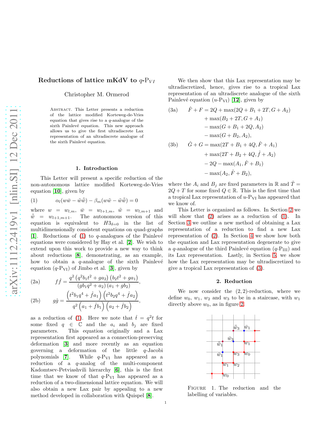
We now consider the (2, 2)-reduction, where we define w 0 , w 1 , w 2 and w 3 to be in a staircase, with w 1 directly above w 0 , as in figure 2. Notice that the evolution is consistent, so long as α l /β m = α l+2 /β m+2 , by which a separation of variables gives us (4)

To satisfy (4), we define constants a i and b i , for i = 1, 2, by letting

If we let t = q m-l , we have that β m /α l ∝ t, where the shift m → m + 2 is equivalent to t → q 2 t. We solve (1) to find w0 and w2 , given by

where we may subsequently use the periodicity and ( 1) to obtain w0 and w2 , given by w1 = w 3 tb 1 w2 q 2 + a 1 w0

Letting w 0 /w 2 = f /t and w 1 /w 3 = g/t gives (2), where we now interpret f and g to be f ĝ respectively.

We use a different approach to reductions to that of Hay et al. [2]. The general method will be further explored in a separate publication [8].

We first note that (1) is multilinear and multidimensionally consistent, giving rise to the following Lax representation

where

and where γ is a spectral parameter [2].

We define two variables,

and a new linear system, φ(x, t), satisfying φ(q 2 x, t) = A(x, t)φ(x, t), (7a) φ(x, q 2 t) = B(x, t)φ(x, t), (7b) where operators A(x, t) and B(x, t) may be interpreted as operating in the (2, 2)-and (0, 2)-directions respectively in our original system. The (2, 2)-operator has the effect of fixing t and letting z → z/q 2 and the (0, 2)-operator fixes z and lets t → q 2 t. We may explicitly construct A(x, t) and B(x, t) in terms of L and M :

where we have directly substituted for x and t. The consistency of (7a) and (7b), which reads (8)

A(x, q 2 t)B(x, t) = B(q 2 x, t)A(x, t), results in (5). We may recast this system by the same identification that related (5) to (2), with an additional factor, h = w 3 , which we interpret to be a gauge factor [3]. Under this identification, we may manipulate the matrices to obtain an equivalent A(x, t) in terms of f , g and h;

where we have used the definitions and ( 5). Note that

and that the leading matrices in the expansion of A(x, t) around x = 0 and x = ∞ are both proportional to the identity matrix, meaning that (7a) and (7b) constitute a connection preserving deformation [3]. The compatibility, given by ( 8), results in (2). However, we obtain a necessary equation satisfied by the gauge factor:

, which bears some similarity to the equation satisfied by the gauge factor of Jimbo et al. [3].

When b 1 = b 2 , the evolution factorizes into two copies of the one mapping, which is also known as q-P III , whose Lax representation was found by Papageorgiou et al. [9]. Here, instead of having m → m + 2, we compute m → m + 1, where

…(Full text truncated)…