Diffusion Adaptation over Networks under Imperfect Information Exchange and Non-stationary Data
Adaptive networks rely on in-network and collaborative processing among distributed agents to deliver enhanced performance in estimation and inference tasks. Information is exchanged among the nodes, usually over noisy links. The combination weights …
Authors: Xiaochuan Zhao, Sheng-Yuan Tu, Ali H. Sayed
1 Dif fusion Adaptation Ov er Netw orks Under Imperfec t Information Exchange and Non-Stationary Dat a Xiaochuan Zhao, Student Member , IEEE, Sheng-Y uan T u, Student Member , IEEE, and Ali H. Sayed, F ellow , IEEE Abstract Adaptive networks rely on in- network and collabo rativ e pro cessing among distributed agents to deliver enhanced perf ormanc e in estimation and infere nce tas ks. In formation is exchanged am ong the nodes, usually over noisy links. The co mbination weights that are u sed by the nod es to fuse inform ation from their n eighbor s play a critical role in in fluencing the ad aptation and tracking abilities of the n etwork. This paper first investigates th e m ean-squar e per forman ce of ge neral ad aptive diffusion algorith ms in the presence of various sources of imperfe ct information exchang es, quantization er rors, and model no n- stationarities. Among other r esults, the a nalysis reveals th at link no ise over the r egression data modifies the dyn amics of the network ev olution in a distinct way , and leads to b iased estimates in steady-state. The ana lysis also re veals how th e n etwork mean-squ are pe rforman ce is dependen t on the comb ination weights. W e use these observations to show how the com bination weights can be optimized and adapte d. Simulation results illu strate the th eoretical findin gs an d match well with the ory . Index T erms Diffusion adaptation, adapti ve networks, imperfect information exchange, tracking behavior, diffusion LMS, comb ination weig hts, energy conservation. The authors are with Department of E lectrical Engineering, Univ ersity of Calif ornia, L os Angeles, CA 90095, Email: { xzhao, shinetu, sayed } @ee.ucla.edu. This work was supported in part by NSF grants CCF-0942936 and CCF-1011918. A short version of t his work was accepted for the IEE E International Conference on Communications (I CC), Ottawa, ON, Canada, June 2012 [1]. September 12, 2018 DRAFT 2 I . I N T R O D U C T I O N A N a daptiv e network consists of a c ollection of agents that are interconne cted to each other a nd solve dis trib uted estimation and inference problems in a collaborati ve manne r . T wo useful str ategies that en able ad aptation and lea rning over suc h networks in real-time are the incremental strategy [2]–[7 ] and the dif fus ion strategy [8]–[12]. Increme ntal strategies rely on the use of a Hamilt onian cycle, i.e., a cyclic pa th that covers a ll nodes in the network, which is ge nerally dif ficult to enforce since d etermining a Hamiltonian cycle is an NP-hard problem. In ad dition, cyclic trajectories a re not robust to node or link failure. In co mparison, d if fusion strategies are scalable, robust, and able to match well the performance of incremental networks. In adap ti ve diff usion implemen tations, information is processe d locally at the nodes and then d if fused in real-ti me across the network. Diffusion s trategies were originally proposed in [8]– [10] a nd further extend ed and studied in [11]–[17]. They have bee n applied to model self-or ganized and complex behavior enc ountered in biological n etworks, suc h as fish s chooling [18], bird flight formations [19], an d bee swarming [20]. Dif fusion strategies have als o been a pplied to on line learning o f Gaussian mixture models [21], [22] and to ge neral distrib uted optimization problems [23]. The re hav e also been several useful w orks in the l iterature on distrib uted consensus-type strategies, with application to multi- agent formations a nd d istrib uted proc essing [24 ]–[31]. The main difference between these works an d the dif fusion approach of [9], [11], [12] is the latter’ s emphasis on the role of ada ptation and learning over networks. In the o riginal d if fusion least-mean-squa res (LMS) strategy [9], [11], the weight estimates that are exchange d a mong the nodes can be subjec t to qu antization errors a nd ad diti ve noise over the c ommu- nication links. Studying the degradation in mea n-square p erformance that results from these particular perturbations can be pu rsued, for both incremental and diffusion strategies, by extending the me an-square analysis already presented in [9], [11 ], in the same manner that the tr acking analysis of con ventional s tand- alone adap ti ve filters was o btained from the counterpa rt results in the stationary case (as explained in [32 , Ch. 2 1]). Useful res ults alon g these lines, which s tudy the effect of link noise during the exchang e of the weight e stimates, alread y appe ar for the traditional dif fusion algorithm in the works [33]–[36] and for consen sus-bas ed algorithms in [37 ], [38]. In this pape r , ou r objec ti ve is to go beyond these earlier studies by taking into a ccount additional ef fects, and by con sidering a more general algorithmic structure. The reason for this le vel of gen erality is be cause the analytical r esults will help re veal wh ich noise sources influence the network performanc e more seriously , in what manne r , a nd at what s tage of the a daptation process . T he results wil l suggest important r emedies and mechan isms to adapt the combination weights September 12, 2018 DRAFT 3 in real-time. Some of these insights are hard t o get if one foc uses solely on n oise during the excha nge of the weigh t estimates. The an alysis will further s how that no ise during the exchan ge of the r egression data plays a more critical role than othe r s ources of impe rfection: this particular no ise alters the learning dynamics and mode s of the n etwork, an d biases the weight estimates . Noises re lated to the excha nge of other pieces of information d o n ot alter the dynamics of the network but contribute to the de terioration of the network performance. T o arrive at these results, i n this p aper , we first consider a g eneralized a nalysis that a pplies to a broad class of dif fusion ad aptation strategies (se e (5)–(7) further ahead ; this cla ss includes the original dif fusion strategi es (3) and (4) as two spec ial cas es). The analysis all ows us t o account for v arious sources of information noise over the co mmunication li nks. W e allow for noisy exc hanges d uring each of the three processing steps of the adapti ve diffusion algorithm (the t wo combination s teps (5) and (7) a nd the adaptation step (6)). In this way , we are able to examine how the three s ets o f combina tion coefficients { a 1 ,lk , c lk , a 2 ,lk } in (5)–(7) influence the propagation of the n oise s ignals throu gh the network dynamics. Our results further re veal how the network mean -square-error p erformance is depende nt on these co mbination weights. Following this line of reasoning, the analysis leads to algorithms (124) and (128 ) further ahead for choos ing the c ombination co efficients to improve the stea dy-state ne twork performance. It s hould be no ted that several c ombination rules, s uch as the Metropolis rule [39] and the maximum degree rule [40] , were propo sed pre viously in the l iterature — esp ecially in the context o f consen sus-base d iterations [40]–[42]. These schemes , howe ver , us ually suffer performanc e degrada tion in the presen ce of noisy information exchange since they ignore the network noise profi le [15]. Wh en the noise variance dif fers ac ross the nod es, it become s ne cessa ry to de sign combination rules that are aware of this variation as outlined further ahea d in Section VI -B. Moreover , in a mobile netw ork [ 18] where nodes are on the move and where neigh borhoods evolve over time, it is even more critical to employ adap ti ve combination strategies that are able to track the variations in the noise profile in orde r to co pe with su ch dyn amic en vironments. This i ssue is taken up in Section VI-C. A. Notation W e u se lowercase letters to d enote vectors, u ppercase letters for matrices, plain letters for deterministic variables, and boldface letters f or random variables. W e a lso use ( · ) ∗ to denote conjuga te transposition, T r( · ) for the trace of its matrix argument, ρ ( · ) for the sp ectral radius of its matri x argument, ⊗ for the Kronecker product, and v ec( · ) for a vector formed by stacking the columns o f i ts matrix a r gument. September 12, 2018 DRAFT 4 W e further use diag {· · · } to denote a (block) dia gonal matrix formed from its arguments, a nd col {· · · } to denote a c olumn vector formed by s tacking its arguments on top of ea ch other . All vectors in our treatment are column vectors , with the exce ption of the regress ion vectors, u k ,i , and the ass ociated no ise signals, v ( u ) lk ,i , wh ich are taken to be row vec tors for co n venie nce of presentation. I I . D I FF U S I O N A L G O R I T H M S W I T H I M P E R F E C T I N F O R M A T I O N E X C H A N G E W e consider a connected n etwork consisting of N n odes. Each node k collects scalar measuremen ts d k ( i ) and 1 × M r egression data vectors u k ,i over success i ve time instants i ≥ 0 . Note that we use parenthesis to refer to the time-dep endenc e o f scalar variables, a s in d k ( i ) , and sub scripts to refer to the time-dependen ce of vector v ariables, as in u k ,i . The mea surements across all node s are assumed to be related to an unkn own M × 1 vector w o via a linear regression model of the form [32]: d k ( i ) = u k ,i w o + v k ( i ) (1) where v k ( i ) deno tes the measurement or model noise with ze ro mean and variance σ 2 v,k . The vector w o in (1) d enotes the parameter o f interest, su ch a s the p arameters o f so me un derlying ph ysical phe nomenon, the taps of a commun ication chann el, or the location o f food sources o r predators. S uch d ata models a re also us eful in s tudies on hybrid combinations of adapti ve fi lters [43]–[47]. The no des in t he network would lik e to estimate w o by solving the follo wing minimization problem: minimize w N X k =1 E | d k ( i ) − u k ,i w | 2 (2) In previous works [9], [11], [13], we introduced an d s tudied several distrib uted strategies of the diff usion type that allow node s to cooperate with each other in order to so lve problems of the form (2) in an adaptive mann er . These diff usion strategies endow networks wit h ad aptation and learning abilities, a nd enable information to diffuse through the network in real-time. W e revie w the ad apti ve dif fusion strategies below . A. Dif fusion Adaptation with P e rfect Information Exchange In [9], [11], two c lasses of dif fusion algorithms were proposed. One c lass is the so-called Combine- then-Adapt (CT A) strategy: φ k ,i − 1 = X l ∈N k a 1 ,lk w l,i − 1 w k ,i = φ k ,i − 1 + µ k X l ∈N k c lk u ∗ l,i [ d l ( i ) − u l,i φ k ,i − 1 ] (3) September 12, 2018 DRAFT 5 and the second class is the so-c alled Adapt-then-Comb ine (A TC) strategy: ψ k ,i = w k ,i − 1 + µ k X l ∈N k c lk u ∗ l,i [ d l ( i ) − u l,i w k ,i − 1 ] w k ,i = X l ∈N k a 2 ,lk ψ l,i (4) where the { µ k } are small positi ve step-size parameters and the { a 1 ,lk , c lk , a 2 ,lk } are nonnegati ve e ntries of the N × N matrices { A 1 , C, A 2 } , resp ectiv ely . The coe f ficients { a 1 ,lk , c lk , a 2 ,lk } are zero whenever node l is not connec ted to nod e k , i.e., l / ∈ N k , where N k denotes the neigh borhood of node k . Th e two strategies (3) a nd (4) c an be inte grated into one broad class o f diffusion ada ptation [11]: φ k ,i − 1 = X l ∈N k a 1 ,lk w l,i − 1 (5) ψ k ,i = φ k ,i − 1 + µ k X l ∈N k c lk u ∗ l,i [ d l ( i ) − u l,i φ k ,i − 1 ] (6) w k ,i = X l ∈N k a 2 ,lk ψ l,i (7) Several diffusion strategies can be obtaine d as special cases o f (5)–(7) throu gh prope r selec tion of the coefficients { a 1 ,lk , c lk , a 2 ,lk } . For examp le, to rec over the CT A strategy (3), we se t A 2 = I N , an d to recover the A TC strategy (4), we set A 1 = I N , where I N denotes the N × N ide ntity ma trix. In the general diff usion s trategy (5)–(7), each no de k ev aluates its estimate w k ,i at time i b y relying s olely on the d ata collected from its neighbors through steps (5) and (7) and on its loc al measu rements through step (6). The matrices A 1 , A 2 , a nd C are required to be left or right-stoch astic, i.e., A T 1 1 N = 1 N , A T 2 1 N = 1 N , C 1 N = 1 N (8) where 1 N denotes the N × 1 vector whos e entries are all one . This mean s that ea ch no de performs a con vex combination o f the e stimates received from its neigh bors at every iteration i . The mean-squa re pe rformance and con ver gence p roperties of the dif fusion a lgorithm (5)–(7) have already be en studied in d etail in [9], [11]. For the ben efit of the an alysis in the subsequ ent s ections, we present below in (21) the recursion describing the ev olution of the weight error vectors a cross the network. T o do so, we introduc e the e rror vectors: e φ k ,i − 1 , w o − φ k ,i − 1 (9) e ψ k ,i , w o − ψ k ,i (10) e w k ,i , w o − w k ,i (11) September 12, 2018 DRAFT 6 and s ubstitute the linea r model (1) into the adaptation step ( 6) to find tha t e ψ k ,i = ( I M − µ k R k ,i ) e φ k ,i − 1 − µ k X l ∈N k c lk s l,i (12) where the M × M matrix R k ,i and the M × 1 vector s k ,i are d efined as : R k ,i , X l ∈N k c lk u ∗ l,i u l,i (13) s k ,i , u ∗ k ,i v k ( i ) (14) W e further collec t the various quantities a cross all nodes in the ne twork into the follo wing bloc k vectors and matrices : R i , diag { R 1 ,i , . . . , R N ,i } (15) s i , col { s 1 ,i , . . . , s N ,i } (16) M , diag { µ 1 I M , . . . , µ N I M } (17) e φ i , col n e φ 1 ,i , . . . , e φ N ,i o (18) e ψ i , col n e ψ 1 ,i , . . . , e ψ N ,i o (19) e w i , col { e w 1 ,i , . . . , e w N ,i } (20) Then, from (5), (7), and (12), the recu rsion for the network error vector e w i is given b y e w i = A T 2 ( I N M − M R i ) A T 1 e w i − 1 − A T 2 MC T s i (21) where A 1 , A 1 ⊗ I M , C , C ⊗ I M , A 2 , A 2 ⊗ I M (22) B. Noisy Infor mation Ex change Each of the steps in (5)–(7) in v olves the sh aring of information between node k and its neighbors. For example, in the first step (5), all neigh bors of node k send the ir e stimates w l,i − 1 to no de k . This transmission is ge nerally subject to ad diti ve noise and possibly quantization errors. Like wise, steps (6) and (7) in volve the sharing o f other pieces of information with node k . These exchange s teps can all be subject to perturbations (such as ad diti ve noise and qu antization errors). One of the objectiv es of this w ork is to analyze the aggr e g ate ef fect of thes e p erturbations on gene ral dif fusion strategies of the type (5)–(7) and to p ropose cho ices for the combination weights in o rder to enha nce the me an-square performance of the network in the presenc e of these disturban ces. September 12, 2018 DRAFT 7 Fig. 1. Sev eral additi ve noise sources perturb the exchang e of information from node l to node k . So let us examine wha t hap pens when information is exch anged over links with ad diti ve noise. W e model the data received by node k from its neighbor l as w lk ,i − 1 , w l,i − 1 + v ( w ) lk ,i − 1 (23) ψ lk ,i , ψ l,i + v ( ψ ) lk ,i (24) d lk ( i ) , d l ( i ) + v ( d ) lk ( i ) (25) u lk ,i , u l,i + v ( u ) lk ,i (26) where v ( w ) lk ,i − 1 and v ( ψ ) lk ,i are M × 1 noise signals, v ( u ) lk ,i is a 1 × M noise signal, and v ( d ) lk ( i ) is a s calar noise signal (see Fig. 1). Ob serve further that in (23)–(26), we are including sev eral source s of information exchange noise. In comparison, referenc es [33]–[35] only conside red the no ise s ource v ( w ) lk ,i − 1 in (23) an d one set of combination coef ficients { a 1 ,lk } ; the other coef ficients were set to c lk = a 2 ,lk = 0 for l 6 = k and c k k = a 2 ,k k = 1 . In o ther words, these references only cons idered (23) and the following traditional CT A s trategy without e xchan ge of the data { d l ( i ) , u l,i } — compare wit h (3); n ote tha t the second s tep in (27) only uses { d k ( i ) , u k ,i } : φ k ,i − 1 = X l ∈N k a 1 ,lk w l,i − 1 w k ,i = φ k ,i − 1 + µ k u ∗ k ,i [ d k ( i ) − u k ,i φ k ,i − 1 ] (27) The a nalysis that follows examines the aggregate eff ect of all four n oise s ources ap pearing in (23)–(26), in add ition to the three sets of c ombination coe f ficients appea ring in (5)–(7). W e introduce the following assumption on the statistical properties of the measurement data and nois e signals. September 12, 2018 DRAFT 8 Assumption 2.1 (Statistical pr operties of the variables): 1) The regression d ata u k ,i are temporally white and s patially indepen dent random variables with zero mean a nd covariance matrix R u,k , E u ∗ k ,i u k ,i ≥ 0 . 2) The no ise signa ls v k ( i ) , v ( w ) lk ,i − 1 , v ( d ) lk ( i ) , v ( u ) lk ,i , a nd v ( ψ ) lk ,i are te mporally white and s patially inde- penden t random variables with zero mean and (co)variances σ 2 v,k , R ( w ) v,l k , σ 2 v,l k , R ( u ) v,l k , an d R ( ψ ) v,l k , respectively . In a ddition, R ( w ) v,l k , σ 2 v,l k , R ( u ) v,l k , a nd R ( ψ ) v,l k are all zero if l / ∈ N k or l = k . 3) The regress ion data { u m,i 1 } , the model noise s ignals { v n ( i 2 ) } , and the link n oise s ignals { v ( w ) l 1 k 1 ,j 1 } , { v ( d ) l 2 k 2 ( j 2 ) } , { v ( u ) l 3 k 3 ,j 3 } , and { v ( ψ ) l 4 k 4 ,j 4 } are mutually-i ndepe ndent random v ariables for all { i 1 , i 2 , j 1 , j 2 , j 3 , j 4 } and { m, n, l 1 , l 2 , l 3 , l 4 , k 1 , k 2 , k 3 , k 4 } . Using the perturbed data (23 )–(26), the dif fusion algorithm (5)–(7) become s φ k ,i − 1 = X l ∈N k a 1 ,lk w lk ,i − 1 (28) ψ k ,i = φ k ,i − 1 + µ k X l ∈N k c lk u ∗ lk ,i [ d lk ( i ) − u lk ,i φ k ,i − 1 ] (29) w k ,i = X l ∈N k a 2 ,lk ψ lk ,i (30) where we continue to use the symbo ls { φ k ,i − 1 , ψ k ,i , w k ,i } to av oid an explosion of no tation. From (23) and (24), expressions (28) –(30) can be re written a s φ k ,i − 1 = X l ∈N k a 1 ,lk w l,i − 1 + v ( w ) k ,i − 1 (31) ψ k ,i = φ k ,i − 1 + µ k X l ∈N k c lk u ∗ lk ,i [ d lk ( i ) − u lk ,i φ k ,i − 1 ] (32) w k ,i = X l ∈N k a 2 ,lk ψ l,i + v ( ψ ) k ,i (33) where we a re introduc ing the symbols v ( w ) k ,i − 1 and v ( ψ ) k ,i to de note the aggregate M × 1 zero-mea n noise signals d efined over the neighborhoo d of node k : v ( w ) k ,i − 1 , X l ∈N k \{ k } a 1 ,lk v ( w ) lk ,i − 1 (34) v ( ψ ) k ,i , X l ∈N k \{ k } a 2 ,lk v ( ψ ) lk ,i (35) September 12, 2018 DRAFT 9 with covariance ma trices R ( w ) v,k , X l ∈N k \{ k } a 2 1 ,lk R ( w ) v,l k (36) R ( ψ ) v,k , X l ∈N k \{ k } a 2 2 ,lk R ( ψ ) v,l k (37) It is worth noting tha t R ( w ) v,k and R ( ψ ) v,k depend on the combination c oefficients { a 1 ,lk } and { a 2 ,lk } , respectively . This prope rty will b e taken into ac count whe n optimizing over { a 1 ,lk } and { a 2 ,lk } in a later se ction. W e furt her introduce the following sca lar zero-mean no ise signa l: v lk ( i ) , v l ( i ) + v ( d ) lk ( i ) − v ( u ) lk ,i w o (38) for l ∈ N k \{ k } , whose variance is σ 2 lk , σ 2 v,l + σ 2 v,l k + w o ∗ R ( u ) v,l k w o (39) T o u nify the notation, we d efine v k k ( i ) , v k ( i ) . T hen, from (1), (25), an d (26), it is e asy to v erify that the n oisy data { d lk ( i ) , u lk ,i } are related via d lk ( i ) = u lk ,i w o + v lk ( i ) (40) for l ∈ N k . Co ntinuing with the adaptation step (32) and s ubstituting (40), we get ψ k ,i = φ k ,i − 1 + µ k X l ∈N k c lk u ∗ lk ,i [ u lk ,i e φ k ,i − 1 + v lk ( i )] (41) Then, we can derive the follo wing error recursion for node k (compare with (12)): e ψ k ,i = I M − µ k R ′ k ,i e φ k ,i − 1 − µ k z k ,i (42) where the M × M matrix R ′ k ,i and the M × 1 v ector z k ,i are defin ed a s (compa re with (13) and (14)): R ′ k ,i , X l ∈N k c lk u ∗ lk ,i u lk ,i (43) z k ,i , X l ∈N k c lk u ∗ lk ,i v lk ( i ) (44) W e further introduce the block vectors and matrices: R ′ i , d iag R ′ 1 ,i , . . . , R ′ N ,i (45) z i , col { z 1 ,i , . . . , z N ,i } (46) v ( w ) i , col n v ( w ) 1 ,i , . . . , v ( w ) N ,i o (47) v ( ψ ) i , col n v ( ψ ) 1 ,i , . . . , v ( ψ ) N ,i o (48) September 12, 2018 DRAFT 10 and the corresponding covariance matrices for v ( w ) i and v ( ψ ) i : R ( w ) v , diag n R ( w ) v, 1 , . . . , R ( w ) v,N o (49) R ( ψ ) v , diag n R ( ψ ) v, 1 , . . . , R ( ψ ) v,N o (50) then, from (31), (33 ), and (42), we arriv e at the follo wing recursion for the network weight e rror vector in the presence of n oisy information exchange: e w i = A T 2 e ψ i − v ( ψ ) i = A T 2 h ( I N M − M R ′ i ) e φ i − 1 − M z i i − v ( ψ ) i = A T 2 h ( I N M − M R ′ i )( A T 1 e w i − 1 − v ( w ) i − 1 ) − M z i i − v ( ψ ) i (51) That is, e w i = A T 2 ( I N M − M R ′ i ) A T 1 e w i − 1 − A T 2 ( I N M − M R ′ i ) v ( w ) i − 1 − A T 2 M z i − v ( ψ ) i (52) Compared to the previous error rec ursion (21), the noise terms in (52) c onsist of three parts: • A T 2 ( I N M − M R ′ i ) v ( w ) i − 1 is contributed b y the noise introduced at the information-exchange step (28) befor e adap tation. • A T 2 M z i is c ontrib uted by the noise intr oduced a t the adaptation step (29). • v ( ψ ) i is c ontrib uted by the noise introduce d at the information-excha nge step ( 30) aft er adaptation. I I I . C O N V E R G E N C E I N T H E M E A N W I T H A B I A S Gi ven the weigh t error rec ursion (52), we are now ready to s tudy the mean con ver gence condition for the d if fusion strategy (28)–(30) in the presenc e of disturbanc es during information exchan ge under Assumption 2.1. T aking expec tations of both sides of (52), we get E e w i = B E e w i − 1 − A T 2 I N M − MR ′ · E v ( w ) i − 1 − A T 2 M · E z i − E v ( ψ ) i (53) where B , A T 2 I N M − MR ′ A T 1 (54) R ′ , E R ′ i = diag R ′ 1 , . . . , R ′ N (55) R ′ k , E R ′ k ,i = X l ∈N k c lk R u,l + R ( u ) v,l k (56) From (34), (35), (47), and (48), it can be verified t hat E v ( w ) i − 1 = E v ( ψ ) i = 0 (57) September 12, 2018 DRAFT 11 whereas, from (44) and As sumption 2.1, we get E z k ,i = E " X l ∈N k c lk ( u l,i + v ( u ) lk ,i ) ∗ ( v l ( i ) + v ( d ) lk ( i ) − v ( u ) lk ,i w o ) # = − X l ∈N k c lk R ( u ) v,l k ! w o (58) Let us define an N M × N M matrix R ( u ) v,c that collects all covariance matrices { R ( u ) v,l k } , k , l = 1 , . . . , N , weighted by the corresp onding combination coefficients { c lk } , such that its ( k , l ) th M × M submatrix is c lk R ( u ) v,l k . Note that R ( u ) v,c itself is not a cov ariance matrix becaus e c k k R ( u ) v,k k = 0 for all k . Then, from (46) an d (58), we a rri ve at z , E z i = −R ( u ) v,c ( 1 N ⊗ w o ) (59) Therefore, us ing (57) and (59), expres sion (53) becomes E e w i = B · E e w i − 1 − A T 2 M z (60) with a driving term due to the presence of z . This dri ving term would disap pear from (60) if there were no noise during the exc hange of the regress ion data. T o gua rantee con vergence of (60), the coe f ficient matrix B must be stable, i.e., ρ ( B ) < 1 . Since A T 1 and A T 2 are right-stochastic matrices, it can be shown that the matrix B i s stable whenever I N M − MR ′ itself is stable (see Appen dix A). This fact leads to an upper bo und on the step-sizes { µ k } to gua rantee the c on ver gence o f E e w i to a stead y-state value, namely , we must ha ve µ k < 2 λ max R ′ k (61) for k = 1 , 2 , . . . , N , where λ max ( · ) denotes the lar gest e igen v alue of its matri x ar gument. Note that the neighborhoo d covariance matrix R ′ k in (56) is related to the combination weights { c lk } . If we further assume tha t C is doubly-stochastic, i.e., C 1 N = 1 N , C T 1 N = 1 N (62) then, by Jensen’ s ineq uality [48], λ max ( R ′ k ) = λ max X l ∈N k c lk ( R u,l + R ( u ) v,l k ) ! ≤ X l ∈N k c lk λ max R u,l + R ( u ) v,l k ≤ max l ∈N k λ max R u,l + R ( u ) v,l k (63) September 12, 2018 DRAFT 12 since (i) λ max ( · ) coincides with t he induced 2 -norm for any p ositi ve semi-definite He rmitian matrix; (ii) matrix norms are con vex functions of their arguments [49]; and (iii) by (62), { c lk } are con vex co mbination coefficients. Thus, we o btain a suf ficient cond ition for the con vergence of (60) in lieu o f (61): µ k < 2 max l ∈N k h λ max R u,l + R ( u ) v,l k i (64) for k = 1 , 2 , . . . , N , w here the uppe r bound for the s tep-size µ k becomes indepe ndent of the combination weights { c lk } . This b ound c an be determined solely from k nowledge o f the covariances of the regression data and the a ssociated noise s ignals tha t are acc essible to node k . It is w orth noting that f or traditional dif fusion algorithms where information is perfectly exch anged, c ondition (64) reduces to µ k < 2 max l ∈N k [ λ max ( R u,l )] (65) for k = 1 , 2 , . . . , N . Comparing (64) with (65), we see tha t the link noise v ( u ) lk ,i over regression data reduces the dynamic range of the step-sizes for mea n stability . Now , under (61), and tak ing the limi t of (60) as i → ∞ , we find that the mean e rror vector will con verge to a steady-state value g : g , lim i →∞ E e w i = − ( I N M − B ) − 1 A T 2 M z (66) I V . M E A N - S Q U A R E C O N V E R G E N C E A N A LY S I S It is well-known that study ing the mean-sq uare con ver gence of a single a daptiv e filter is a c hallenging task, sinc e ad apti ve filters are n onlinear , time-vari ant, and s tochastic sys tems. When a network of adaptive nodes is considered , the complexity of the an alysis is compound ed becaus e the node s now influ ence each other’ s behavior . I n order to make the performance analysis more tractab le, we rely on the en er gy conservation approa ch [32 ], [50], which was used succes sfully in [9], [11 ] to study the mean-squ are performance o f d if fusion s trategies under perfect information exc hange con ditions. That argument allows us to deriv e express ions for the mean-squa re-deviati on (MSD) and the exce ss-mean-squ are-error (EMSE) of the ne twork by a nalyzing h ow ene r gy (measured in terms of error variances) flows through the no des. From rec ursion (52) a nd u nder As sumption 2 .1, we c an ob tain the following we ighted variance relation for the global error v ector e w i : E k e w i k 2 Σ = E k e w i − 1 k 2 Σ ′ + E kA T 2 M z i k 2 Σ − 2 Re { E [ z ∗ i MA 2 Σ A T 2 ( I N M − M R ′ i ) A T 1 e w i − 1 ] } + E kA T 2 ( I N M − M R ′ i ) v ( w ) i − 1 k 2 Σ + E k v ( ψ ) i k 2 Σ (67) September 12, 2018 DRAFT 13 where Σ is a n arbitrary N M × N M positi ve semi-defin ite He rmitian ma trix that we are fr ee to choose. Moreover , the notation k x k 2 Σ stands for the quadratic t erm x ∗ Σ x . The weighting matrix Σ ′ in (67) can be express ed a s Σ ′ = B ∗ Σ B + O ( M 2 ) (68) where B is given by (54) and O ( M 2 ) denotes a term on the order o f M 2 . Evaluating the te rm O ( M 2 ) requires knowledge of higher -order statistics of the regression data and link noises, which are not av ailable under current ass umptions. Howev er , this term bec omes negligible if we introduc e a small step-size assumption. Assumption 4.1 (Small step-size s): Th e step-size s are suf ficiently small, i.e., µ k ≪ 1 , s uch that terms depend ing on higher- order powers of the s tep-sizes can be ignored. Hence, in the seq uel we use the approx imation: Σ ′ ≈ B ∗ Σ B (69) Observe that o n the right-hand s ide (RHS) of relation (67), only the first an d third terms relate to the error vector e w i − 1 . By As sumption 2.1, the error vector e w i − 1 is independent o f z i and R ′ i . Thus, from (59), the third term o n RHS of (67) ca n be e xpresse d as Third term on RHS o f ( 67) = − 2 Re { E [ z ∗ i MA 2 Σ A T 2 ( I N M − M R ′ i ) A T 1 ] · E e w i − 1 } = − 2 Re( z ∗ MA 2 Σ A T 2 A T 1 · E e w i − 1 ) + O ( M 2 ) (70) Since we already showed in the p revious section tha t E e w i con ver ges to a fixed bia s g , q uantity (70) will con ver ge to a fixed value as well whe n i → ∞ . Moreover , un der Assu mption 2. 1, the seco nd, fourth, and fifth terms on RHS of relation (67 ) are all fixed values. T herefore, the con vergence of relation (67) depend s on the be havior of the fi rst term E k e w i − 1 k 2 Σ ′ . Although the weighting ma trix Σ ′ of e w i − 1 is dif ferent from the we ighting matrix Σ o f e w i , it turns out that the e ntries of these two matrices are approximately relate d by a linear eq uation shown a head in (72). Introduce the vector no tation [32]: σ = ve c(Σ) , σ ′ = v ec(Σ ′ ) (71) Then, by using the ide ntity ve c( AB C ) = ( C T ⊗ A ) · vec( B ) , it can be verified from (69) that σ ′ ≈ F · σ (72) September 12, 2018 DRAFT 14 where the N 2 M 2 × N 2 M 2 matrix F is gi ven by F , B T ⊗ B ∗ (73) T o guarantee mea n-square con vergence of the algorithm, the step-sizes should be sufficiently small and selected to ensu re that the matrix F is stable [32], i.e., ρ ( F ) < 1 , which is equiv alent to the earlier condition ρ ( B ) < 1 . Although more spe cific conditions for mean-sq uare stability c an be determined without Assu mption 4.1 [32], it is sufficient for our pu rposes h ere to conclude that the diffusion strategy (28)–(30) is stable in the mean and mean-squ are senses if the s tep-sizes { µ k } satisfy (61) or (64) an d are sufficiently small. V . S T E A DY - S TA T E P E R F O R M A N C E A NA L Y S I S The conc lusion so far i s that sufficiently s mall step-sizes ensu re conv ergence of the diffusion s trategy (28)–(30) in the mean and mean -square senses, even in the presence of exchange n oises over the communication links. Let u s now determine expres sions for the error variances in stea dy-state. W e start from the weighted variance relati on (67). In v ie w of (70), it shows t hat the error variance E k e w i k 2 Σ depend s on the mean error E e w i . W e already determined the value of lim i →∞ E e w i in (66). A. Steady-State V ariance R elation W e continue to use the vector notation (71) and proce ed to evaluate all the terms, except the first on e, on RHS of (67) in the following. For the s econd term, it can be expres sed as Second term on RHS o f (67) = T r( A T 2 MR z MA 2 Σ) = h v ec( A T 2 MR z MA 2 ) i ∗ σ (74) where we used the identity T r( W Σ ) = [v ec( W )] ∗ σ for any Hermitian matrix W , a nd R z denotes the autocorrelation matrix of z i . It is shown in Appendix B that R z is given b y R z , E z i z ∗ i ≈ C T S C + T + z z ∗ (75) where C is defined in (22), z is in (59), a nd {S , T } are two N M × N M p ositi ve semi-definite block diagonal matrices: S , d iag σ 2 v, 1 R u, 1 , . . . , σ 2 v,N R u,N (76) T , diag { T 1 , . . . , T N } (77) T k , X l ∈N k c 2 lk h ( σ 2 v,l + σ 2 v,l k ) R ( u ) v,l k + ( σ 2 v,l k + w o ∗ R ( u ) v,l k w o ) R u,l i (78) September 12, 2018 DRAFT 15 From expres sion (70) and Assu mption 4.1, the thir d term on RHS of (67) is gi ven by Third term on RHS o f (67) ≈ − z ∗ MA 2 Σ A T 2 A T 1 ( E e w i − 1 ) − ( E e w i − 1 ) ∗ A 1 A 2 Σ A T 2 M z = − T r { [ A T 2 A T 1 ( E e w i − 1 ) z ∗ MA 2 + A T 2 M z ( E e w i − 1 ) ∗ A 1 A 2 ]Σ } = − h v ec A T 2 A T 1 ( E e w i − 1 ) z ∗ MA 2 + A T 2 M z ( E e w i − 1 ) ∗ A 1 A 2 i ∗ σ (79) Like wise, the fourth term o n RHS of (67) is approximated by Fourth term on RH S of (67) = h v ec E [ A T 2 ( I N M − M R ′ i ) R ( w ) v ( I N M − M R ′ i ) A 2 ] i ∗ σ ≈ h v ec( A T 2 R ( w ) v A 2 ) i ∗ σ (80) where we are now ignoring terms on the order of M and M 2 . The fifth term on RHS of (67) is given by Fifth term on RHS of (67) = h v ec( R ( ψ ) v ) i ∗ σ (81) Let u s introduce R v , A T 2 R ( w ) v A 2 + R ( ψ ) v + A T 2 M ( T + z z ∗ ) MA 2 (82) Y , −A T 2 A T 1 g z ∗ MA 2 = A T 2 A T 1 ( I N M − B ) − 1 A T 2 M z z ∗ MA 2 (83) At stea dy-state, as i → ∞ , by (66) and (74)–(83), the weighted variance relation (67) becomes lim i →∞ E k e w i k 2 σ ≈ lim i →∞ E k e w i − 1 k 2 F σ + h v ec( A T 2 MC T S C MA 2 + R v + Y + Y ∗ ) i ∗ σ (84) where we are using the compact no tation k x k 2 σ to refer to k x k 2 Σ — doing so allo ws us t o represent Σ ′ by the mo re compact relation F σ on RHS of (84); we shall be using the weighting matrix Σ and its vector representation σ interchan geably for ease of notation (li kewi se, for Σ ′ and σ ′ ). The s teady-state weighted variance relation (84 ) can be rewritten as lim i →∞ E k e w i k 2 ( I N 2 M 2 −F ) σ ≈ h v ec( A T 2 MC T S C MA 2 + R v + Y + Y ∗ ) i ∗ σ (85) where the term A T 2 MC T S C MA 2 is c ontrib uted by the model n oise { v k ( i ) } while the remaining t erms {R v , Y } are contributed by the link noises { v ( w ) lk ,i − 1 , v ( d ) lk ( i ) , v ( u ) lk ,i , v ( ψ ) lk ,i } . Rec all that we a re free to cho ose Σ and, hen ce, σ . Let ( I N 2 M 2 − F ) σ = vec(Ω) , where Ω is an other arbitrary positiv e s emi-definite Hermitian matrix. Then, we a rri ve at the follo w ing theo rem. September 12, 2018 DRAFT 16 Theorem 5.1 (Steady-state weighted va riance relation): Under Assump tions 2.1 and 4.1, for any pos - iti ve semi-definite Hermitian matri x Ω , the steady-state weighted error v ariance relation of the dif fusion strategy (28)–(30) is approximately given by lim i →∞ E k e w i k 2 Ω ≈ h v ec( A T 2 MC T S C MA 2 + R v + Y + Y ∗ ) i ∗ ( I N 2 M 2 − F ) − 1 v ec(Ω) (86) where S is given in (76), R v in (82), Y in ( 83), and F in (73). B. Network MSD a nd EMSE Each subvector of e w i correspond s to the estimation error at a particular node, s ay , e w k ,i for node k . The ne twork MSD is de fined as [ 32]: MSD , lim i →∞ 1 N N X k =1 E k e w k ,i k 2 (87) Since we are free to choose Ω , we select it as Ω = I N M / N . Then, expres sion (86) gives MSD ≈ 1 N h v ec( A T 2 MC T S C MA 2 + R v + Y + Y ∗ ) i ∗ ( I N 2 M 2 − F ) − 1 v ec( I N M ) (88) Similarly , if we instead select Ω = R u / N , where R u , d iag { R u, 1 , . . . , R u,N } (89) then express ion (86) would allow us to evaluate the n etwork EMSE a s: EMSE ≈ 1 N h v ec( A T 2 MC T S C MA 2 + R v + Y + Y ∗ ) i ∗ ( I N 2 M 2 − F ) − 1 v ec( R u ) (90) where, un der Assu mption 2.1, the network E MSE is gi ven by EMSE , lim i →∞ 1 N N X k =1 E | u k ,i e w k ,i − 1 | 2 = lim i →∞ 1 N N X k =1 E k e w k ,i k 2 R u (91) C. Simplifications wh en Regr es sion Da ta are no t Shared W e showed in the earlier sections that the link noise over regression data biase s the weigh t e stimators. In this sec tion we examine how the re sults s implify when there is no sharing o f regress ion data among the n odes. Assumption 5.2 (No sh aring of re gression data): No des do not share regression da ta within neighb or- hoods, i.e., assume C = I N . September 12, 2018 DRAFT 17 By As sumptions 4.1 and 5 .2, matrices {B , R v , Y } in (54), (82), and ( 83) become B = A T 2 ( I N M − MR u ) A T 1 (92) R v = A T 2 R ( w ) v A 2 + R ( ψ ) v (93) Y = 0 (94) where R u is given in (89). Then , the ne twork MSD and EMSE expressions (88) and (90) s implify to: MSD ≈ 1 N h v ec( A T 2 MS MA 2 + R v ) i ∗ ( I N 2 M 2 − F ) − 1 v ec( I N M ) (95) and EMSE ≈ 1 N h v ec( A T 2 MS MA 2 + R v ) i ∗ ( I N 2 M 2 − F ) − 1 v ec( R u ) (96) D. Depend ence of P erforma nce on Combination W eights and Link Noise Recalling that R v and F are related to the combina tion matrices {A 1 , A 2 } , or , equiv alently , { A 1 , A 2 } , results (95) and (96) expres s the network MSD and EMSE in terms of { A 1 , A 2 } . Howev er , it is generally dif ficult to u se the se express ions to o ptimize over { A 1 , A 2 } to red uce the impact of link noise. Instea d, b y substituting (73) into (95) a nd using the fact that F is stable, we can arri ve at ano ther use ful expres sion for the network MSD: MSD ≈ 1 N h v ec( A T 2 MS MA 2 + R v ) i ∗ ∞ X j =0 F j v ec( I N M ) = 1 N h v ec( A T 2 MS MA 2 + R v ) i ∗ ∞ X j =0 ( B T ⊗ B ∗ ) j v ec( I N M ) = 1 N h v ec( A T 2 MS MA 2 + R v ) i ∗ ∞ X j =0 v ec( B ∗ j B j ) (97) That is, MSD ≈ 1 N ∞ X j =0 T r h B j ( A T 2 MS MA 2 + R v ) B ∗ j i (98) where B is gi ven in (92 ). Simil arly , the ne twork EMSE ca n be e xpresse d as EMSE ≈ 1 N ∞ X j =0 T r h B j ( A T 2 MS MA 2 + R v ) B ∗ j R u i (99) September 12, 2018 DRAFT 18 Expression s (98) and (99) reveal in a n interesting way how the noise s ources originating from a ny particular no de end u p influ encing the overall network performanc e. Let u s deno te B i , A T 2 ( I N M − M R ′ i ) A T 1 (100) θ i , A T 2 ( I N M − M R ′ i ) v ( w ) i − 1 + A T 2 M z i + v ( ψ ) i (101) The error recursion (52) c an be re writt en as e w i = B i e w i − 1 − θ i = Φ 0 ,i e w − 1 − i X m =0 Φ m +1 ,i θ m (102) where Φ m,i , B i B i − 1 . . . B m , i ≥ m I N M , i < m (103) Then, E k e w i k 2 = E k Φ 0 ,i e w − 1 k 2 + E i X m =0 Φ m +1 ,i θ m 2 (104) Under Ass umption 5.2, { B i , θ i } in (100) and (10 1) ca n be simpli fied a s B i = A T 2 ( I N M − M R i ) A T 1 (105) θ i = A T 2 ( I N M − M R i ) v ( w ) i − 1 + A T 2 M s i + v ( ψ ) i (106) where { R i , s i } are giv en in (15) a nd (16). By Ass umption 2.1, { B i , θ i } are temporally independ ent for dif ferent i and E B i = B , E θ i = 0 (107) where B is gi ven by ( 92). As i → ∞ , the first term on RHS of (104) be comes First te rm on RHS of (104 ) = lim i →∞ T r E Φ 0 ,i ( E e w − 1 e w ∗ − 1 ) Φ ∗ 0 ,i ( a ) ≈ lim i →∞ T r ( E Φ 0 ,i ) ( E e w − 1 e w ∗ − 1 ) ( E Φ 0 ,i ) ∗ = lim i →∞ T r h B i +1 ( E e w − 1 e w ∗ − 1 ) B ( i +1) ∗ i ( b ) = 0 (108) September 12, 2018 DRAFT 19 where (a) is obtained by approximating the expectation of the product by the p roduct of expectations and (b) is due t o t he stability of B . Therefore, the steady-state value of (104) gi ves lim i →∞ E k e w i k 2 = lim i →∞ i X m =0 E k Φ m +1 ,i θ m k 2 ≈ lim i →∞ i X m =0 T r [( E Φ m +1 ,i ) ( E θ m θ ∗ m ) ( E Φ m +1 ,i ) ∗ ] ( a ) ≈ lim i →∞ i X m =0 T r h B i − m ( A T 2 MS MA 2 + R v ) B ( i − m ) ∗ i ( b ) = lim i →∞ i X j =0 T r h B j ( A T 2 MS MA 2 + R v ) B j ∗ i = ∞ X j =0 T r h B j ( A T 2 MS MA 2 + R v ) B ∗ j i (109) where, by (93) and (10 6), (a) is due to E θ m θ ∗ m ≈ A T 2 ( I N M − MR u ) R ( w ) v ( I N M − MR u ) A 2 + A T 2 MS MA 2 + R ( ψ ) v ≈ A T 2 MS MA 2 + A T 2 R ( w ) v A 2 + R ( ψ ) v = A T 2 MS MA 2 + R v (110) and (b) is simply a chan ge of variable: j = i − m . Since the j th term of the summa tion in (98) or (109 ) is contribut ed by the term E θ i − j θ ∗ i − j , which consists of all the noise sources at time i − j , expres sion (98) sh ows how various sources of n oises a re in volved and ho w they contribute to the network MSD. V I . O P T I M I Z I N G T H E C O M B I NAT I O N M A T R I C E S Before we optimize the c ombination matri ces { A 1 , A 2 } , we first specialize the MSD expression (98) and the EMS E expres sion (99) for the A TC a nd CT A algo rithms. For the A TC a lgorithm, we se t A 1 = I N and A 2 = A , an d for the CT A algorithm, we se t A 1 = A and A 2 = I N . Le t us denote A , A ⊗ I M (111) B atc , A T ( I N M − MR u ) (112) B cta , ( I N M − MR u ) A T (113) September 12, 2018 DRAFT 20 Then, we get MSD atc ≈ 1 N ∞ X j =0 T r h B j atc ( A T MS MA + R ( ψ ) v ) B ∗ j atc i (114) EMSE atc ≈ 1 N ∞ X j =0 T r h B j atc ( A T MS MA + R ( ψ ) v ) B ∗ j atc R u i (115) and MSD cta ≈ 1 N ∞ X j =0 T r h B j cta ( MS M + R ( w ) v ) B ∗ j cta i (116) EMSE cta ≈ 1 N ∞ X j =0 T r h B j cta ( MS M + R ( w ) v ) B ∗ j cta R u i (117) A. An Upper Bound for MSD Minimizing the MSD expression (11 4) or the EMSE expression (115) for the A TC algorithm over left- stochas tic matrices A is generally nontri vial. W e pursue an approximate solution that relies on optimizing an uppe r bound an d performs we ll in practice. Let us us e k X k ∗ to den ote the n uclear norm (als o known as the trace norm, or the Ky Fan n -norm) of matrix X [51], which is defi ned as the sum of the s ingular values of X . Therefore, k X k ∗ = k X ∗ k ∗ for any X and k X k ∗ = T r( X ) when X i s H ermitian and positive semi-definite. Let us also denote k X k b, ∞ as the bloc k ma ximum no rm o f matrix X (see Appendix A). Then, T r h B j atc ( A T MS MA + R ( ψ ) v ) B ∗ j atc i = B j atc ( A T MS MA + R ( ψ ) v ) B ∗ j atc ∗ ≤ kB j atc k ∗ · kA T MS MA + R ( ψ ) v k ∗ · kB ∗ j atc k ∗ ≤ c 2 · kB j atc k 2 b, ∞ · T r( A T MS MA + R ( ψ ) v ) ≤ c 2 · kB atc k 2 j b, ∞ · T r( A T MS MA + R ( ψ ) v ) ≤ c 2 · ( kAk b, ∞ · k I N M − MR u k b, ∞ ) 2 j T r( A T MS MA + R ( ψ ) v ) = c 2 · ρ ( I N M − MR u ) 2 j · T r( A T MS MA + R ( ψ ) v ) (118) where c is so me positi ve scalar such that k X k ∗ ≤ c k X k b, ∞ becaus e k X k ∗ and k X k b, ∞ are sub multi- plicati ve norms and all such norms are equiv a lent [49] . In the last step of (118) we u sed Lemmas A.4 September 12, 2018 DRAFT 21 and A.5 from Appen dix A. Th us, we ca n uppe r bound the network MSD (114) by MSD atc ≤ 1 N ∞ X j =0 c 2 · ρ ( I N M − MR u ) 2 j T r( A T MS MA + R ( ψ ) v ) = c 2 N · T r( A T MS MA + R ( ψ ) v ) 1 − [ ρ ( I N M − MR u )] 2 (119) where the combination matrix A a ppears only in the n umerator . B. Minimizing the Upper Boun d The result (119) motiv ates us to cons ider instea d the problem of minimizing the uppe r b ound, n amely , minimize A T r( A T MS MA + R ( ψ ) v ) sub ject to A T 1 = 1 , a lk ≥ 0 , a lk = 0 if l / ∈ N k (120) Using (50) and (76), the cost func tion in (120) can be expressed as T r( A T MS MA + R ( ψ ) v ) = N X k =1 X l ∈N k a 2 lk h µ 2 l σ 2 v,l T r( R u,l ) + T r( R ( ψ ) v,l k ) i (121) Problem (120) can therefore be decoup led into N separate op timization problems of the form: minimize { a lk , l ∈N k } X l ∈N k a 2 lk h µ 2 l σ 2 v,l T r( R u,l ) + T r( R ( ψ ) v,l k ) i sub ject to X l ∈N k a lk = 1 , a lk ≥ 0 , a lk = 0 if l / ∈ N k (122) for k = 1 , . . . , N . W ith each node l ∈ N k , we associate the follo wing no nnegativ e var iance pr oduct measure: γ 2 lk , µ 2 k σ 2 v,k T r( R u,k ) , l = k µ 2 l σ 2 v,l T r( R u,l ) + T r ( R ( ψ ) v,l k ) , l ∈ N k \{ k } (123) This meas ure incorporates information a bout the link noise covari ances { R ( ψ ) v,l k } . The s olution of (122) is then gi ven by a lk = γ − 2 lk P m ∈N k γ − 2 mk , if l ∈ N k 0 , otherwise ( relati ve variance rule ) (124) W e refer to this co mbination rule as the relati ve variance comb ination rule; it is an extens ion of the rule devised in [52 ] to the cas e of noisy information exchang es. In particular , the definition o f the scalars { γ 2 lk } in (123) is d if ferent and no w depe nds on b oth subs cripts l and k . September 12, 2018 DRAFT 22 Minimizing the EMSE expression (115) for the A TC a lgorithm over left-stocha stic matrices A can be pursued in a similar ma nner by noting that T r h B j atc ( A T MS MA + R ( ψ ) v ) B ∗ j atc R u i ≤ c 2 [ ρ ( I N M − MR u )] 2 j T r( A T MS MA + R ( ψ ) v ) T r( R u ) (125) Thus, minimizing the uppe r bou nd of the network EMSE leads to the same solution (124). Us ing the same argument, we can also show that the same resu lt minimizes the upper bou nd of the n etwork MSD or EMSE for the CT A a lgorithm. C. Adaptive Combination Rule T o ap ply the relati ve v ariance combination rule (124), ea ch node k need s to kno w the variance products, { γ 2 lk } , o f their neighbors, which in gen eral are not available since they require knowledge of the q uantities { σ 2 v,l , T r( R u,l ) , T r( R ( ψ ) v,l k ) } . Therefore, we now propose an ada pti ve combination r ule by us ing d ata tha t are av ailable to the individual nodes. For the A TC algorithm, we firs t note from (24) a nd (29) that E k ψ lk ,i − w l,i − 1 k 2 ≈ µ 2 l σ 2 v,l T r( R u,l ) + T r( R ( ψ ) v,l k ) = γ 2 lk (126) for l ∈ N k \{ k } . Since the algorithm c on ver ges in the mea n a nd me an-squa re s enses under Ass umption 4.1, all the estimates { w k ,i } tend close to w o as i → ∞ . This allo ws us to estimate γ 2 lk for node k by using instantaneous realizations of k ψ lk ,i − w k ,i − 1 k 2 , where we rep lace w l,i − 1 by w k ,i − 1 . Similarly , for node k itself, we can use realizations of k ψ k ,i − w k ,i − 1 k 2 to estimate γ 2 k k . T o unify the no tation, we define ψ k k ,i , ψ k ,i . Le t b γ 2 lk ( i ) de note an estimator for γ 2 lk that is computed by node k at time i . Then, one way t o e v aluate b γ 2 lk ( i ) is through the rec ursion: b γ 2 lk ( i ) = (1 − ν k ) b γ 2 lk ( i − 1) + ν k k ψ lk ,i − w k ,i − 1 k 2 (127) for l ∈ N k , where ν k ∈ (0 , 1) is a forgetti ng f actor that is usua lly c lose to one. In this way , we arriv e at the a daptiv e c ombination rule: a lk ( i ) = [ b γ 2 lk ( i )] − 1 P m ∈N k [ b γ 2 mk ( i )] − 1 , if l ∈ N k 0 , otherwise (128) September 12, 2018 DRAFT 23 V I I . M E A N - S Q UA R E T R A C K I N G B E H A V I O R The dif fus ion strategy (5) –(7) is adaptive in nature. On e of the main benefits o f a daptation (by using constant s tep-sizes) is that it endows networks with tracking abilities when the und erlying weigh t vector w o varies with time. In this s ection we a nalyze how we ll a n ad aptiv e network is ab le to track variations in w o . T o do so, we adop t a random-walk model for w o that is common ly used in the literature to desc ribe the n on-stationarity of t he we ight vector [32]. Assumption 7.1 (Random-walk model): Th e weight vector w o change s ac cording to t he model: w o i = w o i − 1 + η i (129) where { w o i } has a cons tant mean w o for all i , { η i } is an i.i.d. random s equenc e with zero mea n and covari ance matrix R η ; the se quence { η i } is indepe ndent of the initial conditions { w o − 1 , w k , − 1 } and of all regression da ta and noise signals a cross the n etwork for a ll time instants. W e now defin e the e rror vector at node k as e w k ,i , w o i − w k ,i (130) so that the global err or rec ursion (52) for the ne twork is replac ed by e w i = A T 2 ( I N M − M R ′ i ) A T 1 e w i − 1 + A T 2 ( I N M − M R ′ i ) A T 1 ζ i − A T 2 ( I N M − M R ′ i ) v ( w ) i − 1 − A T 2 M z i − v ( ψ ) i (131) where the N M × 1 vector ζ i is de fined as ζ i , col { η i , . . . , η i } = 1 N ⊗ η i (132) A. Con verg ence Co nditions By Assumptions 2.1 and 7.1, it can b e verified that the condition for mea n conv ergence continues t o be ρ ( B ) < 1 , wh ere B is defin ed in (54). In addition, it can also be verified that the error recu rsion (131) con ver ges in t he mea n se nse to the sa me non -zero bias vector g as i n (66). From (131) and und er Assumption 4.1, we can deri ve the weighted vari ance relation: E k e w i k 2 σ ≈ E k e w i − 1 k 2 F σ + E kA T 2 ( I N M − M R ′ i ) A T 1 ζ i k 2 σ − 2 Re { E [ z ∗ i MA 2 Σ A T 2 ( I N M − M R ′ i ) A T 1 e w i − 1 ] } + E kA T 2 ( I N M − M R ′ i ) v ( w ) i − 1 k 2 σ + E kA T 2 M z i k 2 σ + E k v ( ψ ) i k 2 σ (133) September 12, 2018 DRAFT 24 where F is given in (73). If the step -sizes are sufficiently sma ll, then we can assume that the network continues to be mean-squ are stable. B. Steady-State P e rformanc e The stea dy-state performance is affected by the non-stationarity of w o . From Assump tion 4.1, at steady- state, express ion (133) becomes lim i →∞ E k e w i k 2 Ω ≈ [v ec( A T 2 MC T S C MA 2 + A T 2 A T 1 R ζ A 1 A 2 + R v + Y + Y ∗ )] ∗ ( I N 2 M 2 − F ) − 1 v ec(Ω) (134) where S is given in (76), R v in (82), Y in ( 83), F in (73), and R ζ is the cov ariance matrix of ζ i : R ζ , E ζ i ζ ∗ i = ( 1 N 1 T N ) ⊗ R η (135) By (8), (22), and (135) , we get A T 2 A T 1 R ζ A 1 A 2 = ( A T 2 A T 1 1 N 1 T N A 1 A 2 ) ⊗ R η = ( 1 N 1 T N ) ⊗ R η = R ζ (136) Then, following the same a r gument that led to (88), we find that the netw ork MSD is no w given by: MSD trk ≈ 1 N [v ec( A T 2 MC T S C MA 2 + R ζ + R v + Y + Y ∗ )] ∗ ( I N 2 M 2 − F ) − 1 v ec( I N M ) (137) Similarly , the network EMS E is gi ven by: EMSE trk ≈ 1 N [v ec( A T 2 MC T S C MA 2 + R ζ + R v + Y + Y ∗ )] ∗ ( I N 2 M 2 − F ) − 1 v ec( R u ) (138) where R u is define d in (89). Observe that the main diff erence relative to (88) and (90) is the add ition of the term R ζ . Therefore, all the results that were deri ved in t he e arlier section, s uch as (95) and (96), continue to hold by adding R ζ . In particular , if Assu mptions 4. 1 and 5 .2 are ad opted, expressions (137) and (138) can be approximated as MSD trk ≈ 1 N [v ec( A T 2 MS MA 2 + R ζ + R v )] ∗ ( I N 2 M 2 − F ) − 1 v ec( I N M ) (139) and EMSE trk ≈ 1 N [v ec( A T 2 MS MA 2 + R ζ + R v )] ∗ ( I N 2 M 2 − F ) − 1 v ec( R u ) (140) where R v is now given in (93). September 12, 2018 DRAFT 25 Fig. 2. A network topology with N = 20 nodes. V I I I . S I M U L A T I O N R E S U L T S W e s imulate two sc enarios: noisy information exchang es and non-stationary en vironments. W e conside r a c onnected network with N = 20 nodes . The ne twork topology is sho wn in Fig. 2. A. Imperfect Infor mation Ex change The unknown complex parame ter w o of length M = 2 is randomly generated; its value is [0 . 37 50 + j 2 . 08 34 , 0 . 71 74 + j 1 . 4123] . W e ad opt uniform step-size s, { µ k = 0 . 01 } , a nd uniformly white Ga ussian regression data with cov ariance matrices { R u,k = σ 2 u,k I M } , w here { σ 2 u,k } a re sh own in Fig. 3a. The variances of the model noise s, { σ 2 v,k } , are randomly gene rated and shown in Fig. 3b. W e also use white Gaussian link noise signals s uch tha t R ( w ) v,l k = σ 2 w ,lk I M , R ( u ) v,l k = σ 2 u,lk I M , and R ( ψ ) v,l k = σ 2 ψ, lk I M . All link noise vari ances , { σ 2 w ,lk , σ 2 v,l k , σ 2 u,lk , σ 2 ψ, lk } , are randomly generated and i llustrated in Fig. 4 from top to bottom. W e assign the link nu mber by the following proc edure. W e d enote the link from no de l to nod e k as ℓ l,k , whe re l 6 = k . Then , w e c ollect the links { ℓ l,k , l ∈ N k \{ k }} in an asc ending order of l in the list L k (which is a se t with or dered elements ) for each node k . For example, for node k = 2 in Fig. 2, it has 6 links; the ordered links are then co llected in L 2 , { ℓ 5 , 2 , ℓ 6 , 2 , ℓ 7 , 2 , ℓ 13 , 2 , ℓ 15 , 2 , ℓ 20 , 2 } . W e concatena te {L k } in an asc ending order o f k to get the overall list L , {L 1 , L 2 , . . . , L N } . Ev entually , the m th link in the network is given by the m th element in the li st L . W e examine the s implified CT A and A TC algorithms in (3) and (4), namely , no sharing o f d ata a mong nodes (i.e., C = I N ), und er various c ombination rules: (i) the relati ve vari ance rule in (124), (ii) the September 12, 2018 DRAFT 26 Metropolis rule in [39]: a lk = 1 max {|N k | , |N l |} , l ∈ N k \{ k } a lk = 1 − X l ∈N k \{ k } a lk , l = k a lk = 0 , l / ∈ N k (141) where |N k | de notes the degree of node k (including the node itself), (iii ) the uniform weighting rule: a lk = 1 |N k | , l ∈ N k a lk = 0 , l / ∈ N k (142) and (i v) the adaptiv e rule in (128) with { ν k = 0 . 05 } . W e plot the n etwork MSD an d EMSE learning curves for A TC algorithms in Figs. 5a a nd 5c by averaging o ver 5 0 experiments. For CT A algorithms, we plot their ne twork MSD and EMSE learning curves in Figs. 5b and 5 d a lso b y averaging over 50 experiments. Moreover , we also plot their theoretica l results (95) an d (96) in the same figu res. From Fig. 5 we see tha t the relati ve v ariance rule makes dif fusion algorithms achiev e the l owest MSD an d EMSE lev els at steady-state, compared to the metr opolis and uniform rules as well as the algorithm from [33] (which also requires k nowledge of the noise variances). In ad dition, the ad aptiv e rule attains MSD and EMSE levels that are only slightly lar ge r than those o f the relative variance rule, a lthough, as e xpected , it c on ver g es s lower due to the additional learning step (127). B. Non-stationary S cenario The value for ea ch entry of the complex parameter w o i = col { w o i, 1 , w o i, 2 } is assumed to be changing over time along a circular trajectory in the complex plane, a s s hown in Fig. 6. The dyna mic mod el for w o i is expressed as w o i,m = e j ω w o i − 1 ,m , where m = 1 , 2 , ω = 2 π / 600 0 , an d w o − 1 = col { 1 + j, − 1 − j } . The cov ariance matrices { R u,k } are ran domly generated such that R u,k 6 = R u,l when k 6 = l , but their traces are no rmalized to be o ne, i.e., T r( R u,k ) = 1 , for all nodes. The variances for the mode l noises, { σ 2 v,k } , are a lso rand omly gene rated. W e examine two different s cenarios: the low noise-level cas e where the average noise variance across the n etwork is − 5 dB an d the noise vari ances are shown in Fig. 7a; a nd the high n oise-lev el case where the average variance is 25 dB an d the variances are shown in F ig. 7b. W e simulate 3000 iterations and av erage over 2 0 experiments in Figs. 6a and 6b for each case . The step-size is 0. 01 a nd un iform ac ross the network. For simplicity , we adopt the simplified A T C algo rithm whe re C = I N , and only use the uniform weighting rule (14 2). The tracking behavior of the ne twork, d enoted September 12, 2018 DRAFT 27 (a) The variance profile of regression data. (b) The varian ce profile of measurement noises. Fig. 3. The v ariance profiles for regression data and measurement noises. Fig. 4. The v ariance profiles for va rious sources of link noises, including { σ 2 w,lk , σ 2 v,lk , σ 2 u,lk , σ 2 ψ ,lk } . as ¯ w i = col { ¯ w i, 1 , ¯ w i, 2 } , is ob tained by averaging over all the es timates, { w k ,i } , across the n etwork. Figs. 6a and 6b de pict the complex plane; the horizontal axis is t he real ax is a nd the vertical axis is the imaginary axis. Therefore, for ev ery time i , each entry of w o i or ¯ w i represents a point in the plan e. Whe n September 12, 2018 DRAFT 28 (a) Network MSD curves for A TC algorithms (b) Network MSD curves for CT A algorithms (c) Network EMSE curves for A TC algorithms (d) Network EMSE curves for CT A algorithms Fig. 5. Simulated network MSD and EMSE curves and t heoretical results (95) and (96) for diffusion algorithms wit h v arious combination rules under noisy information excha nge. i is increasing, w o i, 1 moves along the red trajectory (in ◦ ), w o i, 2 along the blue trajectory (in ), ¯ w i, 1 along the green trajectory (in + ), and ¯ w i, 2 along the magenta trajectory (in × ). From Fig. 6, it can be seen tha t diff usion algorithms exhibit the trac king ab ility in b oth high a nd low noise-level en vironments. I X . C O N C L U S I O N S In this work we in vestigated the performance of dif fusion algorithms under sev eral sources o f noise during information exchange and und er non -stationary en vironments. W e fi rst s howed that, o n one hand, the link no ise over the regression data bia ses the estimators an d deteriorates the c onditions for mea n a nd mean-squa re conv ergence. On the other hand , diffusion strategies c an s till stabilize the mean an d mean- square con vergence of the network with noisy informati on exchange. W e deri ved analytical expressions September 12, 2018 DRAFT 29 (a) The low noise-le vel case. (b) The high noise-lev el case. Fig. 6. An adapti ve network tracking a parameter vecto r w o ∈ C 2 . for the network MSD a nd EMSE and used these expressions to motiv ate the choice of combination weights that he lp ame liorate the e f fect of information-exchan ge n oise a nd improve network pe rformance. W e als o extended the results to the non-stationa ry s cenario where the un known parameter w o is chan ging over time. Simulation results illustrate the theoretical findings and h ow well they match with theory . A P P E N D I X A S TA B I L I T Y O F A T 2 ( I N M − MR ′ ) A T 1 Follo wing [15], we first de fine the bloc k maximum norm of a vector . September 12, 2018 DRAFT 30 (a) The variance profile for low noise-le vel. (b) The variance profile for high noise-lev el. Fig. 7. The noise variance profiles for two cases. Definition A.1 (Block Maximum Norm): Given a vector x = col { x 1 , . . . , x N } ∈ C M N consisting of N bloc ks { x k ∈ C M , k = 1 , . . . , N } , the block maximum norm is the real func tion k · k b, ∞ : C M N → R , defined a s k x k b, ∞ , max 1 ≤ k ≤ N k x k k 2 (143) where k · k 2 denotes the standard 2 -norm on C M . Similarly , we define the matrix norm that is i nduce d by the block maximum no rm as foll ows: Definition A.2 (Block Maximum Matrix Norm): Given a bloc k matrix A ∈ C M N × M N with block s ize M × M , then kAk b, ∞ , max x ∈ C M N \{ 0 } kA x k b, ∞ k x k b, ∞ (144) denotes the induced block max imum (matrix) norm on C M N × M N . Lemma A.3 : The block ma ximum matrix norm is block unitary i n v ariant, i.e., given a block diag onal unitary ma trix U , diag { U 1 , . . . , U N } ∈ C M N × M N consisting of N unitary blocks { U k ∈ C M × M , k = 1 , . . . , N } , where U k U ∗ k = U ∗ k U k = I M , for any ma trix A ∈ C M N × M N , the n kAk b, ∞ = k U A U ∗ k b, ∞ (145) where k · k b, ∞ denotes the block maximum matri x n orm on C M N × M N with block size M × M . September 12, 2018 DRAFT 31 Lemma A.4 : Let A ∈ C N × N be a ri ght-stochas tic matrix. Then, for block size M × M , k A ⊗ I M k b, ∞ = 1 (146) Pr oof: From Defin ition A.2, we get k A ⊗ I M k b, ∞ = max x ∈ C M N \{ 0 } max l k P N k =1 [ A ] lk x k k 2 max k k x k k 2 ≤ max x ∈ C M N \{ 0 } max l P N k =1 [ A ] lk k x k k 2 max k k x k k 2 ≤ max x ∈ C M N \{ 0 } max l ( P N k =1 [ A ] lk ) · max k k x k k 2 max k k x k k 2 ≤ max x ∈ C M N \{ 0 } max l 1 · max k k x k k 2 max k k x k k 2 = 1 (147) where x , col { x 1 , . . . , x N } ∈ C M N consists of N blocks { x k ∈ C M , k = 1 , . . . , N } , and [ A ] lk denotes the ( l, k ) th entry of A . On the o ther han d, for any indu ced matrix no rm, say , the block maximum norm, it is alw ays lower bound ed by the spe ctral radius of the matrix [49 ]: k A ⊗ I M k b, ∞ ≥ ρ ( A ⊗ I M ) = ρ ( A ) = 1 (148) Combining (147) and (148) c ompletes the proof. Lemma A.5 : Let A ∈ C N M × N M be a block diagona l Hermitian matrix with block size M × M . Th en the b lock maximum norm of the matri x A is e qual to its spectral radius , i.e., kAk b, ∞ = ρ ( A ) (149) Pr oof: De note the k th M × M sub matrix o n the diagonal o f A b y A k . Let A k = U k Λ k U ∗ k be the eigen-deco mposition of A k , whe re U k ∈ C M × M is unitary and Λ k ∈ R M × M is diagona l. Define the block unitary matrix U , diag { U 1 , . . . , U N } a nd the diagonal matrix Λ , diag { Λ 1 , . . . , Λ N } . Then , September 12, 2018 DRAFT 32 A = U Λ U ∗ . By Lemma A.3, the block maximum norm of A with block size M × M is kAk b, ∞ = kU Λ U ∗ k b, ∞ = k Λ k b, ∞ = max x ∈ C M N \{ 0 } max k k Λ k x k k 2 max k k x k k 2 ≤ max x ∈ C M N \{ 0 } max k k Λ k k 2 · k x k k 2 max k k x k k 2 ≤ max x ∈ C M N \{ 0 } max k k Λ k k 2 · max k k x k k 2 max k k x k k 2 = max k k Λ k k 2 = ρ ( A ) (150) where we used the fact that the induce d 2 -norm is identical to the s pectral radius for Hermitian matrices [49]. On the other hand, any ma trix no rm is lo wer bounded b y the s pectral radius [49], i.e., ρ ( A ) ≤ kAk b, ∞ (151) Combining (150) and (151) c ompletes the proof. Now we show that the matrix A T 2 ( I N M − MR ′ ) A T 1 is stable if I N M − MR ′ is stable. For any indu ced matrix norm, say , the bloc k maximum n orm with block size M × M , we ha ve [49] ρ A T 2 ( I N M − MR ′ ) A T 1 ≤ kA T 2 ( I N M − MR ′ ) A T 1 k b, ∞ ≤ kA T 2 k b, ∞ · k I N M − MR ′ k b, ∞ · kA T 1 k b, ∞ = k I N M − MR ′ k b, ∞ (152) where, from (8) and (22), A T 1 and A T 2 satisfy Lemma A.4. By (17) and (55), it is straightforward to se e that I N M − MR ′ is bloc k d iagonal with block size M × M . Then, b y Lemma A.5, express ion (152) can b e further expres sed as ρ A T 2 ( I N M − MR ′ ) A T 1 ≤ ρ ( I N M − MR ′ ) (153) which co mpletes the proof. 1 1 This statement fixes the argu ment t hat appeared in Appen dix I of [11] and Lemma 2 of [12 ]. Si nce the matrix X in Appendix I of [11] and the matrix M in Lemma 2 of [12] are block diagonal, the k · k ρ norm used in these references should simply be replaced by the k · k b, ∞ norm used here and as already done in [15]. September 12, 2018 DRAFT 33 A P P E N D I X B P R O O F O F E X P R E S S I O N (75) Let us d enote the ( l , k ) th submatrix of R z by R z ,l k ∈ C M × M . By Ass umptions 2.1 and expression (44), R z ,l k can be e valuated as R z ,l k = E z l,i z ∗ k ,i = X m ∈N l X n ∈N k c ml c nk E u ∗ ml,i v ml ( i ) v ∗ nk ( i ) u nk ,i | {z } , R ml,nk (154) where, by expressions (26 ) and (38), R ml,nk = E u m,i + v ( u ) ml,i ∗ v m ( i ) + v ( d ) ml ( i ) − v ( u ) ml,i w o v n ( i ) + v ( d ) nk ( i ) − v ( u ) nk ,i w o ∗ u n,i + v ( u ) nk ,i (155) When m 6 = n , e xpression (155) reduces to R ml,nk = R ( u ) v,ml w o w o ∗ R ( u ) v,n k (156) When m = n , e xpression (155) becomes R ml,nk = E v m ( i ) + v ( d ) ml ( i ) − v ( u ) ml,i w o v m ( i ) + v ( d ) mk ( i ) − v ( u ) mk, i w o ∗ u m,i + v ( u ) ml,i ∗ u m,i + v ( u ) mk, i = E v m ( i ) + v ( d ) ml ( i ) v m ( i ) + v ( d ) mk ( i ) ∗ E u m,i + v ( u ) ml,i ∗ u m,i + v ( u ) mk, i + E v ( u ) ml,i w o w o ∗ v ( u ) ∗ mk, i u m,i + v ( u ) ml,i ∗ u m,i + v ( u ) mk, i = σ 2 v,m + δ lk σ 2 v,ml R u,m + δ lk R ( u ) v,ml + δ lk w o ∗ R ( u ) v,ml w o R u,m + R ( u ) v,ml w o w o ∗ R ( u ) v,mk + δ lk E v ( u ) ∗ ml,i v ( u ) ml,i w o w o ∗ v ( u ) ∗ ml,i v ( u ) ml,i − R ( u ) v,ml w o w o ∗ R ( u ) v,ml (157) where δ lk denotes the Kronecker delta function. Evaluating the last term on R HS of (157) requires knowledge of the exce ss kurtosis of v ( u ) ml,i , which is gen erally not av ailable. In order to proc eed, we in voke a separation principle to approximate it a s E v ( u ) ∗ ml,i v ( u ) ml,i w o w o ∗ v ( u ) ∗ ml,i v ( u ) ml,i ≈ R ( u ) v,ml w o w o ∗ R ( u ) v,ml (158) Substituting (15 8) into (15 7) leads to R ml,nk ≈ σ 2 v,m + δ lk σ 2 v,ml R u,m + δ lk R ( u ) v,ml + δ lk w o ∗ R ( u ) v,ml w o R u,m + R ( u ) v,ml w o w o ∗ R ( u ) v,mk = σ 2 v,m R u,m + R ( u ) v,ml w o w o ∗ R ( u ) v,mk + δ lk h ( σ 2 v,ml + w o ∗ R ( u ) v,ml w o ) R u,m + ( σ 2 v,m + σ 2 v,ml ) R ( u ) v,ml i (159) September 12, 2018 DRAFT 34 From (156) and (159), w e ge t R ml,nk ≈ R ( u ) v,ml w o w o ∗ R ( u ) v,mk + δ mn σ 2 v,m R u,m + δ mn δ lk h ( σ 2 v,ml + w o ∗ R ( u ) v,ml w o ) R u,m + ( σ 2 v,m + σ 2 v,ml ) R ( u ) v,ml i (160) Substituting (16 0) into (15 4), we obtain R z ,l k ≈ X m ∈N l c ml R ( u ) v,ml w o ! X n ∈N k c nk R ( u ) v,mk w o ! ∗ + X m ∈N l X n ∈N k c ml c nk δ mn σ 2 v,m R u,m + δ lk X m ∈N l c 2 ml h ( σ 2 v,ml + w o ∗ R ( u ) v,ml w o ) R u,m + ( σ 2 v,m + σ 2 v,ml ) R ( u ) v,ml i (161) From (58)–(59) and (76)–(78), we arri ve at expres sion (75). R E F E R E N C E S [1] X. Z hao and A. H. Sayed, “Combination weights for diffusion strategies wit h imperfect information exchange, ” in Proc . IEEE Int. Conf. Commun. (IC C) , Ottawa, Canada, June 2012. [2] J. Tsitsiklis and M. Athans, “Con ve rgence and asy mptotic agreement in distrib uted decision problems, ” IE EE Tr ans. Autom. Contr ol , vol. 29, no. 1, pp. 42–50, Jan. 1984. [3] J. Tsitsiklis, D. Bertsekas, and M. At hans, “Distri buted asynchronous deterministic and st ochastic gradient optimization algorithms, ” IEEE T rans. Autom. Contr ol , vol. 31, no. 9, pp. 803–812, Sept. 1986. [4] D. P . Bertsekas, “ A new class of incremental gradient methods for l east squares problems, ” SIA M J. Optim. , vol. 7, no. 4, pp. 913–926, 1997. [5] A. Nedic and D. P . Bertsekas, “Incremental subgradient methods for nondif ferentiable optimization, ” SIAM J. Optim. , vol. 12, no. 1, pp. 109–138 , 2001. [6] M. G. Rabbat and R . D. No wak, “Quantized incremental algo rithms for distributed optimization, ” IEEE J. Sel. Areas Commun. , vol. 23, no. 4, pp. 798–80 8, Apr . 2005. [7] C. G. Lopes and A. H. Sayed, “Incremental adaptiv e strategies over distributed networks, ” IEE E T rans. Signal Pr ocess. , vol. 48, no. 8, pp. 223–229, Aug. 2007. [8] C. G. Lopes and A . H. Sayed, “Distributed processing ov er adaptiv e networks, ” in Pr oc. Adapt. Sensor Array P r ocess. W orkshop (ASAP ) , MIT Lincoln Laboratory , MA, June 2006, pp. 1–5. [9] C. G. Lopes and A. H. Sayed, “Diffus ion least-mean squares ov er adaptiv e networks: F ormulation and performance analysis, ” IEEE T rans. Signal P r ocess. , vol. 56, no. 7, pp. 3122–313 6, July 2008. [10] F . S. Catt iv elli and A. H. S ayed, “Diffusion LMS algorithms with i nformation exchange, ” in Pr oc. A silomar Conf. Signals, Systems, Computers , Pacific Grov e, CA, Oct. 2008, pp. 251–255. [11] F . S. C attiv elli and A. H. Sayed, “Dif fusion LMS st rategies for distributed estimati on, ” IEEE T ran s. Signal P r ocess. , vol. 58, no. 3, pp. 1035–10 48, Mar . 2010. [12] F . S. Cat tiv elli and A. H. Sayed, “Diffusion str ategies for distributed Kalman filtering and smoothing, ” IEEE Tr ans. Autom. Contr ol , vol. 55, no. 9, pp. 2069–2084, Sept. 2010. [13] F . S. Cattivelli, C. G. Lopes, and A. H. Sayed, “Diffusion recursiv e least-squares for distributed estimation ov er adaptiv e networks, ” IE EE T rans. Signal Proce ss. , vol. 56, no. 5, pp. 1865–1877 , May 2008. September 12, 2018 DRAFT 35 [14] L. L i and J. A. C hambers, “Dist ributed adaptiv e estimation ba sed on t he AP A algorithm over diffusion netowrks with changing topology , ” in Proc. IEEE W orkshop Stat. Signal Pr ocess. (SSP) , Cardiff, UK, A ug. / Sept. 2009, pp. 757–760 . [15] N. T akahashi, I. Y amada, and A. H. Sayed, “Diffusion least-mean squares with adaptiv e combiners: F ormulation and performance analysis, ” IEE E T rans. Signal Proc ess. , vol. 58, no. 9, pp. 4795–4810, Sept. 2010. [16] N. T akahashi and I. Y amada, “Link probability control for probabilistic dif fusion least-mean squares ove r resource- constrained networks, ” i n Pr oc. IEEE Int. Conf. Acoust., Speech, Signal Proc ess. (ICA SSP) , Dallas, TX, Mar . 2010, pp. 3518–3 521. [17] S. Chouva rdas, K. Slavak is, and S. Theodoridis, “ Adaptive robu st distributed learning in dif fusion sensor networks, ” IE EE T rans. Signal Process . , vol. 59, no. 10, pp. 4692–470 7, Oct. 2011. [18] S-Y . Tu and A. H. Sayed, “Mobile adaptiv e networks, ” IE EE J . Sel. T op. Signal Pr ocess. , vol. 5, no. 4, pp. 649–664, Aug. 2011. [19] F . S. Catti velli and A. H. S ayed, “Modeling bird flight formations using diffusion adaptation, ” IEEE Tr ans. Signal Process. , vol. 59, no. 5, pp. 2038–2051, May 2011. [20] J. Li and A. H. Saye d, “Modeling bee swarming behavior through diffusion adaptation with asym metric information sharing, ” EURASIP J. A dvances Signal Proce ss. , pp. 1–14, doi:10.1186/1687–6 180–2012–18, Jan. 2012. [21] Z. T owfic, J. Chen, and A. H. Sayed, “Collaborati ve learn ing of mixture mod els using diffusion adaptation, ” in Proc. IEEE Int. W orkshop Machine Learn. Signal Proc ess. (MLSP) , B eijing, China, Sept. 2011, pp. 1–6. [22] Y . W eng, W . Xi ao, and L. Xie, “Diffusion-b ased EM algorithm for distributed estimation of Gaussian mixtures in wireless sensor networks, ” Senso rs , vol. 11, no. 6, pp. 6297–6316, June 2011. [23] J. Chen and A. H. Sayed, “Diffusion adaptation strategies for distributed optimization and learning ov er networks, ” to appear i n IE EE Tr ans. Signal Pr ocess. , 2012. [Also av ailable online at http://arxiv .org/abs/111 1.0034 as [math.OC] , Oct. 2011.] [24] A. Jad babaie, J. Lin, and A. S. M orse, “Coordination of groups o f mobile autonomou s agents using nearest neighbor rules, ” IEEE T ran s. Autom. Contr ol , vol. 48, no. 6, pp. 988–1001, June 2003. [25] J. A. Fax and R. M. Murray , “Information flo w an d coope rativ e control o f v ehicle formation s, ” IE EE T rans. Autom. Contr ol , vol. 49, no. 9, pp. 1465–1476, Sept. 2004. [26] R. Olfati-Saber , “F locking for multi-agent dynamic systems: Algorithms and t heory , ” IE EE Tr ans. Autom. C ontr ol , vo l. 51, no. 3, pp. 401–420 , Mar . 2006. [27] R. Olfati-Saber and R. M. Murray , “Consensus problems in networks of agents wi th switching topology and time-delays, ” IEEE T ran s. Autom. Contr ol , vol. 49, no. 9, pp. 1520–1533, S ept. 2004. [28] S. Barbarossa and G. Scutari, “Bio-inspired sensor neto wrk design , ” IEEE Signal Pro cess. Mag . , v ol. 24, no. 3, pp. 26–35, May 2007. [29] A. Nedic and A. Ozdaglar , “Distributed subgradient methods for multi-agent optimization, ” IEEE T rans. Signal Pr ocess. , vol. 54, no. 1, pp. 48–61, Jan. 2009. [30] A. G. Dimakis, S. Kar , J. M. F . Moura, M. G. Rabbat, and A. S caglione, “Gossip algorithms for distributed signal processing, ” Pr oc. IEEE , vol. 98, no. 11, pp. 1847–1864, Nov . 2010. [31] S. Kar and J. M. F . Moura, “Conv erg ence rate analysis of distri buted gossip (l inear parameter) estimation: F undamental limits and tradeoffs, ” IEEE J . Sel. T op. Signal Pr ocess. , vol. 5, no. 4, pp. 674–690, Aug. 2011. [32] A. H. Sayed, Adaptive F ilters , Wiley , N J, 2008. September 12, 2018 DRAFT 36 [33] R. Abdolee and B. Champagne , “Diffu sion LMS algorithms for sensor netwo rks ov er non-ideal inter-sensor wireless channels, ” in Pr oc. IEEE Int. Conf. Dist. Comput. Sensor Systems (DCOSS) , Barcelona, Spain, June 2011, pp. 1–6. [34] A. Khalili, M. A. Tinati, A. Rastega rnia, and J. A. Chambers, “Transient analysis of dif fusion least-mean squares adaptiv e networks wi th noisy channels, ” Int. J . Adapt. Contro l Signal Pr ocess. , Sept. 2011, doi: 10.1002/acs.1279. [35] A. Khalili, M. A. T inati, A. Rastegarnia, and J. A. Chambers, “Steady-state analysis of diffusion LMS adaptiv e networks with noisy links, ” IEEE Tr ans. Signal Pr ocess. , vol. 60, no. 2, pp. 974–979, Feb. 2012. [36] S-Y . Tu and A. H. S ayed, “ Adapti ve networks with noisy links, ” in Proc. IEEE Global Commun. Conf. (GLOBE COM) , Houston, TX, Dec. 2011, pp. 1–5. [37] S. Kar and J. M. F . Moura, “Distri buted consensus algorithms in sensor networks: Link failures and channel noise, ” IEEE T rans. Signal Process . , vol. 57, no. 1, pp. 355–369, Jan. 2009. [38] G. Mateos, I. D. S chizas, and G. B . Giannak is, “P erformance analysis of the consensus-based distributed LMS algorithm, ” EURASIP J. Advances Signal Pro cess. , pp. 1–19, Article ID 981030, doi:10.1155/2009 /981030, 2009. [39] N. Metropolis, A. W . Rosenbluth, M. N. Rosenbluth, A. H. T eller, and E . T eller, “Equations of state calculations by fast computing machines, ” J. C hem. Phys. , vol. 21, no. 6, pp. 1087–10 92, 1953. [40] L. Xiao, S. Boyd , an d S. Lall, “ A scheme for robu st distr ibuted sensor fusion based on av erage consensus, ” in Pro c. ACM/IEEE Int. Conf. Inform. Pr ocess. Sensor N etworks (IPSN) , Los Angeles, CA, Apr . 2005, pp. 63–70. [41] L. Xiao and S. Boyd, “Fast linear iterations for distributed averaging, ” System Contr ol Lett. , vol. 53, no. 9, pp. 65–78, Sept. 2004. [42] D. Jakov etic, J. Xavier , and J. M. F . Moura, “W eight optimization for conse nsus algorithms with correlated switching topology , ” IEEE T rans. Signal Process. , vol. 58, no. 7, pp. 3788–3801 , July 2010. [43] J. Ar enas-Garcia, V . Gomez-V erdejo, and A. R. F igueiras-V idal, “New algorithms for improved adapti ve con v ex combination of LMS t ransv ersal fi lters, ” IEEE T ra ns. Instrum. Meas. , vol. 54, no. 6, pp. 2239–224 9, Dec. 2005. [44] D. Mandic, P . V ayanos, C. B oukis, B. Jelfs, S. L. Goh, T . Gautama, and T . Rutko wski, “Collaborativ e adaptiv e learning using hybrid filters, ” in Pr oc. IE EE Int. Conf. Acoust., Speech, Signal Process . (ICASSP) , Honolulu, HI, Apr . 2007, pp. 921–92 4. [45] M. T . M. Silv a and V . H. Nascimen to, “ Improving the tracking capability of adaptiv e fi lters via con vex combination, ” IEEE T ran s. Signal Process . , vol. 56, no. 7, pp. 3137–3149 , July 2008. [46] S. S. K ozat and A. C. S inger , “ A performance-weighted mixture of LMS fi lters, ” in P r oc. IEE E Int. Conf. Acoust., Speech, Signal Pr ocess. (ICASSP) , T aipei, Apr . 2009, pp. 3101–3104. [47] R. Candido, M. T . M. S ilva, and V . H. N ascimento, “Transient and steady-state analysis of the affine combination of two adapti ve filters, ” IEEE Tr ans. Signal Pr ocess. , vol. 58, no. 8, pp. 4064–4078 , Aug. 2010. [48] S. Boyd and L . V andenberghe, Con ve x Optimization , Cambridge Univ . Press, 2004. [49] R. A. Horn and C. R. Johnson, Matrix Analysis , Cambridge Univ . Press, Cambridge, UK, 1985. [50] T . Y . Al-Naffouri and A. H. S ayed, “T ransient analysis of data-normalized adapti ve fi lters, ” IEEE T ran s. Signal P r ocess. , vol. 51, no. 3, pp. 639–652, Mar . 2003. [51] A. J. L aub, Matrix Analysis for Scientists and Engineer s , SIAM, P A, 2005. [52] S-Y . Tu and A. H. Sayed, “Optimal combination rules for adaptation and learning over neto wrks, ” in Proc. IEEE Int. W orkshop Comput. Advances Multi-Sensor Adapt. Process. (CAMSAP) , S an Juan, Puerto Rico, Dec. 2011, pp. 317–320. September 12, 2018 DRAFT
Original Paper
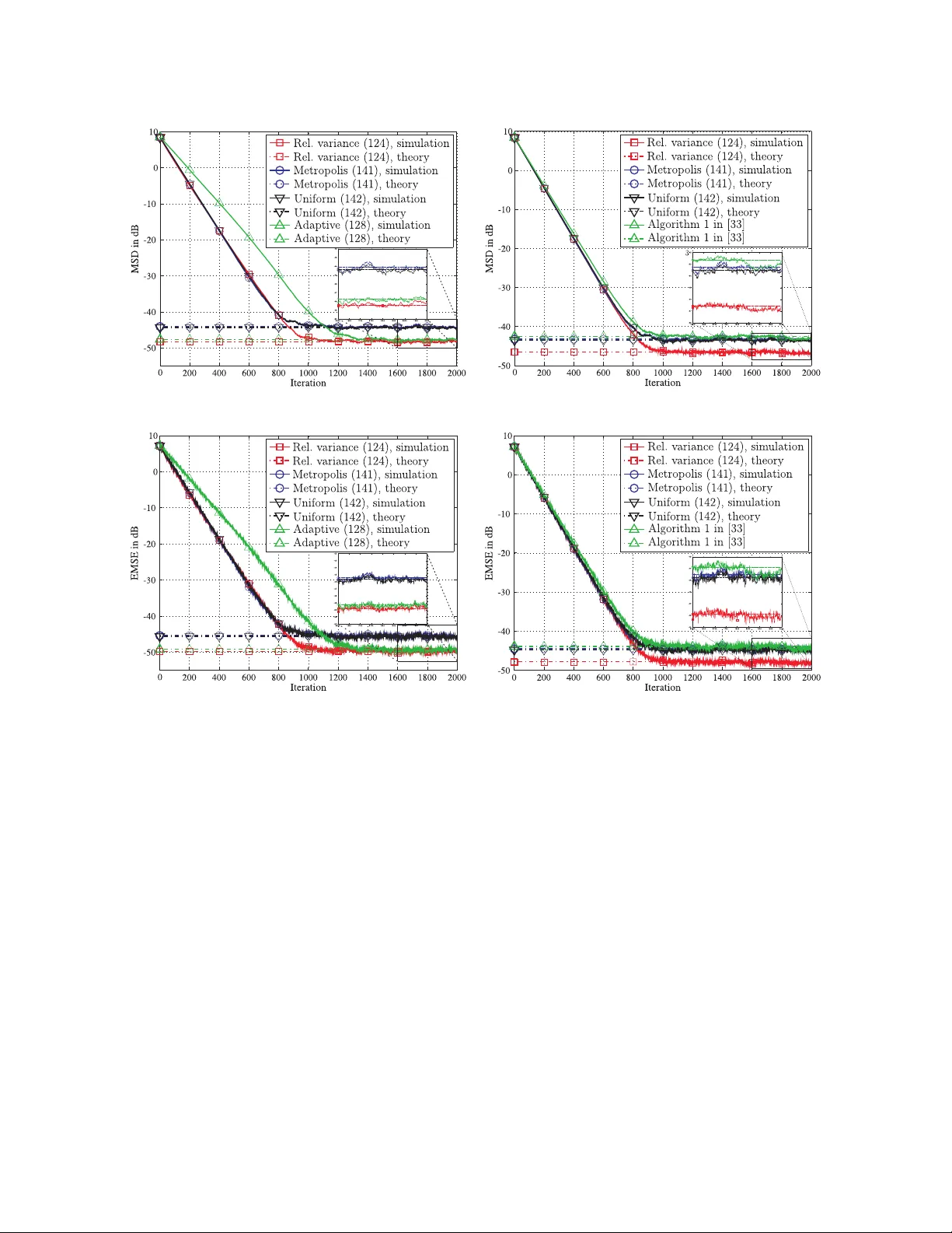
Loading high-quality paper...
Comments & Academic Discussion
Loading comments...
Leave a Comment