Nanohertz Frequency Determination for the Gravity Probe B HF SQUID Signal

In this paper, we present a method to measure the frequency and the frequency change rate of a digital signal. This method consists of three consecutive algorithms: frequency interpolation, phase differencing, and a third algorithm specifically designed and tested by the authors. The succession of these three algorithms allowed a 5 parts in 10^10 resolution in frequency determination. The algorithm developed by the authors can be applied to a sampled scalar signal such that a model linking the harmonics of its main frequency to the underlying physical phenomenon is available. This method was developed in the framework of the Gravity Probe B (GP-B) mission. It was applied to the High Frequency (HF) component of GP-B’s Superconducting QUantum Interference Device (SQUID) signal, whose main frequency fz is close to the spin frequency of the gyroscopes used in the experiment. A 30 nHz resolution in signal frequency and a 0.1 pHz/sec resolution in its decay rate were achieved out of a succession of 1.86 second-long stretches of signal sampled at 2200 Hz. This paper describes the underlying theory of the frequency measurement method as well as its application to GP-B’s HF science signal.

💡 Research Summary

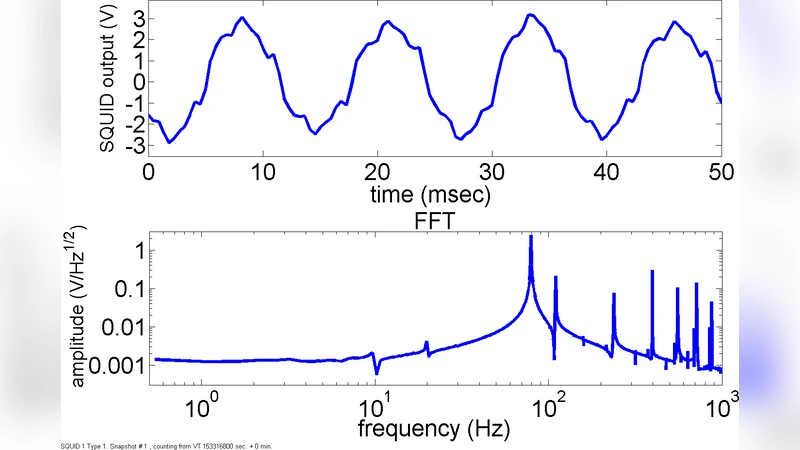
The paper presents a three‑stage algorithmic pipeline that extracts the instantaneous frequency and its time derivative from the high‑frequency (HF) SQUID signal recorded by the Gravity Probe B (GP‑B) mission with unprecedented nanohertz precision. GP‑B carried four ultra‑precise superconducting gyroscopes whose spin axes were monitored via SQUID magnetometers. Magnetic fluxons trapped on the gyroscope surface rotate with the body and induce a voltage modulation in the SQUID pickup loop at a frequency f z that is essentially the spin frequency f s plus a small contribution from the polhode motion (f p). The HF SQUID data are sampled at 2.2 kHz, segmented into 1.86‑second “snapshots” of 4096 points, and an on‑board FFT reduces each snapshot to 19 spectral bins (the central bin and its immediate neighbours for the first five harmonics and a 110 Hz calibration tone). The challenge is to recover f z with a resolution far finer than the 0.54 Hz FFT bin width.

Stage 1 – Frequency Interpolation.
Using the complex FFT values of the central bin (Fₙ) and its two neighbours (Fₙ₋₁, Fₙ₊₁), the authors form ratios Rₙ₊₁ = Fₙ₊₁/Fₙ and Rₙ₋₁ = Fₙ₋₁/Fₙ. By expanding the exact discrete Fourier transform expression around the unknown frequency offset xₙ = 2π(NΔt)(nf_d − f_z)/2 and retaining terms up to O(xₙ/N), they derive closed‑form interpolation formulas (Eqs. 7‑12). These give an estimate of f z with an intrinsic error of order 10⁻³ Hz. Because the HF signal contains strong odd harmonics (3 f z, 5 f z), the interpolation is performed separately on the fundamental, third, and fifth harmonics and the results are averaged, reducing systematic bias from spectral leakage and windowing effects.

Stage 2 – Phase Differencing.
The interpolated frequency provides a coarse estimate of the phase evolution. By computing the phase φ(t) of each snapshot at the estimated frequency and forming Δφ/Δt between successive snapshots, the authors obtain a direct measurement of the instantaneous frequency drift. This time‑domain technique exploits the full 1.86 s resolution of the raw data, achieving a drift resolution of ≈0.1 pHz s⁻¹, far superior to what could be inferred from the FFT alone.

Stage 3 – Model‑Based Bayesian Refinement.
The final algorithm integrates the physical model of gyroscope dynamics with the measurements from stages 1 and 2. The gyroscope’s angular momentum L and principal moments of inertia (I₁, I₂, I₃) determine the spin angle φ_s(t) via elliptic‑function expressions (Eqs. 2‑3). The observable HF frequency is f z = φ̇_s/(2π) + f_p, where f_p is the polhode frequency (≈0.1 mHz). Treating the interpolated frequencies and phase‑difference drifts as noisy observations, a Bayesian likelihood is constructed and explored with Markov‑Chain Monte Carlo sampling. This yields posterior distributions for φ̇_s and f_p with uncertainties of 30 nHz (≈5 × 10⁻¹⁰ relative accuracy) and 0.1 pHz s⁻¹, respectively. The method also accounts for the harmonic content of the signal and for any residual window‑function distortions.

Results and Impact.
Applying the full pipeline to six‑hour data segments from gyroscope 1, the authors demonstrate a stable frequency estimate with a spread of only 100 µHz after interpolation, which collapses to a 30 nHz scatter after the Bayesian refinement. The derived spin‑frequency drift matches the expected secular decay due to trapped flux relaxation, enabling a read‑out scale‑factor determination to 1 part in 10⁴. This precision translates into a gyroscope spin‑axis orientation accuracy of ~3 mas per orbit and a relativistic drift measurement (geodetic and frame‑dragging) accurate to ~20 mas yr⁻¹, meeting the primary science goals of GP‑B.

Broader Significance.
The work shows that, even with severely bandwidth‑limited telemetry, nanohertz‑level frequency metrology is achievable by (i) exploiting the analytic structure of the discrete Fourier transform, (ii) augmenting spectral information with phase‑difference time series, and (iii) embedding a realistic physical model within a Bayesian inference framework. The techniques are directly applicable to any precision rotation experiment, to space‑borne resonant sensors, and to laboratory systems where high‑Q oscillators must be tracked with sub‑µHz resolution.