Imaging Time-Series to Improve Classification and Imputation

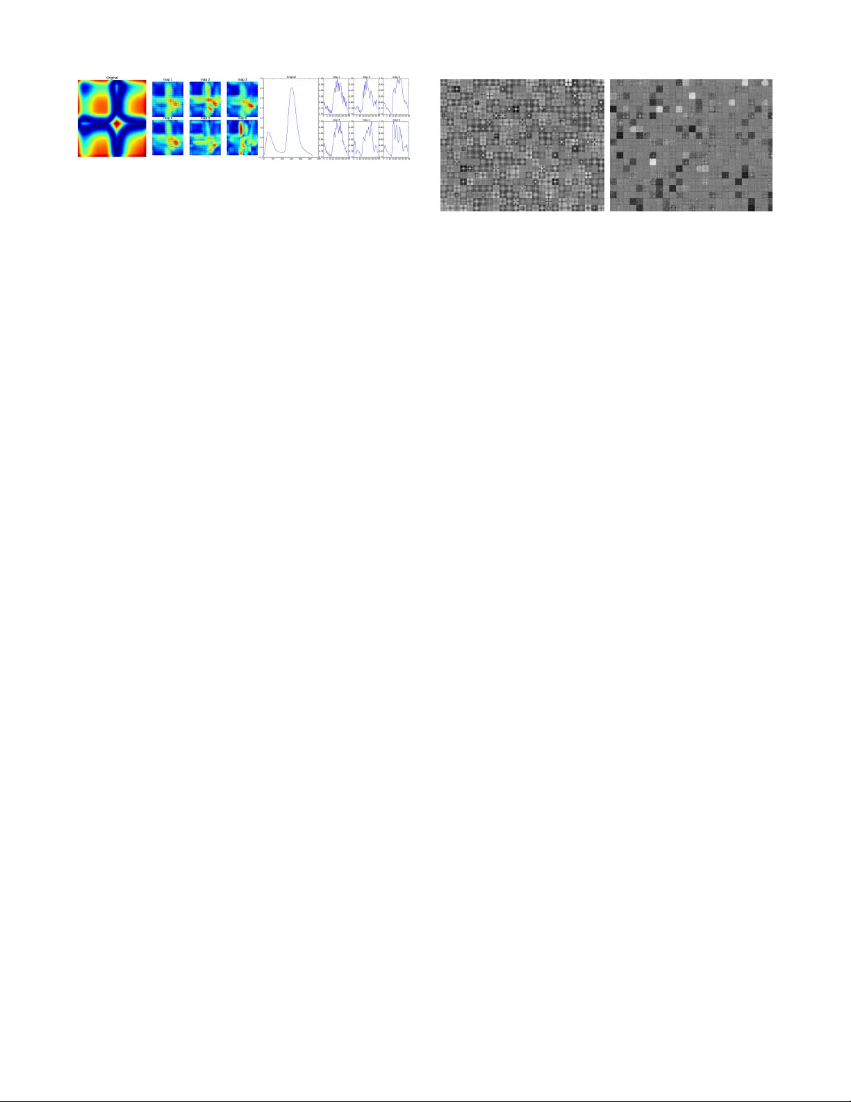
Imaging T ime-Series to Impr ov e Classification and Imputation Zhiguang W ang and Tim Oates Department of Computer Science and Electric Engineering Uni versity of Maryland, Baltimore County { stephen.wang, oates } @umbc.edu Abstract Inspired by recent successes of deep learning in computer vision, we propose a nov el frame- work for encoding time series as different types of images, namely , Gramian Angular Summa- tion/Difference Fields (GASF/GADF) and Markov T ransition Fields (MTF). This enables the use of techniques from computer vision for time series classification and imputation. W e used Tiled Con- volutional Neural Networks (tiled CNNs) on 20 standard datasets to learn high-lev el features from the individual and compound GASF-GADF-MTF images. Our approaches achie ve highly competi- tiv e results when compared to nine of the current best time series classification approaches. Inspired by the bijection property of GASF on 0/1 rescaled data, we train Denoised Auto-encoders (D A) on the GASF images of four standard and one synthesized compound dataset. The imputation MSE on test data is reduced by 12.18%-48.02% when compared to using the raw data. An analysis of the features and weights learned via tiled CNNs and D As ex- plains why the approaches work. 1 Introduction Since 2006, the techniques de veloped from deep neural net- works (or, deep learning) hav e greatly impacted natural lan- guage processing, speech recognition and computer vision research [ Bengio, 2009; Deng and Y u, 2014 ] . One suc- cessful deep learning architecture used in computer vision is con v olutional neural networks (CNN) [ LeCun et al. , 1998 ] . CNNs exploit translational inv ariance by extracting features through receptive fields [ Hubel and W iesel, 1962 ] and learn- ing with weight sharing, becoming the state-of-the-art ap- proach in various image recognition and computer vision tasks [ Krizhevsk y et al. , 2012 ] . Since unsupervised pretrain- ing has been shown to improve performance [ Erhan et al. , 2010 ] , sparse coding and T opographic Independent Compo- nent Analysis (TICA) are integrated as unsupervised pretrain- ing approaches to learn more div erse features with complex in v ariances [ Kavukcuoglu et al. , 2010; Ngiam et al. , 2010 ] . Along with the success of unsupervised pretraining applied in deep learning, others are studying unsupervised learning algorithms for generativ e models, such as Deep Belief Net- works (DBN) and Denoised Auto-encoders (D A) [ Hinton et al. , 2006; V incent et al. , 2008 ] . Many deep generati v e models are de veloped based on energy-based model or auto- encoders. T emporal autoencoding is integrated with Restrict Boltzmann Machines (RBMs) to improve generativ e mod- els [ H ¨ ausler et al. , 2013 ] . A training strategy inspired by recent work on optimization-based learning is proposed to train complex neural networks for imputation tasks [ Brakel et al. , 2013 ] . A generalized Denoised Auto-encoder ex- tends the theoretical framew ork and is applied to Deep Gen- erativ e Stochastic Networks (DGSN) [ Bengio et al. , 2013; Bengio and Thibodeau-Laufer , 2013 ] . Inspired by recent successes of supervised and unsuper- vised learning techniques in computer vision, we consider the problem of encoding time series as images to allow machines to “visually” recognize, classify and learn structures and pat- terns. Reformulating features of time series as visual clues has raised much attention in computer science and physics. In speech recognition systems, acoustic/speech data input is typ- ically represented by concatenating Mel-frequency cepstral coefficients (MFCCs) or perceptual linear predictiv e coeffi- cient (PLPs) [ Hermansky , 1990 ] . Recently , researchers are trying to build different network structures from time series for visual inspection or designing distance measures. Re- currence Networks were proposed to analyze the structural properties of time series from complex systems [ Donner et al. , 2010; 2011 ] . They build adjacency matrices from the predefined recurrence functions to interpret the time series as complex networks. Silva et al. extended the recurrence plot paradigm for time series classification using compression dis- tance [ Silva et al. , 2013 ] . Another way to build a weighted adjacency matrix is extracting transition dynamics from the first order Markov matrix [ Campanharo et al. , 2011 ] . Al- though these maps demonstrate distinct topological proper- ties among dif ferent time series, it remains unclear how these topological properties relate to the original time series since they ha ve no e xact in verse operations. W e present three nov el representations for encoding time series as images that we call the Gramian Angular Summa- tion/Difference Field (GASF/GADF) and the Markov T ransi- tion Field (MTF). W e applied deep T iled Con volutional Neu- ral Networks (T iled CNN) [ Ngiam et al. , 2010 ] to classify time series images on 20 standard datasets. Our e xperimental T im e Seri es x GA SF Polar Coordina te GADF Figure 1: Illustration of the proposed encoding map of Gramian Angular Fields. X is a sequence of rescaled time se- ries in the ’Fish’ dataset. W e transform X into a polar coordi- nate system by eq. (3) and finally calculate its GASF/GADF images with eqs. (5) and (7). In this example, we build GAFs without P AA smoothing, so the GAFs both hav e high resolu- tion. results demonstrate our approaches achieve the best perfor- mance on 9 of 20 standard dataset compared with 9 previous and current best classification methods. Inspired by the bi- jection property of GASF on 0 / 1 rescaled data, we train the Denoised Auto-encoder (D A) on the GASF images of 4 stan- dard and a synthesized compound dataset. The imputation MSE on test data is reduced by 12.18%-48.02% compared to using the raw data. An analysis of the features and weights learned via tiled CNNs and DA explains why the approaches work. 2 Imaging Time Series W e first introduce our two frameworks for encoding time se- ries as images. The first type of image is a Gramian Angular Field (GAF), in which we represent time series in a polar co- ordinate system instead of the typical Cartesian coordinates. In the Gramian matrix, each element is actually the cosine of the summation of angles. Inspired by previous work on the duality between time series and complex networks [ Campan- haro et al. , 2011 ] , the main idea of the second framework, the Marko v T ransition Field (MTF), is to build the Markov matrix of quantile bins after discretization and encode the dy- namic transition probability in a quasi-Gramian matrix. 2.1 Gramian Angular Field Giv en a time series X = { x 1 , x 2 , ..., x n } of n real-valued ob- servations, we rescale X so that all values fall in the interval [ − 1 , 1] or [0 , 1] by: ˜ x i − 1 = ( x i − max ( X )+( x i − min ( X )) max ( X ) − min ( X ) (1) or ˜ x i 0 = x i − min ( X ) max ( X ) − min ( X ) (2) Thus we can represent the rescaled time series ˜ X in polar coordinates by encoding the value as the angular cosine and the time stamp as the radius with the equation below:  φ = arccos ( ˜ x i ) , − 1 ≤ ˜ x i ≤ 1 , ˜ x i ∈ ˜ X r = t i N , t i ∈ N (3) In the equation above, t i is the time stamp and N is a con- stant factor to regularize the span of the polar coordinate sys- tem. This polar coordinate based representation is a novel way to understand time series. As time increases, correspond- ing values warp among different angular points on the span- ning circles, like water rippling. The encoding map of equa- tion 3 has two important properties. First, it is bijecti ve as cos( φ ) is monotonic when φ ∈ [0 , π ] . Giv en a time series, the proposed map produces one and only one result in the po- lar coordinate system with a unique in verse map. Second, as opposed to Cartesian coordinates, polar coordinates preserve absolute temporal relations. W e will discuss this in more de- tail in future work. Rescaled data in different intervals have different angular bounds. [0 , 1] corresponds to the cosine function in [0 , π 2 ] , while cosine values in the interval [ − 1 , 1] fall into the angu- lar bounds [0 , π ] . As we will discuss later, they provide dif- ferent information granularity in the Gramian Angular Field for classification tasks, and the Gramian Angular Difference Field (GADF) of [0 , 1] rescaled data has the accurate inv erse map. This property actually lays the foundation for imputing missing value of time series by reco v ering the images. After transforming the rescaled time series into the polar coordinate system, we can easily exploit the angular perspec- tiv e by considering the trigonometric sum/dif ference between each point to identify the temporal correlation within differ - ent time intervals. The Gramian Summation Angular Field (GASF) and Gramian Difference Angular Field (GADF) are defined as follows: GAS F = [ cos( φ i + φ j ) ] (4) = ˜ X 0 · ˜ X − p I − ˜ X 2 0 · p I − ˜ X 2 (5) GAD F = [ sin( φ i − φ j ) ] (6) = p I − ˜ X 2 0 · ˜ X − ˜ X 0 · p I − ˜ X 2 (7) I is the unit row vector [1 , 1 , ..., 1] . After transforming to the polar coordinate system, we take time series at each time step as a 1-D metric space. By defining the inner product < x, y > = x · y − √ 1 − x 2 · p 1 − y 2 and < x, y > = √ 1 − x 2 · y − x · p 1 − y 2 , two types of Gramian Angular Fields (GAFs) are actually quasi-Gramian matrices [ < ˜ x 1 , ˜ x 1 > ] . 1 The GAFs hav e sev eral advantages. First, they provide a way to preserv e temporal dependenc y , since time increases as the position moves from top-left to bottom-right. The GAFs contain temporal correlations because G ( i,j || i − j | = k ) repre- sents the relative correlation by superposition/difference of directions with respect to time interval k . The main diago- nal G i,i is the special case when k = 0 , which contains the original value/angular information. From the main diagonal, we can reconstruct the time series from the high le vel features learned by the deep neural network. Howe v er , the GAFs are large because the size of the Gramian matrix is n × n when the length of the raw time series is n . T o reduce the size of 1 ’quasi’ because the functions < x, y > we defined do not sat- isfy the property of linearity in inner-product space. 0 . 944 0 . 0 5 6 0 . 0 5 6 0 . 860 0 0 0 . 084 0 0 0 . 085 0 0 0 . 840 0 . 075 0 . 075 0 . 925 A B C D A B C D T im e Series x Markov T ransit ion Matri x MTF Figure 2: Illustration of the proposed encoding map of Markov Transition Fields. X is a sequence of time-series in the ’ECG’ dataset . X is first discretized into Q quantile bins. Then we calculate its Markov Transition Matrix W and fi- nally build its MTF with eq. (8). the GAFs, we apply Piecewise Aggregation Approximation (P AA) [ Keogh and Pazzani, 2000 ] to smooth the time series while preserving the trends. The full pipeline for generating the GAFs is illustrated in Figure 1. 2.2 Marko v T ransition Field W e propose a framework similar to Campanharo et al. for encoding dynamical transition statistics, b ut we extend that idea by representing the Marko v transition probabilities se- quentially to preserve information in the time domain. Giv en a time series X , we identify its Q quantile bins and assign each x i to the corresponding bins q j ( j ∈ [1 , Q ] ). Thus we construct a Q × Q weighted adjacency matrix W by count- ing transitions among quantile bins in the manner of a first- order Marko v chain along the time axis. w i,j is gi ven by the frequency with which a point in quantile q j is followed by a point in quantile q i . After normalization by P j w ij = 1 , W is the Markov transition matrix. It is insensitiv e to the distri- bution of X and temporal dependenc y on time steps t i . How- ev er , our experimental results on W demonstrate that getting rid of the temporal dependency results in too much informa- tion loss in matrix W . T o ov ercome this drawback, we define the Markov T ransition Field (MTF) as follows: M =     w ij | x 1 ∈ q i ,x 1 ∈ q j · · · w ij | x 1 ∈ q i ,x n ∈ q j w ij | x 2 ∈ q i ,x 1 ∈ q j · · · w ij | x 2 ∈ q i ,x n ∈ q j . . . . . . . . . w ij | x n ∈ q i ,x 1 ∈ q j · · · w ij | x n ∈ q i ,x n ∈ q j     (8) W e b uild a Q × Q Markov transition matrix ( W ) by di vid- ing the data (magnitude) into Q quantile bins. The quantile bins that contain the data at time stamp i and j (temporal axis) are q i and q j ( q ∈ [1 , Q ] ). M ij in the MTF denotes the tran- sition probability of q i → q j . That is, we spread out matrix W which contains the transition probability on the magnitude axis into the MTF matrix by considering the temporal posi- tions. By assigning the probability from the quantile at time step i to the quantile at time step j at each pixel M ij , the MTF M actually encodes the multi-span transition probabilities of ... ... F ea tur e map s 𝑙 = 6 Con volutional I TIC A Pool ing I ... ... Con volutional I I TIC A Pool ing I I ... Linear SV M Rec ept ive Fiel d 8 × 8 Rec ept ive Fiel d 3 × 3 U nti ed w eig hts k = 2 P oo l ing Size 3 × 3 P oo l ing Size 3 × 3 Figure 3: Structure of the tiled con v olutional neural networks. W e fix the size of recepti ve fields to 8 × 8 in the first con volu- tional layer and 3 × 3 in the second conv olutional layer . Each TICA pooling layer pools over a block of 3 × 3 input units in the previous layer without warping around the borders to optimize for sparsity of the pooling units. The number of pooling units in each map is exactly the same as the number of input units. The last layer is a linear SVM for classifica- tion. W e construct this network by stacking two T iled CNNs, each with 6 maps ( l = 6 ) and tiling size k = 1 , 2 , 3 . the time series. M i,j || i − j | = k denotes the transition probabil- ity between the points with time interval k . For example, M ij | j − i =1 illustrates the transition process along the time axis with a skip step. The main diagonal M ii , which is a special case when k = 0 captures the probability from each quantile to itself (the self-transition probability) at time step i . T o make the image size manageable and computation more efficient, we reduce the MTF size by averaging the pixels in each non-overlapping m × m patch with the blurring kernel { 1 m 2 } m × m . That is, we aggregate the transition probabilities in each subsequence of length m together . Figure 2 sho ws the procedure to encode time series to MTF . 3 Classify Time Series Using GAF/MTF with Tiled CNNs W e apply Tiled CNNs to classify time series using GAF and MTF representations on 20 datasets from [ Keogh et al. , 2011 ] in different domains such as medicine, entomology , engineer - ing, astronomy , signal processing, and others. The datasets are pre-split into training and testing sets to facilitate ex- perimental comparisons. W e compare the classification er- ror rate of our GASF-GADF-MTF approach with previously published results of 3 competing methods and 6 best ap- proaches proposed recently: early state-of-the-art 1NN clas- sifiers based on Euclidean distance and DTW (Best W arp- ing Windo w and no W arping W indo w), Fast-Shapelets [ Rak- thanmanon and Keogh, 2013 ] , a 1NN classifier based on SAX with Bag-of-Patterns (SAX-BoP) [ Lin et al. , 2012 ] , a SAX based V ector Space Model (SAX-VSM) [ Senin and Ma- linchik, 2013 ] , a classifier based on the Recurrence Patterns Compression Distance(RPCD) [ Silva et al. , 2013 ] , a tree- based symbolic representation for multiv ariate time series (SMTS) [ Baydogan and Runger , 2014 ] and a SVM classifier based on a bag-of-features representation (TSBF) [ Baydogan T able 1: Summary of error rates for 3 classic baselines, 6 recently published best results and our approach. The symbols  , ∗ , † and • represent datasets generated from human motions, figure shapes, synthetically predefined procedures and all remaining temporal signals, respectiv ely . For our approach, the numbers in brack ets are the optimal P AA size and quantile size. Dataset 1NN- 1NN-DTW - 1NN-DTW - Fast- SAX- SAX- RPCD SMTS TSBF GASF-GADF- RA W BWW nWW Shapelet BoP VSM MTF 50words • 0.369 0.242 0.31 N/A 0.466 N/A 0.2264 0.289 0.209 0.301 (16, 32) Adiac ∗ 0.389 0.391 0.396 0.514 0.432 0.381 0.3836 0.248 0.245 0.373 (32, 48) Beef • 0.467 0.467 0.5 0.447 0.433 0.33 0.3667 0.26 0.287 0.233 (64, 40) CBF † 0.148 0.004 0.003 0.053 0.013 0.02 N/A 0.02 0.009 0.009 (32, 24) Coffee • 0.25 0.179 0.179 0.068 0.036 0 0 0.029 0.004 0 (64, 48) ECG • 0.12 0.12 0.23 0.227 0.15 0.14 0.14 0.159 0.145 0.09 (8, 32) FaceAll ∗ 0.286 0.192 0.192 0.411 0.219 0.207 0.1905 0.191 0.234 0.237 (8, 48) FaceF our ∗ 0.216 0.114 0.17 0.090 0.023 0 0.0568 0.165 0.051 0.068 (8, 16) fish ∗ 0.217 0.16 0.167 0.197 0.074 0.017 0.1257 0.147 0.08 0.114 (8, 40) Gun Point / 0.087 0.087 0.093 0.061 0.027 0.007 0 0.011 0.011 0.08 (32, 32) Lighting2 • 0.246 0.131 0.131 0.295 0.164 0.196 0.2459 0.269 0.257 0.114 (16, 40) Lighting7 • 0.425 0.288 0.274 0.403 0.466 0.301 0.3562 0.255 0.262 0.260 (16, 48) Oliv eOil • 0.133 0.167 0.133 0.213 0.133 0.1 0.1667 0.177 0.09 0.2 (8, 48) OSULeaf ∗ 0.483 0.384 0.409 0.359 0.256 0.107 0.3554 0.377 0.329 0.358 (16, 32) SwedishLeaf ∗ 0.213 0.157 0.21 0.269 0.198 0.01 0.0976 0.08 0.075 0.065 (16, 48) synthetic control † 0.12 0.017 0.007 0.081 0.037 0.251 N/A 0.025 0.008 0.007 (64, 48) T race † 0.24 0.01 0 0.002 0 0 N/A 0 0.02 0 (64, 48) T wo Patterns † 0.09 0.0015 0 0.113 0.129 0.004 N/A 0.003 0.001 0.091 (64, 32) wafer • 0.005 0.005 0.02 0.004 0.003 0.0006 0.0034 0 0.004 0 (64, 16) yoga ∗ 0.17 0.155 0.164 0.249 0.17 0.164 0.134 0.094 0.149 0.196 (8, 32) #wins 0 0 3 0 1 5 3 4 4 9 et al. , 2013 ] . 3.1 Tiled Con volutional Neural Networks T iled Con v olutional Neural Networks are a v ariation of Con- volutional Neural Networks that use tiles and multiple fea- ture maps to learn in v ariant features. T iles are parame- terized by a tile size k to control the distance over which weights are shared. By producing multiple feature maps, T iled CNNs learn overcomplete representations through un- supervised pretraining with T opographic ICA (TICA). For the sake of space, please refer to [ Ngiam et al. , 2010 ] for more details. The structure of T iled CNNs applied in this paper is illustrated in Figure 3. 3.2 Experiment Setting In our experiments, the size of the GAF image is regulated by the the number of P AA bins S GAF . Gi ven a time se- ries X of size n , we divide the time series into S GAF ad- jacent, non-overlapping windo ws along the time axis and ex- tract the means of each bin. This enables us to construct the smaller GAF matrix G S GAF × S GAF . MTF requires the time series to be discretized into Q quantile bins to calculate the Q × Q Marko v transition matrix, from which we construct the raw MTF image M n × n afterwards. Before classifica- tion, we shrink the MTF image size to S M T F × S M T F by the blurring kernel { 1 m 2 } m × m where m = d n S M T F e . The T iled CNN is trained with image size { S GAF , S M T F } ∈ { 16 , 24 , 32 , 40 , 48 } and quantile size Q ∈ { 8 , 16 , 32 , 64 } . At the last layer of the T iled CNN, we use a linear soft margin SVM [ Fan et al. , 2008 ] and select C by 5-fold cross v alida- tion ov er { 10 − 4 , 10 − 3 , . . . , 10 4 } on the training set. For each input of image size S GAF or S M T F and quan- tile size Q , we pretrain the T iled CNN with the full unlabeled dataset (both training and test set) to learn the initial weights W through TICA. Then we train the SVM at the last layer by selecting the penalty factor C with cross validation. Fi- nally , we classify the test set using the optimal hyperparame- ters { S, Q, C } with the lowest error rate on the training set. If two or more models tie, we prefer the larger S and Q because larger S helps preserve more information through the P AA procedure and lar ger Q encodes the dynamic transition statis- tics with more detail. Our model selection approach provides generalization without being overly expensi ve computation- ally . 3.3 Results and Discussion W e use T iled CNNs to classify the single GASF , GADF and MTF images as well as the compound GASF-GADF-MTF images on 20 datasets. For the sak e of space, we do not sho w the full results on single-channel images. Generally , our ap- proach is not prone to overfitting by the relativ ely small dif- ference between training and test set errors. One exception is the Oliv e Oil dataset with the MTF approach where the test error is significantly higher . In addition to the risk of potential overfitting, we found that MTF has generally higher error rates than GAFs. This is most likely because of the uncertainty in the in v erse map of MTF . Note that the encoding function from − 1 / 1 rescaled time series to GAFs and MTF are both surjections. The map functions of GAFs and MTF will each produce only one im- age with fixed S and Q for each giv en time series X . Be- cause they are both surjecti ve mapping functions, the in v erse image of both mapping functions is not fixed. Howe ver , the Figure 4: Pipeline of time series imputation by image re- cov ery . Raw GASF → ”broken” GASF → recovered GASF (top), Raw time series → corrupted time series with missing value → predicted time series (bottom) on dataset ”Swedish- Leaf” (left) and ”ECG” (right). mapping function of GAFs on 0 / 1 rescaled time series are bijectiv e. As shown in a later section, we can reconstruct the raw time series from the diagonal of GASF , but it is very hard to even roughly recover the signal from MTF . Even for − 1 / 1 rescaled data, the GAFs hav e smaller uncertainty in the inv erse image of their mapping function because such randomness only comes from the ambiguity of cos( φ ) when φ ∈ [0 , 2 π ] . MTF , on the other hand, has a much larger in- verse image space, which results in large v ariations when we try to recover the signal. Although MTF encodes the transi- tion dynamics which are important features of time series, such features alone seem not to be sufficient for recogni- tion/classification tasks. Note that at each pixel, G ij denotes the supersti- tion/difference of the directions at t i and t j , M ij is the tran- sition probability from the quantile at t i to the quantile at t j . GAF encodes static information while MTF depicts informa- tion about dynamics. From this point of view , we consider them as three “orthogonal” channels, like different colors in the RGB image space. Thus, we can combine GAFs and MTF images of the same size (i.e. S GAF s = S M T F ) to construct a triple-channel image (GASF-GADF-MTF). It combines both the static and dynamic statistics embedded in the raw time series, and we posit that it will be able to enhance classifica- tion performance. In the experiments below , we pretrain and tune the Tiled CNN on the compound GASF-GADF-MTF images. Then, we report the classification error rate on test sets. In T able 1, the T iled CNN classifiers on GASF-GADF- MTF images achiev ed significantly competitive results with 9 other state-of-the-art time series classification approaches. 4 Image Recovery on GASF f or Time Series Imputation with Denoised A uto-encoder As pre viously mentioned, the mapping functions from − 1 / 1 rescaled time series to GAFs are surjections. The uncertainty among the inv erse images come from the ambiguity of the cos( φ ) when φ ∈ [0 , 2 π ] . Howe v er the mapping functions of 0 / 1 rescaled time series are bijections. The main diagonal of GASF , i.e. { G ii } = { cos(2 φ i ) } allo ws us to precisely reconstruct the original time series by cos( φ ) = r cos(2 φ ) + 1 2 φ ∈ [0 , π 2 ] (9) Thus, we can predict missing values among time series through recovering the ”broken” GASF images. During train- ing, we manually add ”salt-and-pepper” noise (i.e., randomly set a number of points to 0) to the raw time series and trans- form the data to GASF images. Then a single layer Denoised Auto-encoder (D A) is fully trained as a generati ve model to reconstruct GASF images. Note that at the input layer , we do not add noise again to the ”broken” GASF images. A Sigmoid function helps to learn the nonlinear features at the hidden layer . At the last layer we compute the Mean Square Error (MSE) between the original and ”broken” GASF im- ages as the loss function to ev aluate fitting performance. T o train the models simple batch gradient descent is applied to back propagate the inference loss. For testing, after we cor- rupt the time series and transform the noisy data to ”broken” GASF , the trained D A helps recov er the image, on which we extract the main diagonal to reconstruct the recovered time series. T o compare the imputation performance, we also test standard D A with the ra w time series data as input to recover the missing values (Figure. 4). 4.1 Experiment Setting For the DA models we use batch gradient descent with a batch size of 20. Optimization iterations run until the MSE changed less than a threshold of 10 − 3 for GASF and 10 − 5 for raw time series. A single hidden layer has 500 hidden neurons with sigmoid functions. W e choose four dataset of dif ferent types from the UCR time series repository for the imputation task: ”Gun Point” (human motion), ”CBF” (synthetic data), ”SwedishLeaf” (figure shapes) and ”ECG” (other remaining temporal signals). T o explore if the statistical dependency learned by the DA can be generalized to unknown data, we use the abov e four datasets and the ”Adiac” dataset together to train the D A to impute two totally unknown test datasets, ”T wo Patterns” and ”wafer” (W e name these synthetic miscel- laneous datasets ”7 Misc”). T o add randomness to the input of D A, we randomly set 20% of the raw data among a specific time series to be zero (salt-and-pepper noise). Our experi- ments for imputation are implemented with Theano [ Bastien et al. , 2012 ] . T o control for the random initialization of the parameters and the randomness induced by gradient descent, we repeated every experiment 10 times and report the av erage MSE. 4.2 Results and Discussion T able 2: MSE of imputation on time series using ra w data and GASF images. Dataset Full MSE Interpolation MSE Raw GASF Raw GASF ECG 0.01001 0.01148 0.02301 0.01196 CBF 0.02009 0.03520 0.04116 0.03119 Gun Point 0.00693 0.00894 0.01069 0.00841 SwedishLeaf 0.00606 0.00889 0.01117 0.00981 7 Misc 0.06134 0.10130 0.10998 0.07077 In T able 2, ”Full MSE” means the MSE between the com- plete recovered and original sequence and ”Imputation MSE” Figure 5: (a) Original GASF and its six learned feature maps before the SVM layer in Tiled CNNs (left). (b) Raw time series and its reconstructions from the main diagonal of six feature maps on ’50W ords’ dataset (right). means the MSE of only the unknown points among each time series. Interestingly , DA on the raw data perform well on the whole sequence, generally , b ut there is a gap between the full MSE and imputation MSE. That is, D A on raw time series can fit the known data much better than predicting the un- known data (like overfitting). Predicting the missing value using GASF always achiev es slightly higher full MSE b ut the imputation MSE is reduced by 12.18%-48.02%. W e can ob- serve that the difference between the full MSE and imputation MSE is much smaller on GASF than on the raw data. Inter- polation with GASF has more stable performance than on the raw data. Why does predicting missing v alues using GASF have more stable performance than using raw time series? Actu- ally , the transformation maps of GAFs are generally equiv a- lent to a kernel trick. By defining the inner product k ( x i , x j ) , we achiev e data augmentation by increasing the dimension- ality of the raw data. By preserving the temporal and spatial information in GASF images, the D A utilizes both temporal and spatial dependencies by considering the missing points as well as their relations to other data that has been explicitly en- coded in the GASF images. Because the entire sequence, in- stead of a short subsequence, helps predict the missing value, the performance is more stable as the full MSE and imputa- tion MSE are close. 5 Analysis on F eatur es and W eights Learned by Tiled CNNs and D A In contrast to the cases in which the CNNs is applied in nat- ural image recognition tasks, neither GAFs nor MTF hav e natural interpretations of visual concepts like “edges” or “an- gles”. In this section we analyze the features and weights learned through Tiled CNNs to explain why our approach works. Figure 5 illustrates the reconstruction results from six fea- ture maps learned through the T iled CNNs on GASF (by Eqn 9). The T iled CNNs extracts the color patch, which is essen- tially a moving av erage that enhances se veral recepti v e fields within the nonlinear units by different trained weights. It is not a simple moving av erage but the synthetic integration by considering the 2D temporal dependencies among different time interv als, which is a benefit from the Gramian matrix structure that helps preserve the temporal information. By ob- serving the orthogonal reconstruction from each layer of the feature maps, we can clearly observe that the tiled CNNs can extract the multi-frequency dependencies through the con v o- Figure 6: All 500 filters learned by D A on the ”Gun Point” (left) and ”7 Misc” (right) dataset. lution and pooling architecture on the GAF and MTF images to preserve the trend while addressing more details in differ - ent subphases. The high-leveled feature maps learned by the T iled CNN are equiv alent to a multi-frequency approxima- tor of the original curve. Our experiments also demonstrates the learned weight matrix W with the constraint W W T = I , which makes ef fecti ve use of local orthogonality . The TICA pretraining provides the built-in advantage that the function w .r .t the parameter space is not likely to be ill-conditioned as W W T = 1 . The weight matrix W is quasi-orthogonal and approaching 0 without large magnitude. This implies that the condition number of W approaches 1 and helps the system to be well-conditioned. As for imputation, because the GASF images have no con- cept of ”angle” and ”edge”, D A actually learned different pro- totypes of the GASF images (T able 6). W e find that there is significant noise in the filters on the ”7 Misc” dataset because the training set is relativ ely small to better learn different fil- ters. Actually , all the noisy filters with no patterns work like one Gaussian noise filter . 6 Conclusions and Future W ork W e created a pipeline for conv erting time series into novel representations, GASF , GADF and MTF images, and ex- tracted multi-level features from these using Tiled CNN and D A for classification and imputation. W e demonstrated that our approach yields competitiv e results for classifica- tion when compared to recently best methods. Imputation using GASF achieved better and more stable performance than on the raw data using DA. Our analysis of the features learned from T iled CNN suggested that Tiled CNN works like a multi-frequency moving av erage that benefits from the 2D temporal dependency that is preserved by Gramian matrix. Features learned by D A on GASF is shown to be dif ferent prototype, as correlated basis to construct the raw images. Important future work will inv olv e dev eloping recurrent neural nets to process streaming data. W e are also quite inter - ested in ho w dif ferent deep learning architectures perform on the GAFs and MTF images. Another important future work is to learn deep generative models with more high-lev el fea- tures on GAFs images. W e aim to further apply our time se- ries models in real world regression/imputation and anomaly detection tasks. References [ Bastien et al. , 2012 ] Fr ´ ed ´ eric Bastien, P ascal Lamblin, Razv an Pascanu, James Bergstra, Ian J. Goodfellow , Arnaud Bergeron, Nicolas Bouchard, and Y oshua Bengio. Theano: new features and speed impro vements. Deep Learning and Unsupervised Fea- ture Learning NIPS 2012 W orkshop, 2012. [ Baydogan and Runger , 2014 ] Mustafa Gokce Baydogan and George Runger . Learning a symbolic representation for multi- variate time series classification. Data Mining and Knowledge Discovery , pages 1–23, 2014. [ Baydogan et al. , 2013 ] Mustafa Gokce Baydogan, Geor ge Runger, and Eugene T uv . A bag-of-features framework to classify time series. P attern Analysis and Machine Intelligence, IEEE T r ans- actions on , 35(11):2796–2802, 2013. [ Bengio and Thibodeau-Laufer , 2013 ] Y oshua Bengio and Eric Thibodeau-Laufer . Deep generativ e stochastic networks trainable by backprop. arXiv preprint , 2013. [ Bengio et al. , 2013 ] Y oshua Bengio, Li Y ao, Guillaume Alain, and Pascal V incent. Generalized denoising auto-encoders as genera- tiv e models. In Advances in Neural Information Pr ocessing Sys- tems , pages 899–907, 2013. [ Bengio, 2009 ] Y oshua Bengio. Learning deep architectures for ai. F oundations and trends R  in Machine Learning , 2(1):1–127, 2009. [ Brakel et al. , 2013 ] Phil ´ emon Brakel, Dirk Stroobandt, and Ben- jamin Schrauwen. T raining energy-based models for time- series imputation. The Journal of Machine Learning Resear c h , 14(1):2771–2797, 2013. [ Campanharo et al. , 2011 ] Andriana SLO Campanharo, M Irmak Sirer , R Dean Malmgren, Fernando M Ramos, and Lu ´ ıs A Nunes Amaral. Duality between time series and networks. PloS one , 6(8):e23378, 2011. [ Deng and Y u, 2014 ] Li Deng and Dong Y u. Deep learning: Meth- ods and applications. T echnical Report MSR-TR-2014-21, Jan- uary 2014. [ Donner et al. , 2010 ] Reik V Donner , Y ong Zou, Jonathan F Donges, Norbert Marwan, and J ¨ urgen Kurths. Recurrence net- worksa nov el paradigm for nonlinear time series analysis. New Journal of Physics , 12(3):033025, 2010. [ Donner et al. , 2011 ] Reik V Donner , Michael Small, Jonathan F Donges, Norbert Marwan, Y ong Zou, Ruoxi Xiang, and J ¨ urgen Kurths. Recurrence-based time series analysis by means of com- plex network methods. International Journal of Bifurcation and Chaos , 21(04):1019–1046, 2011. [ Erhan et al. , 2010 ] Dumitru Erhan, Y oshua Bengio, Aaron Courville, Pierre-Antoine Manzagol, Pascal V incent, and Samy Bengio. Why does unsupervised pre-training help deep learning? The Journal of Machine Learning Resear ch , 11:625–660, 2010. [ Fan et al. , 2008 ] Rong-En Fan, Kai-W ei Chang, Cho-Jui Hsieh, Xiang-Rui W ang, and Chih-Jen Lin. Liblinear: A library for large linear classification. The Journal of Machine Learning Researc h , 9:1871–1874, 2008. [ H ¨ ausler et al. , 2013 ] Chris H ¨ ausler , Alex Susemihl, Martin P Nawrot, and Manfred Opper . T emporal autoencoding im- prov es generati ve models of time series. arXiv pr eprint arXiv:1309.3103 , 2013. [ Hermansky , 1990 ] Hynek Hermansky . Perceptual linear predictive (plp) analysis of speech. the Journal of the Acoustical Society of America , 87(4):1738–1752, 1990. [ Hinton et al. , 2006 ] Geoffre y Hinton, Simon Osindero, and Y ee- Whye T eh. A f ast learning algorithm for deep belief nets. Neural computation , 18(7):1527–1554, 2006. [ Hubel and W iesel, 1962 ] David H Hubel and T orsten N Wiesel. Receptiv e fields, binocular interaction and functional architecture in the cat’ s visual cortex. The Journal of physiology , 160(1):106, 1962. [ Kavukcuoglu et al. , 2010 ] K oray Kavukcuoglu, Pierre Sermanet, Y -Lan Boureau, Karol Gregor , Micha ¨ el Mathieu, and Y ann L Cun. Learning con v olutional feature hierarchies for visual recog- nition. In Advances in neural information pr ocessing systems , pages 1090–1098, 2010. [ Keogh and P azzani, 2000 ] Eamonn J Keogh and Michael J Paz- zani. Scaling up dynamic time warping for datamining appli- cations. In Pr oceedings of the sixth ACM SIGKDD international confer ence on Knowledge discovery and data mining , pages 285– 289. A CM, 2000. [ Keogh et al. , 2011 ] Eamonn Keogh, Xiaopeng Xi, Li W ei, and Chotirat Ann Ratanamahatana. The ucr time series classifica- tion/clustering homepage. URL= http://www . cs. ucr . edu/˜ ea- monn/time series data , 2011. [ Krizhevsk y et al. , 2012 ] Alex Krizhe vsky , Ilya Sutskev er , and Ge- offre y E Hinton. Imagenet classification with deep con v olutional neural networks. In Advances in neural information processing systems , pages 1097–1105, 2012. [ LeCun et al. , 1998 ] Y ann LeCun, L ´ eon Bottou, Y oshua Bengio, and Patrick Haf fner . Gradient-based learning applied to docu- ment recognition. Proceedings of the IEEE , 86(11):2278–2324, 1998. [ Lin et al. , 2012 ] Jessica Lin, Rohan Khade, and Y uan Li. Rotation- in variant similarity in time series using bag-of-patterns represen- tation. Journal of Intelligent Information Systems , 39(2):287– 315, 2012. [ Ngiam et al. , 2010 ] Jiquan Ngiam, Zhenghao Chen, Daniel Chia, Pang W K oh, Quoc V Le, and Andre w Y Ng. Tiled conv olutional neural networks. In Advances in Neural Information Pr ocessing Systems , pages 1279–1287, 2010. [ Rakthanmanon and Keogh, 2013 ] Thanawin Rakthanmanon and Eamonn K eogh. Fast shapelets: A scalable algorithm for dis- cov ering time series shapelets. In Pr oceedings of the thirteenth SIAM confer ence on data mining (SDM) . SIAM, 2013. [ Senin and Malinchik, 2013 ] Pa vel Senin and Sergey Malinchik. Sax-vsm: Interpretable time series classification using sax and vector space model. In Data Mining (ICDM), 2013 IEEE 13th International Confer ence on , pages 1175–1180. IEEE, 2013. [ Silva et al. , 2013 ] Diego F Silva, V inicius Souza, MA De, and Gustav o EAP A Batista. Time series classification using compres- sion distance of recurrence plots. In Data Mining (ICDM), 2013 IEEE 13th International Conference on , pages 687–696. IEEE, 2013. [ V incent et al. , 2008 ] Pascal V incent, Hugo Larochelle, Y oshua Bengio, and Pierre-Antoine Manzagol. Extracting and compos- ing robust features with denoising autoencoders. In Pr oceedings of the 25th international conference on Machine learning , pages 1096–1103. A CM, 2008.