Scalable Multi-Output Label Prediction: From Classifier Chains to Classifier Trellises

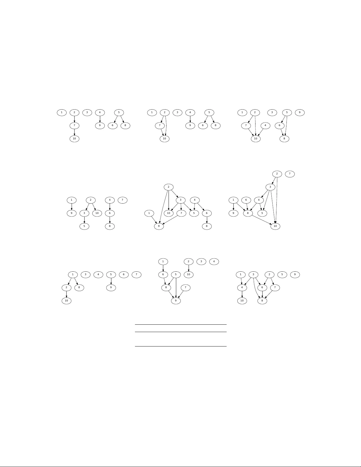
SCALABLE MUL TI-OUTPUT LABEL PREDICTION: FR OM CLASSIFIER CHAINS TO CLASSIFIER TRELLISES J . Read 1 , L. Martino 2 , P . M. Olmos 3 , David Luengo 4 1 Dep. of Computer Science, Aalto Uni versity and HIIT , Helsinki, Finland ( jesse.read@aalto.fi ). 2 Dep. of Mathematics and Statistics, Uni versity of Helsinki, Helsinki (Finland). 3 Dep. of Signal Theory and Communications, Uni versidad Carlos III de Madrid (Spain) . 4 Dep. of Circuits and Systems Engineering, Uni versidad Polit ´ ecnica de Madrid, (Spain). ABSTRA CT Multi-output inference tasks, such as multi-label classification, have become increasingly important in recent years. A popular method for multi-label classification is classifier chains , in which the predictions of individual classifiers are cascaded along a chain, thus taking into account inter-label dependencies and improving the ov erall performance. Sev eral v arieties of classifier chain methods hav e been introduced, and many of them perform v ery competiti vely across a wide range of benchmark datasets. Howe v er , scalability limitations become apparent on larger datasets when modeling a fully-cascaded chain. In particular, the methods’ strategies for discov ering and modeling a good chain structure constitutes a mayor computational bottleneck. In this paper , we present the classifier tr ellis (CT) method for scalable multi-label classification. W e compare CT with several recently proposed classifier chain methods to show that it occupies an important niche: it is highly competitive on standard multi-label problems, yet it can also scale up to thousands or ev en tens of thousands of labels. K e ywor ds: classifier chains; multi-label classification; multi-output prediction; structured inference; Bayesian netw orks 1. INTR ODUCTION Multi-output classification (MOC) (also kno wn variously as multi-target, multi-objecti ve, and multidimensional classification) is the supervised learning problem where an instance is associated with a set of qualitative discrete variables (a.k.a. labels ), rather than with a single v ariable 1 . Since these label variables are often strongly correlated, modeling the dependencies between them allows MOC methods to improv e their performance at the expense of an increased computational cost. Multi-label classification (MLC) is a special case of MOC where all the labels are binary; it has already attracted a great deal of interest and de velopment in machine learning literature ov er the last fe w years. In [27], the authors giv e a recent re view of, and many references to, a number of recent and popular methods for MLC. Figure 1 shows the relationship between dif ferent classification paradigms, according to the number of labels ( L = 1 vs. L > 1 ) and their type (binary [ K = 2] or not [ K > 2] ). There are a v ast range of acti ve applications of MLC, including tagging images, categorizing documents, and labelling video and other media, and learning the relationship among genes and biological functions. Labels (e.g., tags, categories, genres) are either relev ant or not. For example, an image may be labelled beach and urban ; a ne ws article may be sectioned under europe and economy . Relev ance is usually indicated by 1 , and irrelev ance by 0 . The general MOC scheme may add other information such as month, age, or gender . Note that month ∈ { 1 , . . . , 12 } and therefore is not simply irrelev ant or not. This MOC task has received relativ ely less attention than MLC (although there is some work emerging, e.g., [25] and [17]). Howe v er , most MLC-transformation methods (e.g., treating each label variable as a separate multi-class problem) are equally applicable to MOC. Indeed, in this paper we deal with a family of methods based on this approach. Note also that, as any integer can be represented in binary form (e.g., 3 ⇔ [0 , 0 , 0 , 1 , 1] ), any MOC task can ‘decode’ into a MLC task and vice versa. In this paper , we focus on scalable MLC methods, able to effecti vely deal with large datasets at feasible complexity . Many recent MLC methods, particularly those based on classifier chains, tend to be over engineered, in vesting evermore computational power to model label dependencies, but presenting poor scalability properties. In the first part of the paper, we revie w some 1 W e henceforth try to av oid the use of the term ‘class’; it generates confusion since it is used v ariously in the literature to refer to both the tar get variable, and a value that the v ariable takes. Rather , we refer to label v ariables, each of which takes a number of values . state-of-the-art methods from the MLC and MOC literature to sho w that the more powerful solutions are not well-suited to deal with large-size label sets. For instance, classifier chains [3, 20] consider a full cascade of labels along a chain to model their joint probability distribution and, either they explore all possible label orders in the chain, incurring in exponential complexity with the number of labels, or they compare a small subset of them chosen at random, which is inef fecti ve for large dimensional problems. The main contribution of the paper is a novel highly-scalable method: the classifier trellis (CT). Rather than imposing a long-range and ultimately computationally complex dependency model, as in classifier chains, CT captures the essential depen- dencies among labels very ef ficiently . This is achie v ed by considering a predefined trellis structure for the underlying graphical model, where dependent nodes (labels) are sequentially placed in the structure according to easily-computable probabilistic measures. Experimental results across a wide set of datasets show that CT is able to scale up to large sets (namely , thousands and tens of thousands of labels) while remaining very competitiv e on standard MLC problems. In fact, in most of our experi- ments, CT was very close to the running time of the nai ve baseline method, which ne glects any statistical dependency between labels. Also, an ensemble version of CT , where the method is run multiple times with dif ferent random seeds and classification is done through majority voting, does not significantly outperform the single-shot CT . This demonstrates that our method is quite robust against initialization. The paper is organized as follo ws. First, in Section 2 we formalize the notation and describe the problem’ s setting. In Section 3 we revie w some state-of-the-art methods from the MLC and MOC literature, as well as their various strategies for modeling label dependence. This revie w is augmented with empirical results. In Section 4 we make use of the studies and theory from earlier sections to present the classifier trellis (CT) method. In Section 5 we carry out two sets of experiments: firstly we compare CT to some state-of-the-art multi-label methods on an MLC task; and secondly , we show that CT can also provide competitive performance on typical structured output prediction task (namely localization via segmentation). Finally , in Section 6 we discuss the results and take conclusions. T wo appendixes ha ve been included to help the readability of the paper and support the presented results. In A, we compare two low-comple xity methods to infer the label dependencies from training data. In B we revie w Monte Carlo methods, which are required in this paper to perform probabilistic approximate inference of the label set associated to a new test input. 2. PR OBLEM SETUP AND NO T A TION Follo wing a standard machine learning notation, the n -th feature vector can be represented as x ( n ) = [ x ( n ) 1 , . . . , x ( n ) D ] > ∈ X = X 1 × · · · × X D ⊆ R D , where D is the number of features and X d ( d = 1 , . . . , D ) indicates the support of each feature. In the traditional multi-class classification task, we hav e a single target v ariable which can take one out of K values, i.e., y ( n ) ∈ Y = { 1 , . . . , K } , and for some test instance x ∗ we wish to predict ˆ y = h ( x ∗ ) = argmax y ∈Y p ( y | x ∗ ) , (1) binary K=2 multi- label K>2 multi-class Multi-output L=1 L>1 (Structured-output) Fig. 1 : Different classification paradigms: L is the number of labels and K is the number of values that each label v ariable can take. Fig. 2 : T oy example of multi-label classification (MLC), with K = 2 possible values for each label and L = 3 labels (thus y j ∈ { 0 , 1 } for j = 1 , 2 , 3 ) and, implicitly , D = 2 features. Circles, squares and triangles are elements with only one activ e label (i.e., either y 1 = 1 or y 2 = 1 , but not both). Hexagons sho w vectors such that y 1 = y 2 = 1 . in such a way that it coincides with the true (unknown) test label with a high probability 2 . Furthermore, the conditional distribution p ( y | x ) is usually unknown and has to be estimated during the classifier construction stage. In the standard setting, classification is a supervised task where we hav e to infer the model h from a set of N labelled examples (training data) D = { ( x ( n ) , y ( n ) ) } N n =1 , and then apply it to predict the labels for a set of nov el unlabelled examples (test data). This prediction phase is usually straightforward in the single-output case, since only one of K values needs to be selected. In the multi-output classification (MOC) task, we hav e L such output labels, y ( n ) = [ y ( n ) 1 , . . . , y ( n ) L ] where y ( n ) ` ∈ Y ` = { 1 , . . . , K ` } , with K ` ∈ N + being the finite number of values associated with the ` -th label. For some test instance x ∗ , and pro vided that we know the conditional distrib ution p ( y | x ) , the MOC solution is giv en by ˆ y = h ( x ∗ ) = argmax y ∈ Y p ( y | x ∗ ) . (2) Once more, p ( y | x ) is usually unknown and has to be estimated from the training data, D = { ( x ( n ) , y ( n ) ) } N n =1 , in order to construct the model h . Therein precisely lies the main challenge behind MOC, since h must select one out of |Y | = K L possible v alues 3 ; clearly a much more difficult task than in Eq. (1). Furthermore, finding ˆ y for a giv en x ∗ and p ( y | x ) is quite challenging from a computational point of view for lar ge v alues of K and L [17, 25]. In MLC, all labels are binary labels, namely K ` = 2 for ` = 1 , . . . , L , with the two possible label values typically notated as y ` ∈ { 0 , 1 } or y ` ∈ {− 1 , +1 } . Figure 2 sho ws one toy example of MLC with three labels (thus y ∈ { 0 , 1 } 3 ). Because of the strong co-occurrence, we can interpret that the first label ( y 1 = 1 ) implies the second label ( y 2 = 1 ) with high probability , but not the other way around. When learning the model h ( x ) in (2), the goal of MLC (and MOC in general) is capturing this kind of dependence among labels in order to improv e classification performance; and to do this efficiently enough to scale up to the size of the data in the application domains of interest. This typically means connecting labels (i.e., learning labels together) in an appropriate structure. T able 1 summarizes the main notation used in the paper . 3. B A CKGR OUND AND RELA TED WORK In this section, we step through some of the most rele v ant methods for MLC/MOC recently dev eloped, as well as se veral works specifically related to the novel method, presented in later sections. All the methods discussed here, and also the CT method presented in Section 4, aim to build a model for h ( x ) in (2) by first selecting a suitable model for the label joint posterior distribution p ( y | x ) and then using this model to provide a prediction ˆ y to a new test input x ∗ . It is in the first step where state-of-the-art methods present a complexity bottleneck to deal with large sets of labels and where CT offers a significantly better complexity-performance trade-of f. 2 Eq. (1) corresponds to the widely used maximum a posteriori (MAP) estimator of y ∗ giv en x ∗ , but other approaches are possible. 3 A simplification of K 1 × K 2 × · · · × K L (to keep notation cleaner). T able 1 : Summary of the main notation. Notation Description x = [ x 1 , . . . , x D ] > instance / input vector; x ∈ R D y ∈ { 0 , 1 } a label (binary variable) y ∈ { 1 , . . . , K } an output (multi-class variable), K possible values y = [ y 1 , . . . , y L ] > L -dimensional label/output vector D = { ( x ( n ) , y ( n ) ) } N n =1 T raining data set, n = 1 , . . . , N ˆ y = h ( x ∗ ) binary or multi-class classification (test instance x ∗ ) ˆ y = h ( x ∗ ) multi-label multi-output classification (MLC, MOC) y 4 y 3 y 2 y 1 x y 4 y 3 y 2 y 1 x (a) Independent Classifiers ( IC ) (b) Classifier Chain ( CC ) y 4 y 3 y 2 y 1 x y 4 y 3 y 2 y 1 x (c) Bayesian Classifier Chain ( BCC ) (d) Conditional Dependency Network ( CDN ) Fig. 3 : Sev eral multi-label methods depicted as directed/undirected graphical models. 3.1. Independent Classifiers A nai ve solution to multi-output learning is training L K -class models as in Eq. (1), i.e., L independent classifiers ( IC ), 4 and using them to classify L times a test instance x ∗ , as [ ˆ y 1 , . . . , ˆ y L ] = [ h 1 ( x ∗ ) , . . . , h L ( x ∗ ) ]. IC is represented by the directed graphical model sho wn in Figure 3 (a). Note that this approach implicitly assumes the independence among the tar get v ariables, i.e., p ( y | x ) ≡ Q L ` =1 p ( y ` | x ) , which is not the case in most (if not all) multi-output datasets. 3.2. Classifier Chains The classifier chains methodology is based on the decomposition of the conditional probability of the label vector y using the product rule of probability: p ( y | x ) = p ( y 1 | x ) L Y ` =2 p ( y ` | y 1 , . . . , y ` − 1 , x ) (3) ≈ f 1 ( x ) L Y ` =2 f ` ( x , y 1 , . . . , y ` − 1 ) , (4) which is approximated with L probabilistic classifiers, f ` ( x , y 1 , . . . , y ` − 1 ) . As a graphical model, this approach is illustrated by Figure 3 (b). 4 In the MLC literature, the IC approach is also known as the binary r elevance method. The complexity associated to learn Eq. (4) increases with L , b ut with a fast greedy inference, as in [20], it reduces to ˆ y ` = argmax y ` p ( y ` | y 1 , . . . , y ` − 1 , x ) , (5) for ` = 1 , . . . , L . This is not significant for most datasets, and time complexity is close to that of IC in practice. In fact, it would be identical if not for the extra y 1 , . . . , y ` − 1 attrib utes. W ith greedy inference comes the concern of error propagation along the chain, since an incorrect estimate ˆ y ` will nega- tiv ely af fect all following labels. Howe ver , this problem is not always serious, and easily overcome with an ensemble [20, 3]. Therefore, although there e xist a number of approaches for a voiding error propagation via exhausti ve iteration or various search options [3, 13, 17], we opt for the ensemble approach. 3.3. Bayesian Classifier Chains Instead of considering a fully parameterized Markov chain model for p ( y | x ) , we can use a simpler Bayesian network. Hence, (3) becomes p ( y | x ) = L Y ` =1 p ( y ` | y pa ( ` ) , x ) , (6) where pa ( ` ) are the parents of the ` -th label, as proposed in [25, 26], known as as Bayesian Classifier Chains ( BCC ), since it may remind us of Bayesian networks. Using a structure makes training the individual classifiers faster , since there are fewer inputs to them, and also speeds up any kind of inference. Figure 3 (c) shows one example of many possible such network structures. Unfortunately , finding the optimal structure is NP hard due to an impossibly large search space. Consequently , a recent point of interest has been finding a good suboptimal structure, such that Eq. (6) can be used. The literature has focused around the idea of label dependence (see [5] for an e xcellent discussion). The least complex approach is to measure marginal label dependence , i.e., the relati ve co-occurrence frequencies of the labels. Such approach has been considered in [25, 8]. In the latter , the authors exploited the fr equent sets approach [1], which measures the co-occurrence of sev eral labels, to incorporate edges into the Bayesian network. Howe ver , they noted problems with attributes and negati ve co-occurrence (i.e., mutual exclusi veness; labels whose presence indicate the absence of others). The resulting algorithm (hereafter referred to as the F S algorithm) can deal with moderately large datasets, b ut the final network construction approach ends up being rather in volved. Finding a graph based on conditional label dependence is inherently more demanding, because the input feature space must be taken into account, i.e., classifiers must be trained. Of course, training time is a strongly limiting factor here. Howe ver , a particularly interesting approach to modelling conditional dependence, the so-called L E A D method, was presented in [26]. This scheme tries to remove first the dependency of the labels on the feature set, which is the common parent of all the labels, to facilitate learning the label dependencies. In order to do so, L E A D trains first an independent classifier for each label (i.e., it builds L independent models, as in the IC approach), and then uses the dependency relations in the residual errors of these classifiers to learn a Bayesian network following some standard approach (the errors can in fact be treated exactly as if they were labels and plugged, e.g., into the F S approach). L E A D is thus a f ast method for finding conditional label dependencies, and has shown good performance on small-sized datasets. Neither the F S nor the L E A D methods assume an y particular constraint on the underlying graph and are well suited for MOC in the high dimensional regime because of their low complexity . Howe v er , if the underlying directed graph is sparse, the PC algorithm and its modifications [12, 24] are the state-of-the-art solution in directed structured learning. The PC-algorithm runs in the worst case in exponential time (as a function of the number of nodes), but if the true underlying graph is sparse, this reduces to a polynomial runtime. Howe v er , this is typically not the case in MLC/MOC problems. For the sake of comparison between the different MLC/MOC approaches, in this paper we only consider the F S and L E A D methods to infer direct dependencies between labels. In order to delve deeper into the issue of structure learning using the F S and L E A D methods, in A we hav e generated a synthetic dataset, where the underlying structure is known, and compare their solutions and the degree of similarity with respect to the true graphical model. As these experiments illustrate, one of the main problems behind learning the graphical model structure from scratch is that we typically get too dense networks, where we cannot control the comple xity associated to training and e v aluating each one of the probabilistic classifiers corresponding to the resulting factorization in (6). This issue is solved by the classifier trellis method proposed in Section 4. 3.4. Conditional Dependency Networks ( CDN ) Conditional Dependency Networks represent an alternativ e approach, in which the conditional distribution p ( y | x ) factorizes according to an undirected graphical model, i.e., p ( y | x ) = 1 Z Q Y q =1 φ q ( y q | x ) , (7) where Z is a normalizing constant, φ I ( · ) is a positiv e function or potential, and y q is a subset of the labels (a clique in the undirected graph). The notion of directionality is dropped, thus simplifying the task of learning the graph structure. Undirected graphical models are more natural for domains such as spatial or relational data. Therefore, they are well suited for tasks such as image segmentation (e.g., [4], [14]), and re gular MLC problems (e.g., [7]). Unlike classifier chain methods, a CDN does not construct an approximation to p ( y | x ) based on a product of probabilistic classifiers. In contrast, for each conditional probability of the form p ( y ` | y ( t ) 1 , . . . , y ( t ) ` − 1 , y ( t − 1) ` +1 , . . . , y ( t − 1) L , x ) , (8) a probabilistic classifier is learnt. In an undirected graph, where all the labels that belong to the same clique are connected to each other , it is easy to check that p ( y ` | y ( t ) 1 , . . . , y ( t ) ` − 1 , y ( t − 1) ` +1 , . . . , y ( t − 1) L , x ) = p ( y ` | y ne ( ` ) , x ) , (9) where y ne ( ` ) is the set of variables connected to y ` in the undirected graph 5 . Finally , p ( y ` | y ne ( ` ) , x ) for ` = 1 , . . . , L is approximated by a probabilistic classifier f ` ( y ne ( ` ) , x ) . In order to classify a new test input x ∗ , approximate inference using Gibbs sampling is a viable option. In B, we present the formulation of Monte Carlo approaches (including Gibbs sampling) specially tailored to perform approximate inference in MLC/MOC methods based on Bayesian networks and undirected graphical models. 3.5. Other MLC/MOC Appr oaches A final note on related work: there are many other ‘families’ of methods designed for multi-label, multi-output and structured output prediction and classification, including many ‘algorithm adapted’ methods. A fairly complete and recent overvie w can be seen in [27] for example. Howe ver , most of these methods suf fer from similar challenges as the classifier chains family; and similarly attempt to model dependence yet remain tractable by using approximations and some form of randomness [22, 18, 23]. T o cite a more recent example, [21] uses ‘random graphs’ in a way that resembles [9]’ s CDN , since it uses undirected graphical models, and [25]’ s BCC in the sense of the randomness of the graphs considered. 3.6. Comparison of State-of-the-art Methods for Extracting Structur e It is our view that many methods employed for multi-label chain classifiers have not been properly compared in the literature, particularly with re gard to their method for finding structure. There is not yet any conclusi ve evidence that modelling the marginal dependencies (among Y ) is enough, or whether it is advisable to model the conditional dependencies also (for best performance); and how much return one gets on a heavy in vestment in searching for a ‘good’ graph structure, over random structures. W e performed two e xperiments to get an idea; comparing the following methods: IC Labels are independent, no structure. ECC Ensemble of 10 CC , each with random order [20] EBCC - F S Ensemble of 10 BCC s [25], based on marginal dependence [8] EBCC - L E A D as abov e, but on conditional dependence, as per [26] OCC the optimal CC – of all L ! possible (complete) chain orders Results are shown in T able 2 of 5 × CV (Cross validation) on two small real-world datasets ( Music and Scene ); small to ensure a comparison with OCC ( L ! = 720 possible chain orderings). 5 In other words, y ne ( ` ) is the so called Markov blanket of y ` [2]. T able 2 : Comparison of the classification accuracy of existing methods with 5 × CV (Cross v alidation). W e chose the two smallest datasets so that the ‘optimal’ OCC could complete. IC ECC OCC EBCC - F S EBCC - L E A D Music 0 . 517 ± 0 . 03 0 . 588 ± 0 . 03 0 . 580 ± 0 . 04 0 . 582 ± 0 . 02 0 . 578 ± 0 . 03 Scene 0 . 595 ± 0 . 02 0 . 698 ± 0 . 01 0 . 699 ± 0 . 01 0 . 644 ± 0 . 02 0 . 645 ± 0 . 03 Figure 4 shows an example of the structure found by BCC - F S and BCC - L E A D in a real dataset, namely Music (emotions associated with pieces of music). As a base classifier , we use support vector machines (SVMs), fitted with logistic models (as according to [11]) in order to obtain a probabilistic output, with the default hyper-parameters provided in the SMO implemen- tation of the W eka framework [10]. T able 2 confirms that IC ’ s assumption of independence harms its performance, and that the bulk of the MOC literature is justified in trying to overcome this. Howe v er , it also suggests that in v esting factorial and exponential time to find the best-fitting chain order and label combination (respectively) does not guarantee the best results. In fact, by comparing the results of ECC with EBCC - L E A D and EBCC - F S , even the relativ ely higher in v estment in conditional label dependence over mar ginal dependence ( EBCC - L E A D vs EBCC - F S ) does not necessarily pay off. Finally , ECC ’ s performance is quite close to MCC . Surprisingly , the ECC method tends to provide excellent performance, e ven though it only learns randomly ordered (albeit fully connected) chains. Ho we ver , as discussed in Section 3.2, its complexity is prohibitively large in high dimensional MLC problems. a m a z e d q u i e t r e l a x i n g a n g r y s a d h a p p y (a) a m a z e d q u i e t s a d a n g r y h a p p y r e l a x i n g (b) Fig. 4 : Graphs derived from the Music dataset, with links based on (a) marginal dependence (FS, label-frequency) and (b) conditional dependence (LEAD, error-frequenc y). Here we have based the links on mutual information, therefore links represent both co-occurrences (e.g., quiet → sad ) and mutual exclusiv eness (e.g., happ y → sad ). Generally , we see that the graph makes intuitive sense; amazed and happy are neither strongly similar nor opposite emotions, and thus there is not much benefit in modelling them together; same with angry and sad . 4. A SCALABLE APPR O A CH: CLASSIFIER TRELLIS ( CT ) The goal for a highly scalable CC-based method brings up the common question: which structure to use. On the one hand, ignoring important dependency relations will harm performance on typical MLC problems. On the other hand, assumptions must be made to scale up to large scale problems. Even though in certain types of MLC problems there is a clear notion of the local structure underlying the labels (e.g., in image se gmentation pixels ne xt to each other should exhibit interdependence), this assumption is not valid for general MLC problems, where the 4 th and 27 th labels might be highly correlated for example. Therefore, we cannot escape the need to discov er structure, but we must do it ef ficiently . Furthermore, the structure used should allow for f ast inference. Our proposed solution is the classifier tr ellis ( CT ). T o relieve the b urden of specification ‘from scratch’, we maintain a fixed structure, namely , a lattice or trellis (hence the name). This escapes the high complexity of a complete structure learning (as in y 1 / /   y 2 / /   y 3   y 4 / /   y 5 / /   y 6   y 7 / / y 8 / / y 9 y 1 / /   y 2 / /   y 3   y 4 / /   y 5 / /   y 6   y 7 / / y 8 / / y 9 y 1 ( ( / /   y 2   / /   y 3   y 4 ( ( / /   y 5 / /   y 6   y 7 / / y 8 / / y 9 Fig. 5 : Three possible directed trellises for L = 9 . Each trellis is defined by a fixed pattern for the parents of each verte x (varying only near the edges, where parents are not possible). Note that no directed loops can exist. [20] and [3]), and at the same time avoids the complexity in volved in discovering a structure (e.g., [25] and [26]). Instead, we a impose a structure a-priori, and only seek an improv ement to the order of labels within that structure. Figure 5 giv es three simple example trellises for L = 9 (specifically , we use the first one in experiments). Each of the vertices ` ∈ { 1 , . . . , L } of the trellis corresponds to one of the labels of the dataset. Note the relationship to Eq. (6); we simply fix the same pattern to each pa ( ` ) . Namely , the parents of each label are the labels laying on the vertices above and to the left in the trellis structure (except, obviously , the vertices at the top and left of the trellis which form the border). A more linked structure will model dependence among more labels. Hence, instead of trying to solve the NP hard structure discov ery problem, we use a simple heuristic (label-frequency- based pairwise mutual information) to place the labels into a fixed structure (the trellis) in a sensible order: one that tries to maximize label dependence between parents and children. This ensures a good structure, which captures some of the main label dependencies, while maintaining scalability to a large number of labels and data. Namely , we employ an ef ficient hill climbing method to insert nodes into this trellis according to marginal dependence information, in a manner similar to the F S method in [1]. The process followed is outlined in Algorithm 1, to which we pass a pairwise matrix of mutual information, where I ( Y ` ; Y k ) = X y ` ∈Y ` X y k ∈Y k p ( y ` , y k ) log  p ( y ` , y k ) p ( y ` ) p ( y k )  . Essentially , ne w nodes are progressiv ely added to the graph based on the mutual information. Since the algorithm starts by placing a random label in the upper left corner vertex, a different trellis will be discov ered for different random seeds. Each label y ` is directly connected to a fixed number of parent labels in the directed graph (e.g., in Figure 5 each node has tw o parents in the first tw o graphs, and four in the third one) – except for the border cases where no parents are possible. The computational cost of this algorithm is O ( L 2 ) , but due to the simple calculations in volv ed, in practice it is easily able to scale up to tens of thousands of labels. Indeed, we sho w later in Section 5 that this method is f ast and ef fecti ve. Furthermore, it is possible to limit the complexity by searching for some number < L of labels (e.g., building clusters of labels). Giv en a proper user-defined parent pattern pa ( ` ) (see Figure 5), we are ensured that the trellis obtained in Algorithm 1 is a directed acyclic graph. Hence, there is no need to check for cycles during construction, which is a very time consuming stage in many algorithms (e.g., in the PC algorithm, see Section 3.3). W e can now employ probabilistic classifiers to construct an approximation to p ( y | x ) according to the directed graph. This approach is simply referred to as the Classifier T r ellis ( CT ). Afterwards, we can either do inference greedily or via Monte Carlo sampling (see B for a detailed discussion of Monte Carlo methods). Alternativ ely , note that we can interpret the trellis structure provided by Algorithm 1 in terms of an undirected graph, following the approach of Classifier Dependency Networks, described in Section 3.4. For example, in Figure 5 (middle), we would get (with directionality removed) ne (5) = { 2 , 4 , 6 , 8 } . This compares 6 to pa (5) = { 1 , 2 , 4 } . W e refer to this approach as the Classifier Dependency T rellis ( CDT ). Both CT and CDT are outlined in Algorithm 2 and Algorithm 3 respectiv ely . Some may argue that the undirected version is more po werful, since learning an undirected graph is typically easier than learning a directed graph that encodes causal relations. Howe v er , CDT constructs an undirected graphical model where greedy inference cannot be implemented and we hav e to rely on (slower) Monte Carlo sampling methods in the test stage. This effect can be clearly noticed in T able 8. 6 W e did not add the diagonals in the set ne (5) , since we wish that it be comparable in terms of the number of connections Algorithm 1 Constructing a Classifier T rellis input : Y (an L × N matrix of labels), W (width, default: √ L ), a parent-node function pa ( · ) begin I ← L E A R N D E P E N D E N C Y M A T R I X ( Y ) ; S = S H U FFL E ( { 1 , . . . , L } ) ; s 1 = S 1 ; for ` = 2 , . . . , L ; do S = S \ s ` − 1 ; s ` = argmax k ∈ S P j ∈ pa ( ` ) I ( y j ; y k ) ; end end output : the trellis structure,    s 1 s 2 · · · s W − 1 s W . . . . . . . . . . . . . . . s L − W s L − W +1 · · · s L − 1 s L    . W e henceforth assume that y ` = y s ` . Algorithm 2 Classifier T rellis ( CT ) T R A I N ( D ) begin Find the directed trellis graph using Algorithm 1. T rain classifiers f 1 , . . . , f L , each taking all par ents in the directed graph as additional features, such that f ` ( x ) ≈ p ( y ` | y pa ( ` ) , x ) . end T E S T ( x ∗ ) begin for ` = { s 1 , . . . , s L } ; do ˆ y ` = argmax y ` p ( y ` | y pa ( ` ) , x ∗ ) end retur n ˆ y = [ ˆ y 1 , . . . , ˆ y L ] end Finally , we will consider a simple ensemble method for CT , similar to that proposed in [19] or [25] to improv e classifier chain methods: M CT classifiers, each built from a different random seed, where the final label decision is made by majority voting. This mak es the training time and inference M times lar ger . W e denote this method as ECT . A similar approach could be followed for the CDT (thus building an ECDT ), but, giv en the higher computational cost of CDT during the test stage, we have concerns regarding the scalability of this approach, so we ha ve e xcluded it from the simulations. 5. EXPERIMENTS Firstly , in Section 5.1, we compare E / CT and CDT with some high-performance MLC methods (namely ECC , BCC , MCC ) that were discussed in Section 3. W e show that an imposed trellis structure can compete with fully-cascaded chains such as ECC and MCC , and discovered structures like those pro vided by BCC . Our approach based on trellis structures achie ves similar MLC performance (or better in many cases) while presenting improv ed scalable properties and, consequently , significantly lower running times. All the methods considered are listed in T able 3. In T able 4 we summarize their complexity . DN represents the input dimensions (the dataset-dependent number of features times number of instances); we use M = 10 ensemble methods and T = 100 Gibbs iterations for CDT . While this complexity is just an intuitiv e measure, the experimental results reported in Section 5.1 confirm that CT running times are indeed very close to IC . T able 5 summarizes the collection of datasets that we use, of varied type and dimensions; most of them familiar to the MLC/MOC community [22, 3, 20]. The last two sets (Local400 and Local10k) are synthetically generated and they correspond to the localization problem Algorithm 3 Classifier Dependency T rellis ( CDT ) T R A I N ( D ) begin Find the undirected trellis graph using Algorithm 1. T rain classifiers f 1 , . . . , f L , each taking all neighbouring labels as additional features, such that f ` ( x ) ≈ p ( y ` | y ne ( ` ) , x ) . end T E S T ( x ∗ ) begin for t = 1 , . . . , T c , . . . , T ; do for ` = S H U FFL E { 1 , . . . , L } ; do y ( t ) ` ∼ p ( y ` | y ne ( ` ) , x ∗ ) end end retur n ˆ y = 1 T − T c  P T c 100 ) we instead use Stochastic Gradient Descent (SGD), with a maximum of only 100 epochs, to deal with the scale presented by these large problems. All our methods are implemented and made av ailable within the Meka framework; 8 an open-source multi-output learning framework based on the W eka machine learning framew ork [10]. The SMO SVM and SGD implementations pertain to W eka. Results confirm that both ECT and CT are very competiti ve in terms of performance and running time. Using the Hamming score as figure of merit and given the running times reported, CT is clearly superior to the rest of methods. Note that T able 8 shows that CT ’ s running times are close to IC , namely the method that neglects all statistical dependency between labels. W ith respect to e xact match and accuracy performance results, which are measures oriented to the reco very of the whole set of labels, ECT and CT achieve very competitive results with respect to ECC and MCC , which are high-complexity methods that model the full-chain of labels. T able 8 reports training and test av erage times computed for the different MLC methods. W e also include explicitly the number L of labels per dataset. Note also that even though ECT considers a set of 10 possible random initializations, it does not significantly improve the performance of CT (a single initialization) for most cases, which suggest that the hill climbing strate gy makes the CT algorithm quite robust with respect to initialization. Regarding scalability , note that the computed train/running times for CT scale roughly linearly with the number of labels L . For instance, in the M ediaMill dataset L = 101 while in D elicious L is approximately one order of magnitude higher , L = 983 . As we can observ e, CT running times are multiplied approximately by a factor of 10 between both datasets. The same conclusions can be drawn also for the largest datasets, compare for instance running times between L ocal400 and L ocal10k. Finally , CDT , our scalable modification of CDN , shows w orse performance than CT while it requires larger test running times. In order to illustrate the most significant statistical differences between all methods, in Figure 6 we include the results of the Nemenyi test based on T able 7 and T able 8. Howe ver , note that here we excluded the two rows with DNFs. The Nemenyi test [6] rejects the null hypothesis if the average rank difference is greater than the critical distance q p p N A ( N A + 1) / 6 N D ov er N A algorithms and N D datasets, and q p according to the q table for some p value (we use p = 0 . 90 ). An y method with a rank greater than another method by at least the critical distance, is considered statistically better . In Figure 6, for each method, we place a bar spanning from the a verage rank of the method, to this point plus the critical distance. Thus, any pair of bars that do not overlap correspond to methods that are statistically dif ferent in terms of performance. Note that, regarding both training and test running times, CT overlaps considerably with IC , whereas other methods such as ECC and MCC need significantly more training time. W e can say that ECC and ECT are statistically stronger than IC and CDT , but not so wrt exact match. CT performs particularly well on the Hamming score, indicating that error propagation is limited, compared to other CC methods. In the following section we present the framew ork behind the localization datasets Local400 and Local10k in the tables presented abov e. 8 http://meka.sourceforge.net T able 7 : Predictive performance and dataset-wise (rank). DNF = Did Not Finish (within 24 hours or 2 GB memory). Accuracy Dataset IC ECC MCC EBCC CT ECT CDT Music 0.483 (7) 0.572 (2) 0.568 (4) 0.566 (5) 0.577 (1) 0.571 (3) 0.505 (6) Scene 0.571 (7) 0.684 (2) 0.685 (1) 0.618 (4) 0.602 (6) 0.666 (3) 0.604 (5) Y east 0.502 (6) 0.538 (2) 0.534 (4) 0.535 (3) 0.533 (5) 0.541 (1) 0.438 (7) Medical 0.699 (7) 0.733 (3) 0.721 (5) 0.731 (4) 0.755 (2) 0.769 (1) 0.704 (6) Enron 0.406 (5) 0.448 (1) 0.403 (6) 0.441 (3) 0.409 (4) 0.443 (2) 0.310 (7) TMC07 0.614 (5) 0.645 (1) 0.619 (4) 0.628 (3) 0.613 (6) 0.633 (2) 0.601 (7) MediaMill 0.379 (2) 0.350 (5) 0.349 (6) 0.375 (3) 0.391 (1) 0.344 (7) 0.374 (4) Delicious 0.122 (3) DNF 0.121 (5) DNF 0.127 (2) 0.157 (1) 0.122 (3) Local400 0.536 (7) 0.625 (1) 0.583 (3) 0.578 (4) 0.542 (6) 0.587 (2) 0.559 (5) Local10k 0.125 (4) DNF DNF 0.175 (1) 0.133 (3) 0.166 (2) 0.122 (5) avg rank 5.30 2.12 4.22 3.33 3.60 2.40 5.50 Hamming Score Dataset IC ECC MCC EBCC CT ECT CDT Music 0.785 (6) 0.795 (3) 0.789 (5) 0.800 (1) 0.798 (2) 0.795 (3) 0.768 (7) Scene 0.886 (4) 0.892 (1) 0.892 (1) 0.886 (4) 0.884 (6) 0.891 (3) 0.871 (7) Y east 0.800 (1) 0.789 (4) 0.794 (2) 0.787 (5) 0.791 (3) 0.786 (6) 0.719 (7) Medical 0.988 (4) 0.988 (4) 0.989 (2) 0.988 (4) 0.990 (1) 0.989 (2) 0.986 (7) Enron 0.943 (1) 0.940 (4) 0.942 (3) 0.939 (5) 0.943 (1) 0.939 (5) 0.922 (7) TMC07 0.947 (2) 0.948 (1) 0.947 (2) 0.946 (5) 0.947 (2) 0.946 (5) 0.937 (7) MediaMill 0.965 (2) 0.947 (7) 0.958 (4) 0.954 (5) 0.966 (1) 0.951 (6) 0.965 (2) Delicious 0.982 (1) DNF 0.981 (4) DNF 0.982 (1) 0.981 (4) 0.982 (1) Local400 0.968 (3) 0.969 (1) 0.967 (6) 0.968 (3) 0.969 (1) 0.968 (3) 0.962 (7) Local10k 0.968 (1) DNF DNF 0.968 (1) 0.968 (1) 0.968 (1) 0.968 (1) avg rank 2.50 3.12 3.22 3.67 1.90 3.80 5.30 Exact Match Dataset IC ECC MCC EBCC CT ECT CDT Music 0.252 (7) 0.327 (1) 0.292 (5) 0.302 (4) 0.312 (2) 0.312 (2) 0.257 (6) Scene 0.491 (7) 0.579 (2) 0.638 (1) 0.516 (5) 0.542 (4) 0.557 (3) 0.503 (6) Y east 0.160 (5) 0.190 (3) 0.212 (1) 0.150 (6) 0.198 (2) 0.169 (4) 0.067 (7) Medical 0.614 (4) 0.612 (5) 0.634 (3) 0.612 (5) 0.670 (1) 0.655 (2) 0.598 (7) Enron 0.121 (3) 0.112 (5) 0.126 (1) 0.114 (4) 0.123 (2) 0.112 (5) 0.067 (7) TMC07 0.330 (4) 0.342 (2) 0.345 (1) 0.316 (6) 0.341 (3) 0.317 (5) 0.263 (7) MediaMill 0.055 (2) 0.034 (5) 0.053 (3) 0.019 (6) 0.058 (1) 0.007 (7) 0.052 (4) Delicious 0.003 (3) DNF 0.006 (1) DNF 0.004 (2) 0.002 (5) 0.003 (3) Local400 0.064 (4) 0.108 (2) 0.129 (1) 0.059 (6) 0.079 (3) 0.063 (5) 0.029 (7) Local10k 0.000 (1) DNF DNF 0.000 (1) 0.000 (1) 0.000 (1) 0.000 (1) avg rank 4.00 3.12 1.89 4.78 2.10 3.90 5.50 T able 8 : Time results (seconds). DNF = Did Not Finish (within 24 hours or 2 GB memory). T raining Time Dataset L IC ECC MCC EBCC CT ECT CDT Music 6 1 (3) 4 (6) 4 (7) 2 (5) 0 (1) 2 (4) 1 (2) Scene 6 3 (1) 10 (5) 28 (7) 7 (4) 3 (3) 10 (6) 3 (2) Y east 14 11 (3) 53 (6) 79 (7) 45 (5) 5 (2) 26 (4) 5 (1) Medical 45 4 (2) 19 (6) 67 (7) 17 (4) 3 (1) 19 (5) 5 (3) Enron 53 51 (3) 207 (6) 734 (7) 95 (4) 24 (1) 100 (5) 37 (2) TMC07 22 11402 (2) 48019 (6) 73433 (7) 34559 (4) 10847 (1) 44986 (5) 13547 (3) MediaMill 101 42 (1) 347 (6) 1121 (7) 238 (5) 45 (2) 219 (4) 55 (3) Delicious 983 468 (1) DNF 18632 (5) DNF 529 (2) 2791 (4) 599 (3) Local400 400 2 (1) 15 (5) 57 (7) 8 (3) 2 (2) 9 (4) 31 (6) Local10k 10 4 3 (1) DNF DNF 13 (4) 3 (2) 15 (5) 3 (3) avg rank 1.80 5.75 6.78 4.22 1.70 4.60 2.80 T est Time Dataset L IC ECC MCC EBCC CT ECT CDT Music 6 0 (3) 1 (7) 0 (1) 0 (5) 0 (4) 0 (2) 0 (6) Scene 6 0 (1) 1 (5) 0 (2) 0 (4) 0 (3) 2 (6) 7 (7) Y east 14 1 (2) 3 (5) 3 (6) 1 (3) 0 (1) 2 (4) 8 (7) Medical 45 4 (2) 28 (6) 9 (3) 26 (5) 2 (1) 22 (4) 141 (7) Enron 53 4 (1) 112 (6) 8 (3) 19 (4) 4 (2) 45 (5) 310 (7) TMC07 22 7 (2) 50 (5) 3 (1) 42 (4) 7 (3) 76 (6) 534 (7) MediaMill 101 15 (1) 211 (5) 31 (2) 143 (4) 32 (3) 972 (6) 5469 (7) Delicious 983 167 (1) DNF 322 (3) DNF 207 (2) 7532 (4) 31985 (5) Local400 400 1 (1) 17 (6) 3 (3) 9 (4) 1 (2) 17 (5) 398 (7) Local10k 10 4 4 (2) DNF DNF 18 (3) 4 (1) 39 (4) 4228 (5) avg rank 1.60 5.62 2.67 4.00 2.20 4.60 6.50 5.2. A Structured Output Pr ediction Problem W e inv estigate the application of CT (and the other MLC methods) to a type of structured output prediction problem: segmenta- tion for localization. In this section we consider a localization application using light sensors, based on the real-world scenario described in [16], where a number of light sensors are arranged around a room for the purpose of detecting the location of a person. W e take a ‘segmentation’ view of this problem, and use synthetic models (which are based on real sensor data) to gen- erate our own observ ations, thus creating a semi-synthetic dataset, which allo ws us to easily control the scale and complexity . Figure 7 sho ws the scenario. It is a top-down vie w of a room with light sensors arranged around the edges, one light source (a window , drawn as a thin rectangle) on the bottom edge and four targets. Note that targets can only be detected if they come between a light sensor and the light source, so the target in the lo wer right corner is undetectable. W e di vide the scenario into L = W × W square ‘tiles’, representing Y 1 , . . . , Y L . Giv en an instance n , y ( n ) =    y ( n ) 1 , 1 y ( n ) 1 , 2 . . . . . . y ( n ) 1 ,W . . . . . . . . . . . . . . . y ( n ) W, 1 y ( n ) W, 2 . . . . . . y ( n ) W,W    , where y ( n ) i,j = 1 if the i, j -th tile (i.e., pix el) is acti v e, and y ( n ) i,j = 0 otherwise, with i, j ∈ { 1 , . . . , W } . For the n -th instance we hav e binary sensor observ ations x ( n ) = [ x ( n ) 1 , . . . , x ( n ) D ] , where x d = 1 if the d -th sensor detects an object inside its ‘detection zone’ (shown in colors in Figure 7). Otherwise, x d = 0 . 5.2.1. Sensor Model Consider , for simplicity , a specific instance y = { y i,j } W i,j =1 (in order to av oid here the use of the super index n ). Moreover , let us denote as s d = [ s 1 ,d , s 2 ,d ] the position of the d -th sensor , and Z d the triangle of vertices s d , l 1 = [2 . 5 , 0] and l 2 = [7 . 5 , 0] (the corners of the light source). This triangle Z d is the “detection zone” of the d -th sensor . Now , we define the indicator variable z d,i,j = 1 if  i − 1 2 , j − 1 2  ∈ Z d , z d,i,j = 0 if  i − 1 2 , j − 1 2  / ∈ Z d , ● ● ● ● ● ● ● 2 3 4 5 6 7 8 9 IC ECC MCC E BCC CT ECT CDT (a) Accuracy ● ● ● ● ● ● ● 2 4 6 8 IC ECC MCC E BCC CT ECT CDT (b) Exact Match ● ● ● ● ● ● ● 2 4 6 8 IC ECC MCC E BCC CT ECT CDT (c) Hamming Score ● ● ● ● ● ● ● 2 4 6 8 IC ECC MCC E BCC CT ECT CDT (d) T raining Time ● ● ● ● ● ● ● 2 4 6 8 IC ECC MCC E BCC CT ECT CDT (e) T est Time Fig. 6 : Results of Nemenyi test, based on T able 7 and T able 8, If methods’ bars overlap, they can be considered statistically indifferent. The graphs based on time should be interpreted such that higher rank (more to the left) corresponds to slower (i.e., less desirable) times. where  i − 1 2 , j − 1 2  is the middle point of the ( i, j ) -th pixel (tile), whose vertices are ( i, j ) , ( i − 1 , j − 1) , ( i − 1 , j ) and ( i, j − 1) (for i, j = 2 , . . . , W ). Next, we define the v ariable c d = W X i =1 W X j =1 y i,j z d,i,j , (10) which corresponds to the number of activ e tiles/pixels inside the triangle Z d associated to the d -th sensor . The likelihood function for the d -th sensor is then giv en by p ( x d = 1 | y ) = p ( x d = 1 | c d ) =     2 , c d = 0; 1 −  1 , c d = 1; 1 −  1 exp[ − 0 . 1( c d − 1)] , c d > 1; (11) and p ( x d = 0 | y ) = 1 − p ( x d = 1 | y ) ; where  1 = p ( x d = 0 | c d = 1) = 0 . 15 < 0 . 5 is the false ne gative rate and  2 = p ( x d = 1 | c d = 0) = 0 . 01 < 0 . 5 is the false positive rate. 5.2.2. Generation of Artificial Data Figure 7 sho ws a low dimensional scenario ( L = 100 , W = 10 ), for the purpose of a clear illustration, b ut we consider datasets with much higher lev els of segmentation (namely L ocal400, where L = 400 , and L ocal10k, where L = 10 , 000 – see T able 5) Fig. 7 : An L = 10 × 10 = 100 tile localization scenario. D = 12 light sensors are arranged around the edges of the scenario at coordinates s 1 , . . . , s D , and there is a light source between points l 1 = [2 . 5 , 0] and l 2 = [7 . 5 , 0] (sho wn as a thick black line) on the horizontal axis. In this example, three observations are positiv e ( x d = 1 ). Note that the object in the bottom-right tile ( y L = 1 in this case) cannot be detected. to compare the performance of se veral MOC techniques on this problem. Gi ven a scenario with L = W × W tiles, D sensors and N observations, we generate the synthetic data, ( x ( n ) , y ( n ) ) N n =1 , as follows: 1. Start with an ‘empty’ y , i.e., y i,j = 0 for i, j = 1 , . . . , W . 2. Set y i,j = 1 for relev ant tiles to create a rectangle of width W/ 8 and height 2 starting from some random point y i,j . 3. Create a 2 × 2 square in the corner furthest fr om the rectangle. 4. Generate the observ ations according to Eq. (11). 5. Add dynamic noise in y by flipping L/ 100 pix els uniformly at random. Any MLC method can be applied to this problem, to infer the binary vector y ∗ , which encodes the presence of blocking- light elements in the room, giv en the vector x ∗ of measurements from the light sensors. Finally , we also consider that each sensor provides M observations { x d,k } M k =1 ⊂ { 0 , 1 } M giv en the same y . 5.2.3. Maximum A P osteriori (MAP) Estimator Giv en the likelihood function of Eq. (11), and considering a uniform prior over each v ariable c d , the posterior w .r .t. the d -th triangle is p ( c d | x d ) ∝ p ( x d | c d ) = p ( x d | y ) . If we also assume independency in the receiv ed measurements, the posterior density p ( c 1 , . . . , c D | x ) can be expressed as follows p ( c 1 , . . . , c D | x )= D Y d =1 p ( c d | x ) ∝ D Y d =1 p ( x d | c d ) = D Y d =1 p ( x d | y ) . (12) W e are interested in studying p ( y i,j | x ) for 1 ≤ i, j ≤ W , but we can only compute the posterior distribution of the vari- ables { c 1 , . . . c D } , which depend on y i,j through Eq. (10). Making inference directly on y i,j using the posterior distribution p ( c 1 , . . . , c d | x ) is not straightforward. Let us address the problem in two steps. First, the measurements received by each sensor , x d , can be considered as Bernoulli trials: if c d = 0 , then x d = 1 with probability θ d =  2 ; if c d ≥ 1 , then x d = 1 with Algorithm 4 MAP inference using the sensor model input : { x d,k } M ,D k =1 ,d =1 (measurements), { s d } D d =1 (sensor positions), l 1 and l 2 (light source location). begin 1. Initialize ˆ y i,j = 0 . 5 for i, j = 1 , . . . , W . 2. f or d = 1 , . . . , D ; do (a) Calculate the detection triangle Z d . (b) If ˆ θ d = 1 M P M k =1 x d,k ≤ 0 . 5 , then set ˆ c d = 0 . (c) Otherwise, if ˆ θ d = 1 M P M k =1 x d,k > 0 . 5 , then set ˆ c d = 1 . (d) If ˆ c d = 0 , then set ˆ y i,j = 0 for all i, j ∈ Z d . end 3. For all d such that ˆ c d = 1 and for all i, j ∈ Z d , check if the decision is still ˆ y i,j = 0 . 5 . Then, set ˆ y i,j = 1 . 4. The remaining tiles with ˆ y i,j = 0 . 5 correspond to “shadow” zones, where we leave ˆ y i,j = 0 . 5 . end output : ˆ y i,j for i, j = 1 , . . . , W . T able 9 : Results using Algorithm 4 with D = 30 sensors. Measure W = 20 W = 100 Accuracy 0.523 0.141 Hamming score 0.857 0.795 T imes (total, s) 1 3 success probability θ d = 1 −  1 . Now , gi ven M measurements for each sensor { x d,k } M k =1 ⊂ { 0 , 1 } M and uniform prior density ov er θ d , the MAP estimator of θ d is giv en by ˆ θ d = 1 M M X k =1 x d,k . Then, if ˆ θ d ≤ 0 . 5 we decide ˆ c d = 0 . Otherwise, if ˆ θ d > 0 . 5 , we estimate ˆ c d ≥ 1 . Considering a uniform prior over the pixels y i,j , a simple procedure to estimate y from { ˆ c 1 , . . . ˆ c D } is the one described in Algorithm 4. 5.2.4. Classifier T rellis vs MAP Estimator Results for CT are already gi ven in T able 7 (predictiv e performance) and T able 8 (running time). Results in T able 7 illustrate the robustness of the CT algorithm to address multi-output classification in sev eral scenarios. Beyond the training set, no further knowledge about the underlying model is needed to achie ve remarkable classification performance. T o emphasize this property of CT , we now compare it to the MAP estimator presented abo ve, which e xploits a perfect knowledge of the sensor model. T able 9 shows the results using Algorithm 4 with D = 30 sensors and different values of W (i.e., the grid precision). The corresponding results obtained by CT are provided in T able 10. A detailed discussion of these results is provided at the end of the next Section. Howe ver , let us remark that increasing the number of tiles (i.e., W ) for a given number of sensors D makes the problem harder , as a finer resolution is sought. This e xplains the decrease in performance seen in the tables as W increases. 6. DISCUSSION As in most of the multi-label literature, we found that independent classifiers consistently under-perform, thus justifying the dev elopment of more complex methods to model label dependence. Howe ver , in contrary to what much of the multi-label T able 10 : Results using CT ( D = 30 sensors). Measure W = 20 W = 100 Accuracy 0.542 0.133 Hamming score 0.969 0.968 T ime (total, s) 3 7 literature suggests, greater in vestments in modelling label dependence do not always correspond to greater returns. In fact, it appears that many methods from the literature hav e been over -engineered. Our small experiment in T able 2 suggests that none of the approaches we inv estigated were particularly dominant in their ability to uncov er structure with respect to predictiv e performance. Indeed, our results indicate that none of the techniques is significantly better than another . Using ECC is a ‘safe bet’ in terms of high accuracy , since it models long term dependencies with a fully cascaded chain; also noted pre viously (e.g,. [20, 3]). In terms of EBCC (for which we elected to represent methods that uncov er a structure), there was no clear advantage ov er the other methods, and surprisingly also no clear difference between searching for a structure based on marginal dependence versus conditional label dependence. This makes it more dif ficult to justify computationally complex e xpenditures for modelling dependence on the basis of improv ed accuracy; particularly so for lar ge datasets, where the scalability is crucial. W e presented a classifier trellis (CT) as an alternati ve to methods that model a full chain (as MCC or ECC ) or methods that unravel the label graphical model structure from scratch, such as BCC . Our approach is systematic, we consider a fixed structure in which we place the labels in an ordered procedure according to easily computable mutual information measures, see Algorithm 1. An ensemble version of CT performs particularly well on exact match but, surprisingly , it does not perform much stronger than CT as we expected in the beginning. It does not perform as strong overall as ECC (although there is no statistically significant difference), b ut is much more scalable, as indicated in T able 4. The CT algorithm then emer ges as a po werful MLC algorithm, able to excellent performance (specially in terms of average number of successfully classified labels) with near IC running times. Through the Nemenyi test, we hav e shown the statistical similitude between the classification outputs of (E)CT and MCC / ECC , proving that our approach based on the classifier trellis captures the necessary inter-label dependencies to achiev e high performance classification. Moreover , we hav e not analyzed yet the impact that the trellis structure chosen has in the CT performance. In future work, we intend to experiment with trellis structures with different de grees of connectedness. 7. A CKNO WLEDGEMENTS This work was supported by the Aalto Univ ersity AEF research programme; by the Spanish government’ s (projects projects ’COMONSENS’, id. CSD2008-00010, ’ALCIT’, id. TEC2012-38800-C03-01, ’DISSECT’, id. TEC2012-38058-C03-01); by Comunidad de Madrid in Spain (project ’CASI-CAM-CM’, id. S2013/ICE-2845); and by and by the ERC grant 239784 and AoF grant 251170. 8. REFERENCES [1] R. Agrawal, T . Imielinski, and A. Swami. Mining association rules between sets in items in large databases. In Pr oc. of A CM SIGMOD 12 , pages 207–216, 1993. [2] D. Barber . Bayesian Reasoning and Machine Learning . Cambridge Univ ersity Press, 2012. [3] W eiwei Cheng, Krzysztof Dembczy ´ nski, and Eyke H ¨ ullermeier . Bayes optimal multilabel classification via probabilistic classifier chains. In ICML ’10: 27th International Confer ence on Machine Learning , Haifa, Israel, June 2010. Omnipress. [4] Andrea Pohoreckyj Danyluk, L ´ eon Bottou, and Michael L. Littman, editors. Pr oceedings of the 26th Annual International Confer ence on Machine Learning, ICML 2009, Montreal, Quebec, Canada, J une 14-18, 2009 , volume 382 of ACM International Confer ence Pr oceeding Series . A CM, 2009. [5] Krzysztof Dembczy ´ nski, W illem W aegeman, W eiwei Cheng, and Eyke H ¨ ullermeier . On label dependence and loss mini- mization in multi-label classification. Mach. Learn. , 88(1-2):5–45, July 2012. [6] Janez Dem ˇ sar . Statistical comparisons of classifiers over multiple data sets. The Journal of Machine Learning Researc h , 7:1–30, 2006. [7] Nadia Ghamrawi and Andrew McCallum. Collectiv e multi-label classification. In CIKM ’05: 14th A CM international Confer ence on Information and Knowledge Manag ement , pages 195–200, New Y ork, NY , USA, 2005. A CM Press. [8] Anna Goldenberg and Andre w Moore. Tractable learning of lar ge bayes net structures from sparse data. In Pr oceedings of the twenty-first international confer ence on Mac hine learning , ICML ’04, pages 44–, New Y ork, NY , USA, 2004. ACM. [9] Y uhong Guo and Suicheng Gu. Multi-label classification using conditional dependency networks. In IJCAI ’11: 24th International Confer ence on Artificial Intelligence , pages 1300–1305. IJCAI/AAAI, 2011. [10] Mark Hall, Eibe Frank, Geof frey Holmes, Bernhard Pfahringer , Reutemann Peter , and Ian H. W itten. The weka data mining software: An update. SIGKDD Explorations , 11(1), 2009. [11] T re vor Hastie and Robert Tibshirani. Classification by pairwise coupling. In Michael I. Jordan, Michael J. Kearns, and Sara A. Solla, editors, Advances in Neural Information Pr ocessing Systems , volume 10. MIT Press, 1998. [12] Markus Kalisch and Peter B ¨ uhlmann. Estimating high-dimensional directed ac yclic graphs with the pc-algorithm. Journal of Machine Learning Resear ch , 8:613–636, 2007. [13] Abhishek Kumar , Shankar V embu, Aditya Krishna Menon, and Charles Elkan. Learning and inference in probabilistic classifier chains with beam search. In Peter A. Flach, T ijl De Bie, and Nello Cristianini, editors, Machine Learning and Knowledge Discovery in Databases , v olume 7523, pages 665–680. Springer , 2012. [14] L. Ladick, C. Russell, P . Kohli, and P . H S T orr . Associative hierarchical crfs for object class image segmentation. In Computer V ision, 2009 IEEE 12th International Confer ence on , pages 739–746, Sept 2009. [15] Gjor gji Madjarov , Dragi K oce v , Dejan Gjorgje vikj, and Sa ˇ so Deroski. An extensi ve e xperimental comparison of methods for multi-label learning. P attern Recognition , 45(9):3084–3104, September 2012. [16] Jesse Read, Katrin Achutegui, and Joaquin Miguez. A distributed particle filter for nonlinear tracking in wireless sensor networks. Signal Pr ocessing , 98:121–134, 2014. [17] Jesse Read, Luca Martino, and David Luengo. Efficient monte carlo methods for multi-dimensional learning with classifier chains. P attern Recognition , 47(3), 2014. [18] Jesse Read, Bernhard Pfahringer , and Geoff Holmes. Multi-label classification using ensembles of pruned sets. In ICDM’08: Eighth IEEE International Confer ence on Data Mining , pages 995–1000. IEEE, 2008. [19] Jesse Read, Bernhard Pfahringer , Geof f Holmes, and Eibe Frank. Classifier chains for multi-label classification. In ECML ’09: 20th Eur opean Confer ence on Machine Learning , pages 254–269. Springer , 2009. [20] Jesse Read, Bernhard Pfahringer , Geoffrey Holmes, and Eibe Frank. Classifier chains for multi-label classification. Ma- chine Learning , 85(3):333–359, 2011. [21] Hongyu Su and Juho Rousu. Multilabel classification through random graph ensembles. In Asian Confer ence on Machine Learning (A CML) , pages 404–418, 2013. [22] Grigorios Tsoumakas and Ioannis P . Vlaha v as. Random k-labelsets: An ensemble method for multilabel classification. In ECML ’07: 18th Eur opean Confer ence on Machine Learning , pages 406–417. Springer , 2007. [23] Celine V ens and Fabrizio Costa. Random forest based feature induction. In Proceedings of the 2011 IEEE 11th Interna- tional Confer ence on Data Mining , ICDM ’11, pages 744–753, W ashington, DC, USA, 2011. IEEE Computer Society . [24] Raanan Y ehezkel and Boaz Lerner . Bayesian network structure learning by recursi ve autonomy identification. Journal of Machine Learning Resear ch , 10:1527–1570, 2009. [25] Julio H. Zaragoza, Luis Enrique Sucar, Eduardo F . Morales, Concha Bielza, and Pedro Larra ˜ naga. Bayesian chain classi- fiers for multidimensional classification. In 24th International Conference on Artificial Intelligence (IJCAI ’11) , 2011. [26] Min-Ling Zhang and K un Zhang. Multi-label learning by exploiting label dependency . In KDD ’10: 16th ACM SIGKDD International confer ence on Knowledge Discovery and Data mining , pages 999–1008. A CM, 2010. [27] Min-Ling Zhang and Zhi-Hua Zhou. A revie w on multi-label learning algorithms. IEEE T r ansactions on Knowledge and Data Engineering , 99(PrePrints):1, 2013. A. GRAPHICAL MODEL STR UCTURE LEARNING: F S VS. L E A D In order to delve deeper into the issue of structure learning, we generated a synthetic dataset, where the underlying structure is known. The synthetic generati ve model is as follows. For the feature vector , we consider a D -dimensional independent Gaussian vector x ∈ R D , where x d ∼ N (0 , 1) for d = 1 , . . . , D . Let w ` ( ` = 1 , . . . , L ) be a binary D -dimensional vector containing exactly T ones (and thus D − T zeros), and let us assume that we have a directed acyclic graph between the labels in which each label has at most one parent. Both the vectors w ` and the dependency label graph are generated uniformly at random. Giv en the value of its parent label, y pa ( ` ) ∈ {− 1 , 1 } , the following probabilistic model is used to generate the ` -th label y ` : y ` = ( +1 , T − 1 / 2 w > ` x +  ` ≥ δ ; − 1 , otherwise ; (13) where δ is a real constant and  ` ∼ N ( α y pa ( ` ) , σ 2 ) , with α ∈ R and σ ∈ R + . Note that, according to the model, y ` | y pa ( ` ) is a Bernoulli random variable that tak es value 1 with average probability P ( y ` = +1 | y pa ( ` ) = +1) = Q  δ − α y pa ( ` ) √ 1 + σ 2  , where Q ( x ) = 1 − Φ( x ) and Φ( x ) is the cumulativ e distribution function of the normal Gaussian distribution. Consequently , with α and σ 2 we control the likelihood of y ` being equal to its parent y pa ( ` ) , thus modulating the complexity of inferring such dependencies by using the F S and L E A D methods. In Figure 8 we show three examples of synthetically generated datasets, in terms of their ground truth structure and the structure disco vered using the F S and L E A D methods, for three dif ferent scenarios: ‘easy’ ( α = 1 , σ 2 = 1 ), ‘medium’ ( α = 0 . 5 , σ 2 = 2 ), and ‘hard’ ( α = 0 . 25 , σ 2 = 5 ) datasets. Recall that we use a mutual information matrix for both methods, with the difference being that the L E A D matrix is based on the err or frequencies rather than the label frequencies. V isually it appears that both F S and L E A D are able to discov er the original structure, relativ e to the difficulty of the dataset. There appears to be a small improv ement of F S over L E A D . This is confirmed in a batch analysis using the F-measure of 10 random datasets of random difficulty ranging between ‘easy’ and ‘hard’: F S gets 0 . 278 and L E A D gets 0 . 263 . A more in depth comparison, taking into account varying numbers of labels and features, is left for future w ork. B. APPR O XIMA TE INFERENCE VIA MONTE CARLO A better understanding of the MLC/MOC approaches described in Section 3 and the novel scheme introduced in this work can be achie ved by describing the Monte Carlo (MC) procedures used to perform approximate inference o ver the graphical models constructed to approximate p ( y | x ) . Giv en a probabilistic model for the conditional distribution p ( y | x ) and a new test input x ∗ , the goal of an MC scheme is generating samples from p ( y | x ∗ ) that can be used to estimate its mode (which is the MAP estimator of y gi ven x ∗ ), the marginal distrib ution per label (i.e., p ( y ` | x ∗ ) for ` = 1 . . . , L ) or any other rele vant statistical function of the data. B.1. Bayesian networks In a directed acyclic graphical model, the probabilistic dependencies between v ariables are ordered. For instance, in the CC scheme p ( y | x ) factorizes according to Eq. (3). If it is possible to draw samples directly from each conditional density p ( y ` | y 1: ` − 1 , x ) , then exact sampling can be performed in a simple manner . For i = 1 , . . . , N s (where N s is the desired number of samples), repeat y ( i ) 1 ∼ p ( y 1 | x )) , y ( i ) 2 ∼ p ( y 2 | y ( i ) 1 , x )) , . . . y ( i ) L ∼ p ( y L | y ( i ) 1: L − 1 , x ) . For Bayesian networks that are not fully-connected, as in BCC , the procedure is similar . Each sampled vector , y ( i ) = [ y ( i ) 1 , y ( i ) 2 , . . . , y ( i ) L ] for i = 1 , . . . , N s , is obtained by drawing each indi vidual component independently as y ( i ) ` ∼ p ( y ` | y ( i ) pa ( ` ) ) for ` = 1 , . . . , L . 1 2 7 3 4 9 5 6 8 1 0 (a) Ground T ruth 1 2 7 1 0 3 4 9 5 6 8 (b) F S 1 2 7 1 0 3 4 5 6 8 9 (c) L E A D 1 9 2 3 1 0 5 4 6 8 7 (d) Ground T ruth 1 9 2 3 1 0 5 7 4 6 8 (e) F S 1 8 9 2 3 1 0 4 5 6 7 (f) L E A D 1 2 8 1 0 3 4 5 9 6 7 (g) Ground T ruth 1 6 2 1 0 3 4 5 8 9 7 (h) F S 1 4 2 6 7 3 8 1 0 5 9 (i) L E A D parameter easy medium hard α 1 0.5 0.25 σ 2 1 2 5 Fig. 8 : Ground-truth graphs of the synthetic dataset (left) – easy , medium, and hard according to the table – and their recon- struction found by the F S strategy [8] (middle) and L E A D strategy [26] (right). B.2. Markov netw orks In an undirected graphical model (like that of a CDN ), e xact sampling is generally unfeasible. Howe ver , a Marko v Chain Monte Carlo (MCMC) technique that is able to generate samples from the target density p ( y | x ) can be implemented. W ithin this class, Gibbs Sampling is often the most adequate approach. Let us assume that the conditional distribution p ( y | x ) factorizes according to an undirected graphical model as in Eq. (7). Then, from an initial configuration y (0) = [ y (0) 1 , . . . , y (0) L ] , repeat for t = 1 , . . . , T : y ( t ) 1 ∼ p ( y 1 | y ( t − 1) 1 , y ( t − 1) 2 , ..., y ( t − 1) L , x ) , y ( t ) 2 ∼ p ( y 2 | y ( t ) 1 , y ( t − 1) 2 , ..., y ( t − 1) L , x ) , . . . y ( t ) L ∼ p ( y L | y ( t ) 1 , y ( t ) 2 , ..., y ( t − 1) L , x ) , where each label can be sampled by conditioning just on the neighbors in the graph, as seen from Eq. (9). Thus, y ( t ) ` ∼ p ( y ` |{ y ( t ) u : y u ∈ y ne ( ` ) , u < ` } , { y ( t − 1) m : y m ∈ y ne ( ` ) , m > ` } , x ) , which can be simply denoted as y ( t ) ` ∼ p ( y ` | y ( t ) ne ( ` ) ) , with y ( t ) ne ( ` ) denoting the state of the neighbors of y ` at time t . Follo wing this approach, the state of the chain y ( t ) = [ y ( t ) 1 , . . . , y ( t ) L ] can be considered a sample from p ( y | x ) after a certain “burn-in” period, i.e., for t > T c . Thus, samples for t < T c are discarded, whereas samples for t > T c are used to perform the desired inference task. T wo problems associated to MCMC schemes are the difficulty in determining exactly when the chain has con ver ged and the correlation among the generated samples (unlike the schemes in Section B.1, which produce i.i.d. samples).