Poisson Yang-Baxter maps with binomial Lax matrices

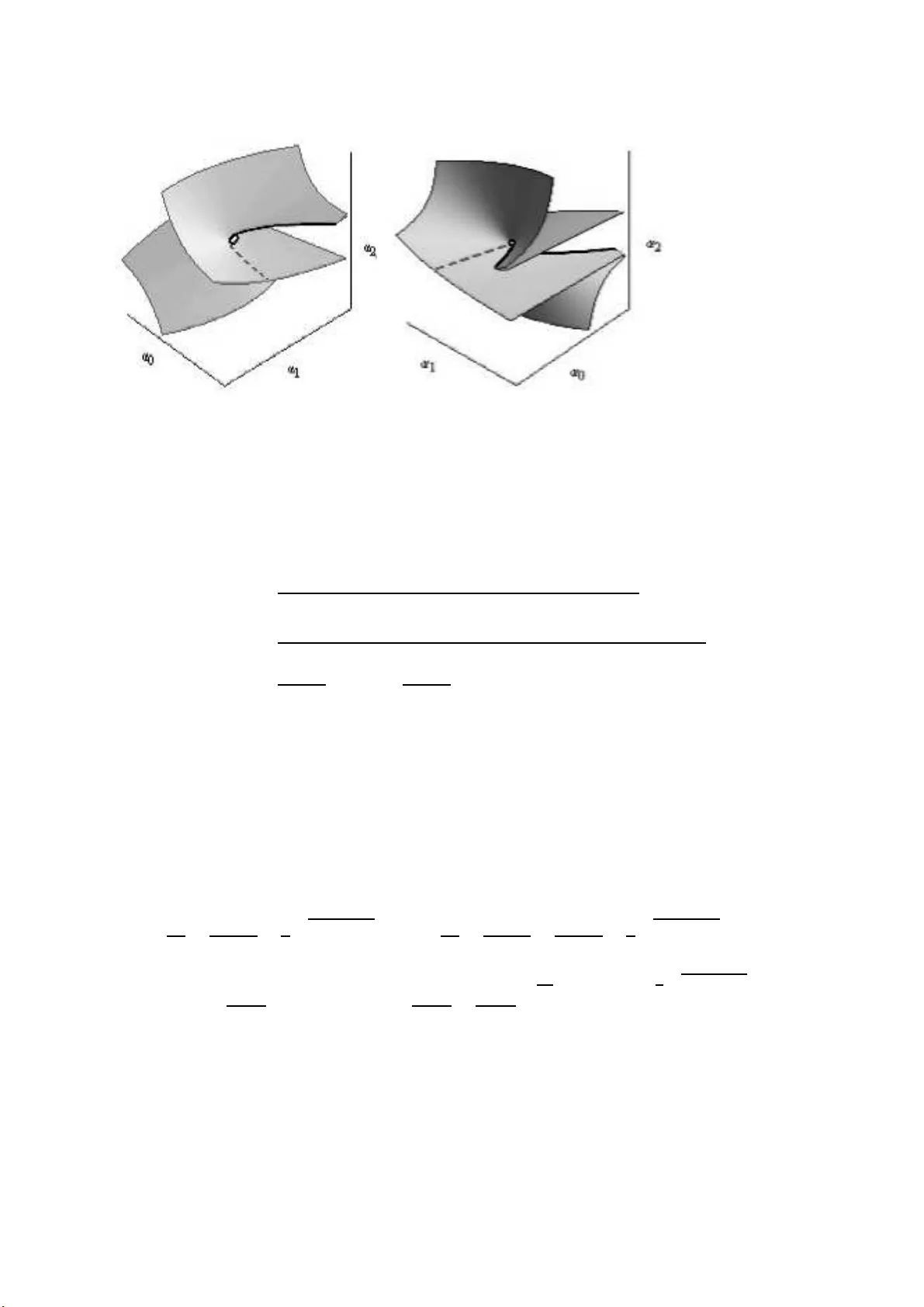
P oisson Y ang-Baxter maps with binomial Lax mat rices Theo doros E. Koulouk as , Departmen t of M a thematics, Univ ersit y of P atras, P atras, GR-265 00 Greece V assili os G. Pap ageorgiou , Departmen t of M a thematics, Univ ersit y of P atras, GR-265 00 P atras, Greece Octob er 24, 201 8 Abstract A construction of mu ltidimensio nal parametric Y ang- Baxter maps is presented. The corres p o nding Lax matrices are the symplectic leaves of first degre e matr ix p olyno mials equipp e d with the Skly anin bracket. These maps ar e symplectic with resp ect t o t he reduced symplectic structure on these lea ves and provide examples of integrable map- pings. An interesting family of quadrir ational sy mplectic YB ma ps on C 4 × C 4 with 3 × 3 Lax matrices is also presented. Con ten ts 1 In tro duction 2 2 Y ang-Baxter Maps and lax matrices 3 3 Symplectic Y ang–B axt er maps associate d to binomial 2 × 2 Lax mat rices 5 3.1 P oisson Y ang–Baxter maps from matrix re-factorization . . . . . . . . . . . 5 3.2 Reduction on symplectic lea v es . . . . . . . . . . . . . . . . . . . . . . . . . 8 3.3 Classification . . . . . . . . . . . . . . . . . . . . . . . . . . . . . . . . . . . 10 3.4 Degenerate YB maps . . . . . . . . . . . . . . . . . . . . . . . . . . . . . . . 12 4 Higher dimensional Y ang-Baxter maps 14 4.1 8-dimensional quadrirational symplectic YB maps with 3 × 3 Lax matrices 16 4.1.1 A 4-parametric symplectic Y-B map . . . . . . . . . . . . . . . . . . 17 4.1.2 The Boussinesq Y-B map ( α 0 = α 3 , α 1 = 3 α 2 , α 2 = 3 α ) . . . . . . . 19 4.1.3 The Goncharenk o–V ese lov map ( α 0 = − α 3 , α 1 = − α 2 , α 2 = α ) . . . 19 5 Conclusion 20 1 1 In tro duc tion Set theoretical solutions o f the qu an tum Y ang-Baxter equation h a ve extensiv ely b een stud ied b y m any authors after the p ioneer w ork of Drinfeld [5]. Ev en b efore that, examples of such solutions app eared in [20] by Sklya n in. W einstein and Xu [24] prop osed a co n struction of suc h solutions using the dressing action of Poi s s on Lie groups [1 8 ]. This wa s generalized later in [11], in order to construct s olutions on an y group that acts on itself and the action satisfies a compatibilit y condition. T he alge b raic asp ects of the Y ang-Baxt er equation we r e dev elop ed b y Etingof, Sc hedler and Solo viev [6 ]. V eselo v [22, 23] connected the set theoretical solutions of the quan tum Y ang-Baxte r equations w ith in tegrable mappings. More sp ecifically , he pro v ed that for su ch a solution, that admits a Lax matrix, there is a hierarch y of comm uting transfer maps whic h pr eserve the sp ectrum o f the corresp onding mono drom y matrix. F u rthermore he prop osed the shorter term ‘Y ang Baxter maps’ for the set theoretical s olutions of the quantum Y ang- Baxter equation. Y ang-Ba xter maps are closely related with in tegrable equations on quad-graphs. This is due to the multidimensional c onsistency pr op erty of these equations, introd uced in [4, 12], whic h in a wa y seems to b e equiv alen t with the Y ang-Baxte r prop erty . An explicit classification of equati ons on quad-graphs with fields in C that satisfy the 3- d imensional consistency prop er ty and of the Y ang-Baxter maps on CP 1 × CP 1 is giv en in [1] and [2] resp ectiv ely (see also [14]). Higher dimensional Y ang-Baxter maps are obtained fr om m ulti- field in tegrable lattice equations thr ough symm etry reduction [15, 16]. Lo op groups equipp ed with the Sklyanin brac k et p ro vide a natur al fr amew ork in order to deriv e Y ang-B axter maps with p olynomial Lax matrices. In [17] one of the most fundamen tal examples of a p arametric Y ang-Baxte r map, Adler’s map, is give n b y Hamiltonian reduction of the lo op group LGL 2 ( R ). Based on these id eas, a construction of P oisson parametric Y ang-Ba xter maps with first deg r ee p olynomial 2 × 2 La x matrices wa s presen ted b y the authors [9] from a r e-factorization p r o cedure guided b y the conserv ation of the Casimir functions un der the maps. By considering a complete set of Casimir functions, sym p lectic m ultiparametric Y ang-Baxter maps were d eriv ed w ith explicit f ormulae in terms of matrix op erations. The purp ose of this w ork is to generalize the metho d of [9] in order to derive sym p lectic Y ang-Ba xter maps with Lax matrices that are obtained by reduction on symplectic lea v es of b inomial matrices. The necessary d efinitions and n otation ab ou t YB maps and L ax m atrices, are giv en in section 2. Section 3 con tains th e main th eory of th e constru ction of sym plectic Y ang-Ba xter maps asso ciated to 2 × 2 Lax m atrices. Th is is generalize d in higher dimensions in section 4 using furth er assumptions. A general r e-factoriza tion f ormula of n × n binomial matrices is present ed. A reduction pro cedure of 3 × 3 binomial matrices to four d imensional symplectic lea v es, pro vid es a family of quadrirational, symplectic YB maps on C 4 × C 4 . Finally we conclude in section 5 by giving some comments and p ersp ectiv es f or future work. 2 2 Y ang-Baxter Maps and lax matrices Let X b e an y set. A map R : X × X → X × X , R : ( x, y ) 7→ ( u ( x, y ) , v ( x, y )), that satisfies the Y ang-Baxter e quation : R 23 R 13 R 12 = R 12 R 13 R 23 (1) is called Y ang-Baxter M ap (YB) [22]. Here b y R ij for i, j = 1 , ..., 3, w e denote the m ap that acts as R on th e i and j facto r of X × X × X and identic ally on the others i.e. R 12 ( x, y , z ) = ( u ( x, y ) , v ( x, y ) , z ) , R 13 ( x, y , z ) = ( u ( x, z ) , y , v ( x, z )) , R 23 ( x, y , z ) = ( x, u ( y , z ) , v ( y , z )) , for x, y , z ∈ X . F rom our p oin t of view, w e consider that the set X has the structure of an algebraic v ariet y . Th e YB map R is calle d non-de gener ate if the maps u ( · , y ) : X → X and v ( x, · ) : X → X are b ijectiv e maps and quadrir ational [2] if they are rational b ijectiv e maps. P arametric YB maps a p p ear in the stud y of in tegrable equations on quad-graphs. A p ar ametric YB ma p is a YB map: R : (( x, α ) , ( y , β )) 7→ (( u, α ) , ( v , β )) = (( u ( x, α, y , β ) , α ) , ( v ( x, α, y , β ) , β )) (2) where x, y ∈ X and the parameters α, β ∈ C n . W e usually k eep the parameters separately and d enote R ( x, α, y , β ) b y R α,β ( x, y ). Acco r ding to [21] a L ax Matrix for the YB map (2) is a matrix L ( x, α, ζ ) th at dep ends on the p oint x , the parameter α and a sp ectral parameter ζ (w e usually denote it just b y L ( x ; α )), such that L ( u ; α ) L ( v ; β ) = L ( y ; β ) L ( x ; α ) , (3) for an y ζ ∈ C . F ur th ermore if equation (3) is equiv alen t to ( u, v ) = R α,β ( x, y ) th en w e will call L ( x ; α ) str ong L ax matrix . A parametric YB map can b e rep r esen ted as a map assigned to the edges of an elemen- tary quadrilateral lik e in Fig.1. ( x ; α ) ( y ; β ) ( u ; α ) ( v ; β ) R α,β Figure 1: A map assigned to the edges of a quadrilateral W e can also represen t the maps R 23 R 13 R 12 and R 12 R 13 R 23 as c hains of maps at the faces of a cub e lik e in Fig.2 . The firs t map co r r esp ond s to th e c omp osition of t h e do wn , b ac k, left faces, while the second one to the right, fron t an d up p er faces. A ll the p arallel edges 3 to the x (resp. y , z ) axis carry the parameter α (resp . β , γ ). If w e denote by ( x ′′ , y ′′ , z ′′ ) and b y ( ˜ ˜ x, ˜ ˜ y , ˜ ˜ z ) the corresp ond ing v alues R 23 R 13 R 12 ( x, y , z ) and R 12 R 13 R 23 ( x, y , z ), then Eq.(1) assures that x ′′ = ˜ ˜ x, y ′′ = ˜ ˜ y and z ′′ = ˜ ˜ z . x y z ˜ z ˜ y ˜ x ˜ ˜ z ˜ ˜ y ˜ ˜ x x y z x ′ y ′ x ′′ z ′ y ′′ z ′′ R 23 R 13 R 12 R 12 R 13 R 23 ( i ) R 23 R 13 R 12 ( ii ) R 12 R 13 R 23 Figure 2: C ubic represent ation of the Y ang–Baxte r prop ert y The fol lowing prop osition [22, 9 ] giv es a sufficien t condition for a solutio n of the L ax equation (3), in order to satisfy th e Y ang-Baxter p rop erty . Prop osition 2.1. L et u = u α,β ( x, y ) , v = v α,β ( x, y ) and A ( x ; α ) a matrix dep ending on a p oint x , a p ar ameter α and a sp e ctr al p ar ameter ζ , such that A ( u ; α ) A ( v ; β ) = A ( y ; β ) A ( x ; α ) . If the e quation A ( ˆ x ; α ) A ( ˆ y ; β ) A ( ˆ z ; γ ) = A ( x ; α ) A ( y ; β ) A ( z ; γ ) (4) implies tha t ˆ x = x, ˆ y = y and ˆ z = z , then the map R α,β ( x, y ) = ( u, v ) is a p ar ametric Y ang-Baxter map with L ax matrix A ( x ; α ) . In a m ore g eneral setting concerning in tegrable lattice s (not necessary YB m aps), instead of the notion of a Lax matrix, th e n otion of a L ax p air is more suitable. A Lax pair for a map Φ α,β : (( x, α ) , ( y, β )) 7→ (( u, α ) , ( v, β )) = (( u ( x, α, y , β ) , α ) , ( v ( x, α, y , β ) , β )) is a pair of matrices L, M dep ending on a p oin t in X , a parameter and a s p ectral parameter ζ suc h that L ( u, α, ζ ) M ( v , β , ζ ) = M ( y , β , ζ ) L ( x, α, ζ ) , (5) for an y ζ ∈ C . Combinations of Lax pairs can provide so lu tions of the en t win ing Y ang- Baxter equation [10]. The d ynamical asp ects of the Y ang-Baxte r maps ha ve b een extensiv ely in vestig ated in [22] and [23] where commuting tr an s fer maps, that pr eserv e the sp ectrum of the corre- sp ond ing mono dromy matrices, are in tro duced for eac h YB map. These maps are b eliev ed to b e inte grable in the Liouville sense, i.e. symplectic mapp ings M 2 n → M 2 n that admit n functionally indep enden t in tegrals in inv olution. 4 3 Symplectic Y ang–Baxter maps asso ciated to binomial 2 × 2 Lax matrices A general matrix re-facto r ization pro cedure provides a w ay of constructing ratio n al multi- parametric Y ang-Baxte r maps on C 4 × C 4 with 2 × 2 Lax matrices in the form of first-degree matrix p olynomials. These maps are Poi s s on with resp ect to the S k lyanin brack et. By reduction on symplectic lea v es we d eriv e 4-dimensional symplectic parametric YB maps. The wh ole pro cedu re generalizes t h e one p resen ted in [9], where the leading terms of the matrix p olynomials w ere assum ed equal. 3.1 P oisson Y ang–Baxter maps from matrix re-factorization W e consider the set L 2 of 2 × 2 p olynomial matrices of the form L ( ζ ) = X − ζ A , ζ ∈ C equipp ed with the Skly anin b rac ke t [19]: { L ( ζ ) ⊗ , L ( η ) } = [ r ζ − η , L ( ζ ) ⊗ L ( η )] , (6) where r denotes the p erm utation matrix: r ( x ⊗ y ) = y ⊗ x . F or X =  x 1 x 2 x 3 x 4  and A =  a 1 a 2 a 3 a 4  , the brac ket s b et wee n the co ordinate fu nctions are giv en by the an tisymmetric P oisson struc- ture matrix : J A ( X ) =     0 − x 2 a 1 + x 1 a 2 x 3 a 1 − x 1 a 3 x 3 a 2 − x 2 a 3 ∗ 0 x 4 a 1 − x 1 a 4 x 4 a 2 − x 2 a 4 ∗ ∗ 0 − x 4 a 3 + x 3 a 4 ∗ ∗ ∗ 0     (7) where J A ( X ) ij = { x i − ζ a i , x j − ζ a j } , for i, j = 1 , ..., 4 . There are six linear indep endent Casimir fun ctions of L 2 whic h are the elemen ts a i , i = 1 , ..., 4, of the matrix A and the fu nctions: f 0 ( X ; A ) = det X , f 1 ( X ; A ) = a 4 x 1 − a 3 x 2 − a 2 x 3 + a 1 x 4 , i.e. the co efficients of the p olynomial p A X ( ζ ) := det ( X − ζ A ) = f 2 ( X ; A ) ζ 2 − f 1 ( X ; A ) ζ + f 0 ( X ; A ) with f 2 ( X ; A ) = det A (of course f 2 ( X ; A ) is also Casimir). F or any constant matrix A w e denote b y i A the im m ersion i A : X 7→ X − ζ A and by L 2 A the lev el set L 2 A = { X − ζ A | X ∈ M at (2 × 2) } . F urthermore for any pair of matrices A, B ∈ GL 2 ( C ), we define the matrix fun ctions Π 1 A,B , Π 2 A,B , with Π 1 A,B ( X, Y ) = f 2 ( X ; A )( Y A + B X ) − f 1 ( X ; A ) AB , (8) Π 2 A,B ( X, Y ) = f 2 ( X ; A ) Y X − f 0 ( X ; A ) AB . (9) 5 Prop osition 3.1. (r e-factorization) L et A, B b e invertible 2 × 2 matric es, su ch that AB = B A and X, Y ∈ M at (2 × 2) with det Π 1 A,B ( X, Y ) 6 = 0 . Then ( U − ζ A )( V − ζ B ) = ( Y − ζ B )( X − ζ A ) , (10) and p A U ( ζ ) = p A X ( ζ ) (e quivalently p B V ( ζ ) = p B Y ( ζ ) ), iff U = U A,B ( X, Y ) := Π 2 A,B ( X, Y )Π 1 A,B ( X, Y ) − 1 A, (11) V = V A,B ( X, Y ) := A − 1 ( Y A + B X − U ( X , Y ) B ) . (12) The pro of of this p rop osition is giv en in [10]. Lemma 1. L et A i , i = 1 , 2 , 3 b e thr e e inv e rtible matric es such that A i A j = A j A i , for i, j = 1 , 2 , 3 . Then ( X ′ 1 − ζ A 1 )( X ′ 2 − ζ A 2 )( X ′ 3 − ζ A 3 ) = ( X 1 − ζ A 1 )( X 2 − ζ A 2 )( X 3 − ζ A 3 ) (13) and p A i X ′ i ( ζ ) = p A i X i ( ζ ) for every X i ∈ M at (2 × 2) , i = 1 , 2 , 3 and ζ ∈ C , iff X ′ 1 = X 1 , X ′ 2 = X 2 X ′ 3 = X 3 . The pro of of this lemma can b e traced in th e app endix of [10]. Prop osition 3.2. L et K : C d → GL 2 ( C ) , b e a d–p ar ametric family of c ommuting matric es. F or every α, β ∈ C d the map R α,β ( X, Y ) = ( U K ( α ) ,K ( β ) ( X, Y ) , V K ( α ) ,K ( β ) ( X, Y )) := ( U, V ) (14) define d by (11), (12), is a p ar ametric Y ang-Baxter map with L ax matrix L ( X ; α ) = i K ( α ) ( X ) such tha t p K ( α ) U ( ζ ) = p K ( α ) X ( ζ ) and p K ( β ) V ( ζ ) = p K ( β ) Y ( ζ ) . Pro of: F o r U = U K ( α ) ,K ( β ) ( X, Y ), V = V K ( α ) ,K ( β ) ( X, Y ) an d L ( X ; α ) = i K ( α ) ( X ), from prop osition 3.1 w e hav e that L ( U ; α ) L ( V ; β ) = L ( Y ; β ) L ( X ; α ) and p K ( α ) U ( ζ ) = p K ( α ) X ( ζ ), p K ( β ) V ( ζ ) = p K ( β ) Y ( ζ ). No w , if w e set R 12 α,β ( X, Y , Z ) = ( X ′ , Y ′ , Z ) , R 13 α,γ ◦ R 12 α,β ( X, Y , Z ) = ( X ′′ , Y ′ , Z ′ ) , R 23 β ,γ ◦ R 13 α,γ ◦ R 12 α,β ( X, Y , Z ) = ( X ′′ , Y ′′ , Z ′′ ) , then L ( Y ; β ) L ( X ; α ) = L ( X ′ ; α ) L ( Y ′ ; β ), and p K ( α ) X ′ ( ζ ) = p K ( α ) X ( ζ ), p K ( β ) Y ′ ( ζ ) = p K ( β ) Y ( ζ ). So L ( Z ; γ ) L ( Y ; β ) L ( X ; α ) = ( L ( Z ; γ ) L ( X ′ ; α )) L ( Y ′ ; β ) = L ( X ′′ ; α )( L ( Z ′ ; γ ) L ( Y ′ ; β )) = L ( X ′′ ; α ) L ( Y ′′ β ) L ( Z ′′ ; γ ) 6 and p K ( α ) X ′′ ( ζ ) = p K ( α ) X ( ζ ) , p K ( β ) Y ′′ ( ζ ) = p K ( β ) Y ( ζ ) , p K ( γ ) Z ′′ ( ζ ) = p K ( γ ) Z ( ζ ) . On th e other hand for R 23 β ,γ ( X, Y , Z ) = ( X , ˜ Y , ˜ Z ) , R 13 α,γ ◦ R 23 β ,γ ( X, Y , Z ) = ( ˜ X , ˜ Y , ˜ ˜ Z ) , R 12 α,β ◦ R 13 α,γ ◦ R 23 β ,γ ( X, Y , Z ) = ( ˜ ˜ X, ˜ ˜ Y , ˜ ˜ Z ) w e get L ( Z ; γ ) L ( Y ; β ) L ( X ; α ) = L ( ˜ ˜ X ; α ) L ( ˜ ˜ Y ; β ) L ( ˜ ˜ Z ; γ ) and p K ( α ) ˜ ˜ X ( ζ ) = p K ( α ) X ( ζ ), p K ( β ) ˜ ˜ Y ( ζ ) = p K ( β ) Y ( ζ ), p K ( γ ) ˜ ˜ Z ( ζ ) = p K ( γ ) Z ( ζ ) . So fin ally we h a v e th at L ( X ′′ ; α ) L ( Y ′′ β ) L ( Z ′′ ; γ ) = L ( ˜ ˜ X ; α ) L ( ˜ ˜ Y ; β ) L ( ˜ ˜ Z ; γ ) , p K ( α ) X ′′ ( ζ ) = p K ( α ) ˜ ˜ X ( ζ ) , p K ( β ) Y ′′ ( ζ ) = p K ( β ) ˜ ˜ Y ( ζ ) , p K ( γ ) Z ′′ ( ζ ) = p K ( γ ) ˜ ˜ Z ( ζ ) and from lemma 1 we derive X ′′ = ˜ ˜ X, Y ′′ = ˜ ˜ Y , Z ′′ = ˜ ˜ Z , i.e. R 23 β ,γ ◦ R 13 α,γ ◦ R 12 α,β = R 12 α,β ◦ R 13 α,γ ◦ R 23 β ,γ . W e will refer to the Y ang-Baxter m ap of Prop. 3.2 as the gener al p ar ametric Y ang- Baxter map asso ciate d with the function K . W e hav e to notice that in general the Lax matrix L ( X ; α ) = i K ( α ) ( X ) is not a strong Lax matrix. F or example by consid er in g K ( α ) = B for a constan t B ∈ GL 2 ( C ), the equation i B ( U ) i B ( V ) = i B ( Y ) i B ( X ) except of the corresp onding solution (11),(12), admits also the trivial solution U = Y , V = X (elemen tary inv olution). No w w e return to the P oisson structure (7). W e can extend the Poisson br ac k et of L 2 to the Cartesian p ro duct L 2 × L 2 as follo ws : { x i , x j } = J A ( X ) ij , { y i , y j } = J B ( Y ) ij , { x i , y j } = 0 , (15) for an y ( X − ζ A, Y − ζ B ) ∈ L 2 × L 2 where x i , x j , y i , y j for i = 1 , ..., 4 are the elemen ts of th e matrices X, Y r esp ectiv ely . Prop osition 3.3. The map R : L 2 K ( α ) × L 2 K ( β ) → L 2 K ( α ) × L 2 K ( β ) , R : ( X − ζ K ( α ) , Y − ζ K ( β )) 7→ ( U K ( α ) ,K ( β ) ( X, Y ) − ζ K ( α ) , V K ( α ) ,K ( β ) ( X, Y ) − ζ K ( β )) (16) is a Poisson map . Pro of: A direct computation of the Poisson br ac k ets of th e elemen ts of U = U K ( α ) ,K ( β ) ( X, Y ) and V = V K ( α ) ,K ( β ) ( X, Y ) defined b y (11), (12) giv es: { u i , u j } = J K α ( U ) ij , { v i , v j } = J K β ( V ) ij , { u i , v j } = 0 , for i = 1 , ..., 4. If w e co n sider the permutatio n map r : ( X , Y ) 7→ ( Y , X ) and t h e m ultiplication map m : ( X, Y ) 7→ X Y , then R is th e unique map d efined b y the comm u tative diagram: 7 L 2 k ( α ) × L 2 k ( β ) r   R / / L 2 k ( α ) × L 2 k ( β ) m   L 2 k ( β ) × L 2 k ( α ) m / / L 2 2 C ommutativ e diag r am Here L 2 2 denotes the second d egree p olynomial 2 × 2 matrices. F rom prop osition 3.3 and the m ultiplication prop erty of the Sklya n in b r ac k et w e conclude that eac h map of this diagram is P oisson. 3.2 Reduction on symplectic lea ves In the p revious section it was p oin ted out that the matrix A of a generic element X − ζ A =  x 1 x 2 x 3 x 4  − ζ  a 1 a 2 a 3 a 4  ∈ L 2 , b elongs to the cen ter of the Sklyanin algebra. I n the four d imensional Po isson subman if old L 2 A there are tw o Casimir fun ctions f 0 ( X ; A ) = det X f 1 ( X ; A ) = a 4 x 1 − a 3 x 2 − a 2 x 3 + a 1 x 4 . W e restrict on the lev el set of the Casimir f unctions by solving the system f 0 ( X ; A ) = α 0 , f 1 ( X ; A ) = α 1 with resp ect to t w o elements x i , x j of X . So w e consider t wo fun ctions h A , g A , defined on an op en set D ⊂ C 4 , suc h that x i = h ( x k , x l , α 0 , α 1 ) and x j = g A ( x k , x l , α 0 , α 1 ) , k , l / ∈ { i, j } . (17) W e denote b y pr k ,l the p ro jection of a matrix to its k , l elemen ts (b y orderin g the elemen ts of a matrix f rom one to f our as b efore) and b y P r the map P r = pr k ,l × p r k ,l : ( X, Y ) 7→ ( pr k ,l ( X ) , pr k ,l ( Y )) . By sub stituting the x i , x j to the m atrix X we define the parametric matrix L ′ A ( x k , x l ; α 0 , α 1 ). F or simp licit y we ren u m b er x k 7→ x 1 , x l 7→ x 2 and w e come up to the matrix L ′ A ( x 1 , x 2 ; α 0 , α 1 ) that satisfies the f ollo wing equations f 0 ( L ′ A ( x 1 , x 2 ; α 0 , α 1 ); A ) = α 0 f 1 ( L ′ A ( x 1 , x 2 ; α 0 , α 1 ); A ) = α 1 . The connected comp onents of Σ A ( α 0 , α 1 ) = { L ′ A ( x 1 , x 2 ; α 0 , α 1 ) − ζ A | x 1 , x 2 ∈ D ⊂ C } are t wo d imensional s ymplectic lea v es of L 2 A . By the next p rop osition th e general YB map R α,β of Prop. 3.2 is r ed uced on the symplectic lea v es Σ K ( α ) ( α 0 , α 1 ) × Σ K ( β ) ( β 0 , β 1 ) of L 2 × L 2 . 8 Prop osition 3.4. L et K : C d 7→ GL 2 ( C ) b e a d–p ar ametric family of c ommuting matric es. F or every α, β ∈ C d , the map R ¯ α, ¯ β (( x 1 , x 2 ) , ( y 1 , y 2 )) = P r ◦ R α,β ( L ′ K ( α ) ( x 1 , x 2 ; α 0 , α 1 ) , L ′ K ( β ) ( y 1 , y 2 ; β 0 , β 1 )) , (18) is a non-de gene r ate symple ctic Y ang-B axter map with ve ctor p ar ameters ¯ α = ( α, α 0 , α 1 ) , ¯ β = ( β , β 0 , β 1 ) ∈ V × C 2 and str ong L ax matrix L ( x 1 , x 2 ; ¯ α ) = i K ( α ) ( L ′ K ( α ) ( x 1 , x 2 ; α 0 , α 1 )) = L ′ K ( α ) ( x 1 , x 2 ; α 0 , α 1 ) − ζ K ( α ) . (19) Pro of: F o r X = L ′ K ( α ) ( x 1 , x 2 ; α 0 , α 1 ) and Y = L ′ K ( β ) ( y 1 , y 2 ; β 0 , β 1 ) we d efine the matrices U = U K ( α ) ,K ( β ) ( X, Y ) , V = V K ( α ) ,K ( β ) ( X, Y )) by (11), (12) ( U, V ) = R α,β ( X, Y ) = R α,β ( L ′ K ( α ) ( x 1 , x 2 ; α, α 0 , α 1 ) , L ′ K ( β ) ( y 1 , y 2 ; β , β 0 , β 1 )) . Since f i ( U ; K ( α )) = f i ( X ; K ( α )) = α i and f i ( V ; K ( β )) = f i ( Y ; K ( β )) = β i for i = 0 , 1, then U = L ′ K ( α ) ( u 1 , u 2 ; α 0 , α 1 ) and V = L ′ K ( β ) ( v 1 , v 2 ; β 0 , β 1 ). The p ro jection P r ( U, V ) giv es the corresp onding elemen ts u = ( u 1 , u 2 ) and v = ( v 1 , v 2 )). So the YB prop erty of the map R ¯ α, ¯ β : (( x 1 , x 2 ; ¯ α ) , ( y 1 , y 2 ; ¯ β )) 7→ (( u 1 , u 2 , ¯ α ) , ( v 1 , v 2 , ¯ β )), is immediately derive d from the YB prop ert y of the P oisson map R α,β . F urthermore p rop osition 3.2 implies that i K ( α ) ( U ) i K ( β ) ( V ) = i K ( β ) ( Y ) i K ( α ) ( X ), so ( L ′ K ( α ) ( u 1 , u 2 ; α 0 , α 1 ) − ζ K α )( L ′ K ( β ) ( v 1 , v 2 ; β 0 , β 1 ) − ζ K β ) = ( L ′ K ( β ) ( y 1 , y 2 ; β 0 , β 1 ) − ζ K β )( L ′ K ( α ) ( x 1 , x 2 ; α 0 , α 1 ) − ζ K α ) (20) whic h means that L ( x 1 , x 2 ; ¯ α ) = L ′ K ( α ) ( x 1 , x 2 ; α 0 , α 1 ) − ζ K α is a Lax matrix for R ¯ α, ¯ β . Also, from prop osition 3.1 we conclud e that L ( x 1 , x 2 ; ¯ α ) is a strong Lax matrix. Finally we notice that equation (20) is d ir ectly solv able with resp ect to v = ( v 1 , v 2 ) and x = ( x 1 , x 2 ), since K − 1 β L ′ K β ( v ; ˆ β ) = ( L ′ K α ( u ; ˆ α ) K β − L ′ K β ( y ; ˆ β ) K α ) − 1 L ′ K β ( y ; ˆ β ) K − 1 β ( L ′ K α ( u ; ˆ α ) K β − L ′ K β ( y ; ˆ β ) K α ) , K − 1 α L ′ K α ( x ; ˆ α ) = ( L ′ K β ( y ; ˆ β ) K α − L ′ K α ( u ; ˆ α ) K β ) − 1 L ′ K α ( u ; ˆ α ) K − 1 α ( L ′ K β ( y ; ˆ β ) K α − L ′ K α ( u ; ˆ α ) K β ) for y = ( y 1 , y 2 ), u = ( u 1 , u 2 ), ˆ α = ( α 0 , α 1 ) and ˆ β = ( β 0 , β 1 ). That p ro ves the n on-degeneracy of th e YB map (18). R emark 3.5 . F rom the construction of the Lax matrix L ( x 1 , x 2 ; ¯ α ) and lemma 1 we can pro ve that the equation: L ( x ′ 1 , x ′ 2 ; ¯ α ) L ( y ′ 1 , y ′ 2 ; ¯ β ) L ( z ′ 1 , z ′ 2 ; ¯ γ ) = L ( x 1 , x 2 ; ¯ α ) L ( y 1 , y 2 ; ¯ β ) L ( z 1 , z 2 ; ¯ γ ) implies x ′ = x, y ′ = y and z ′ = z (with ou t further assumptions). So the YB pr op ert y of the m ap (18) can b e deriv ed directly from Prop. 2.1. R emark 3.6 . If w e set α 0 = β 0 = k on the YB map (18) w e obtain the parametric YB map R ¯ α, ¯ β with parameters ¯ α = ( α, a 1 ) , ¯ β = ( β , b 1 ) ∈ V × C and Lax matrix L ( x 1 , x 2 ; α, α 1 ) := L ( x 1 , x 2 ; α, k , α 1 ). W e ha v e analogous results if w e id en tify any other pair of p arameters. If w e set ¯ α = ¯ β then we derive the trivial solution U = Y , V = X , b ecause this is the only solution of E q .(10 ) with A = B , f 0 ( U ; A ) = f 0 ( Y ; A ) and f 1 ( U ; A ) = f 1 ( Y ; A ). 9 3.3 Classification In this section w e classify the qu adrirational YB maps w ith 2 × 2 binomial Lax matrices of our construction. In [9] a classification b y Jordan normal forms w as giv en for the case K ( α ) = K ( β ) = B , with B a 2 × 2 constant matrix. Here w e giv e a more general classification in order to include all the cases that we considered. First we begin by determining the functions K of prop osition 3.2. Actually w e are going to co n sider the problem of families of commuting m atrices up to conjugation. One can brin g one mem b er of the f amily to its J ordan ca n onical form and find all matrices comm uting with it. F rom this analysis w e conclude that, up to conju gation, there are only tw o (non-disjoint ) famili es of comm u ting pairs of matrices I ) A =  a 1 0 0 a 2  , B =  b 1 0 0 b 2  and I I ) A =  a 1 a 2 0 a 1  , B =  b 1 b 2 0 b 1  . Since the equation (3) and th e YB maps are inv arian t under conju gation w e can restrict to these t wo general cases of the function K : C 2 → GL 2 ( C ). The last step to w ard s th e classification is to examine the relev ance of the choic e of v ariables in the construction of the L ax matrix that w e present ed in the previous section. In the fi rst case, w here K ( α ) is a matrix of the first family for an y α ∈ C 2 , the equations f 0 ( X ; K ( α )) = α 0 , f 1 ( X ; K ( α )) = α 1 (21) are sol v able with resp ect to an y pair ( x i , x j ), for i, j = 1 , ..., 4 , i 6 = j , except of the pair ( x 2 , x 3 ), w hile for a matrix K ( α ) of the second family the equations are solv able with resp ect to an y pair ( x i , x j ), i, j = 1 , ..., 4 , i 6 = j . No w, let us supp ose that, by solving equations (21) in a differen t wa y , we ha v e deriv ed tw o matrices L ′ K ( α ) ( x 1 , x 2 ; α 0 , α 1 ), M ′ K ( α ) ( x ′ 1 , x ′ 2 ; α 0 , α 1 ) suc h that f 0 ( L ′ K ( α ) ( x 1 , x 2 ; α 0 , α 1 ); K ( α )) = α 0 , f 1 ( L ′ K ( α ) ( x 1 , x 2 ; α 0 , α 1 ); K ( α )) = α 1 and f 0 ( M ′ K ( α ) ( x ′ 1 , x ′ 2 ; α 0 , α 1 ); K ( α )) = α 0 , f 1 ( M ′ K ( α ) ( x ′ 1 , x ′ 2 ; α 0 , α 1 )); K ( α )) = α 1 . Then there is a local diffeomorphism φ ¯ α : C 2 → C 2 ( ¯ α = ( α, α 0 , α 1 ) ∈ C 4 ), s u c h that φ ¯ α : ( x 1 , x 2 ) 7→ ( x ′ 1 , x ′ 2 ) and M ′ K ( α ) ( φ ¯ α ( x 1 , x 1 ); α 0 , α 1 ) = L ′ K ( α ) ( x 1 , x 2 ; α 0 , α 1 ) . No w if we denote b y R ¯ α, ¯ β , R ′ ¯ α, ¯ β the parametric YB maps with strong Lax matrices L ( x 1 , x 2 ; ¯ α ) = L ′ K ( α ) ( x 1 , x 2 ; α 0 , α 1 ) − ζ K ( α ) and M ( x ′ 1 , x ′ 2 ; ¯ α ) = M ′ K ( α ) ( x ′ 1 , x ′ 2 ; α 0 , α 1 ) − ζ K ( α ) resp ectiv ely , then ( φ ¯ α × φ ¯ β ) ◦ R ′ ¯ α, ¯ β = R ¯ α, ¯ β ◦ ( φ ¯ α × φ ¯ β ) . (22) F rom the ab ov e analysis w e conclud e that ev ery f our p arametric n on-degenerate YB map on C 2 × C 2 , of p rop osition 3.4, can b e reduced up to equiv alence (22) and reparametrizatio n (see also remark 3.6) into one of the follo win g t wo cases. 10 Case I W e consider the generic element X − ζ K 1 ( α 1 , α 2 ) ∈ L 2 K 1 ( α 1 ,α 2 ) with X =  x 1 x 2 x 3 x 4  and K 1 ( α 1 , α 2 ) =  α 1 0 0 α 2  . The Casimir functions in this case are f 1 ( X ; K 1 ( α 1 , α 2 )) = α 2 x 1 + α 1 x 4 , f 0 ( X ; K 1 ( α 1 , α 2 )) = x 1 x 4 − x 2 x 3 . By setting f 0 ( X ; α 1 , α 2 ) = α 3 , f 1 ( X ; α 1 , α 2 ) = α 4 and solving with r esp ect to x 3 , x 4 , for α 1 , x 2 6 = 0, w e derive the matrix L ′ K 1 ( ˆ α ) ( x 1 , x 2 ; α 3 , α 4 ) = x 1 x 2 x 1 ( α 4 − α 2 x 1 ) − α 1 α 3 α 1 x 2 α 4 − α 2 x 1 α 1 ! with ˆ α = ( α 1 , α 2 ) (23) and the 8-parametric quadrirational YB map of prop osition 3.4 R 1 ¯ α, ¯ β (( x 1 , x 2 ) , ( y 1 , y 2 )) = P r ◦ R 1 ˆ α, ˆ β ( L ′ K 1 ( ˆ α ) ( x 1 , x 2 ; α 3 , α 4 ) , L ′ K 1 ( ˆ β ) ( y 1 , y 2 ; β 3 , β 4 )) . Here R 1 ˆ α, ˆ β is the general p arametric YB map (14) asso ciated with the function K 1 , the pro jection P r = pr 1 , 2 × pr 1 , 2 (pro jections at the elemen ts of the first arro w of a mat r ix) and the p arameters are ¯ α = ( α 1 , α 2 , α 3 , α 4 ), ¯ β = ( β 1 , β 2 , β 3 , β 4 ). According to prop. 3.4 , this map ad m its the strong Lax matrix L 1 ( x 1 , x 2 ; ¯ α ) = L ′ K 1 ( ˆ α ) ( x 1 , x 2 ; α 3 , α 4 ) − ζ K 1 ( α 1 , α 2 ) , and for α 1 , β 1 6 = 0 it is a symp lectic rational map on { ( x 1 , x 2 ) , ( y 1 , y 2 ) ∈ C 2 × C 2 | x 2 , y 2 6 = 0 } , with resp ect to th e reduced symplectic form defined b y the brack ets: { x 1 , x 2 } = − α 1 x 2 , { y 1 , y 2 } = − β 1 y 2 , { x i , y j } = 0 for i = 1 , 2 . Case I I F or K 2 ( α 1 , α 2 ) =  α 1 α 2 0 α 1  w e set again f 0 ( X ; K 2 ( α 1 , α 2 )) = α 3 , f 1 ( X ; K 2 ( α 1 , α 2 )) = α 4 and solv e with resp ect to to x 3 , x 4 to get L ′ K 2 ( ˆ α ) ( x 1 , x 2 ; α 3 , α 4 ) = x 1 x 2 α 4 x 1 − α 1 ( x 1 2 + α 3 ) α 1 x 2 − α 2 x 1 α 2 α 3 − α 4 x 2 + α 1 x 1 x 2 α 2 x 1 − α 1 x 2 ! , with ˆ α = ( α 1 , α 2 ) (24) and the corresp onding YB map R 2 ¯ α, ¯ β (( x 1 , x 2 ) , ( y 1 , y 2 )) = P r ◦ R 2 ˆ α, ˆ β ( L ′ K 2 ( ˆ α ) ( x 1 , x 2 ; α 3 , α 4 ) , L ′ K 2 ( ˆ β ) ( y 1 , y 2 ; β 3 , β 4 )) , with ¯ α = ( α 1 , α 2 , α 3 , α 4 ) , ¯ β = ( β 1 , β 2 , β 3 , β 4 ) , P r = pr 1 , 2 × pr 1 , 2 and R 2 ˆ α, ˆ β the gen- eral parametric YB map associated with K 2 . This map admits th e strong Lax matrix 11 L 2 ( x 1 , x 2 ; ¯ α ) = L ′ K 2 ( ˆ α ) ( x 1 , x 2 ; α 3 , α 4 ) − ζ K 2 ( α 1 , α 2 ). The reduced Skly anin brac ket in this case is giv en by brac kets of the co ord inates { x 1 , x 2 } = α 2 x 1 − α 1 x 2 , { y 1 , y 2 } = β 2 y 1 − β 1 y 2 , { x i , y j } = 0 for i, j = 1 , 2 . As it was pointed out, YB maps with less parameters can b e co n structed from these t wo cases by setting α i = β i = k f or some i ∈ { 1 , 2 } . Also, b y using appropriate scalings, one can reduce the n u m b er of parameters. Ho wev er, we d o not do this here, ha ving in mind degenerate ca ses in sub section 3.4 b elo w, as we ll as consideration of con tinuous limits in the f uture. Remark. If we ar e inter e ste d in r e al L ax matric es we ha ve to include als o t he c ase wher e K 3 ( α 1 , α 2 ) =  α 1 − α 2 α 2 α 1  and the c orr esp onding YB map of pr op osition 3.4. 3.4 Degenerate YB map s Degenerate YB maps can arise w hen K ( α ) is not inv ertible. A wa y of constru cting degener- ate YB map s as limits of the non-degenerate ones w as presented in [9] f or K ( α ) = K ( β ) = C onstant . W e will apply this metho d here as w ell for K ( α ) 6 = K ( β ). W e consider a fun ction K : V → GL 2 ( C ), V ⊂ C 4 , d ep endin g fr om a parameter ε , suc h that K ( α, ε ) K ( β , ε ) = K ( β , ε ) K ( α, ε ) and lim ε → 0 det K ( α, ε ) = 0 for ev ery α, β ∈ C m , m ≤ 4. W e construct th e corresp ond ing non-degenerate YB m ap R ¯ α, ¯ β ( ε ) of pr op osition 3.4. Th e limit o f R ¯ α, ¯ β ( ε ), for ε → 0, ca n lead to a r ational dege n erate YB map on C 2 × C 2 . The induced Poisson structure is defined by the limit of the S kly anin brac k et. W e apply this construction in the n ext concrete example. A generalization of t he Adler-Y amilo v map W e consider the function K : C → GL 2 ( C ) with K ( α 1 ) = K α 1 =  α 1 0 0 ε  . The Casimir functions on L 2 K ( α 1 ) are : f 0 ( X ; K ( α 1 )) = x 11 x 22 − x 12 x 21 , f 1 ( X ; K ( α 1 )) = εx 11 + α 1 x 22 . (Here we denote b y x ij the elemen ts of the matrix X ). If we set f 0 ( X ; K ( α 1 )) = α 2 , f 1 ( X ; K ( α 1 )) = α 3 and solve with r esp ect to x 11 , x 22 w e hav e x 11 = 1 2 ε ( α 3 − ( α 2 3 − 4 α 1 ε ( α 2 + x 12 x 21 )) 1 / 2 ) , x 22 = 1 2 α 1 ( α 3 + ( α 2 3 − 4 α 1 ε ( α 2 + x 12 x 21 )) 1 / 2 ) . By su bstituting this v alues to X − ζ K ( α 1 ) and ren aming x 12 , x 21 as x 1 and x 2 resp ectiv ely , w e obtain the three-parametric Lax matrix L ( x 1 , x 2 ; ¯ α ) = α 3 − ( α 2 3 − 4 α 1 ε ( α 2 + x 1 x 2 )) 1 / 2 2 ε − α 1 ζ x 1 x 2 α 3 +( α 2 3 − 4 α 1 ε ( α 2 + x 1 x 2 )) 1 / 2 2 α 1 − εζ ! (25) 12 with ¯ α = ( α 1 , α 2 , α 3 ), of the n on-degenerate YB m ap of prop osition 3.4 R ¯ α, ¯ β (( x 1 , x 2 ) , ( y 1 , y 2 )) = (( u 1 , u 2 ) , ( v 1 , v 2 )) . (26) Here u 1 , u 2 , v 1 , v 2 are the corresp ondin g elemen ts u 12 , u 21 , v 12 , v 21 of the matrices: [ u ij ] := U = ( α 1 εY X − α 2 K α 1 K β 1 )(( α 1 ε ( Y K α 1 + K β 1 X ) − α 3 K α 1 K β 1 ) − 1 K α 1 [ v ij ] := V = K − 1 α 1 ( Y K α 1 + K β 1 X − U K β 1 ) , for X = L ′ K ( α 1 ) ( x 1 , x 2 ; ¯ α ) ≡ L ( x 1 , x 2 ; ¯ α ) + ζ K α and Y = L ′ K ( α 1 ) ( y 1 , y 2 ; ¯ β ) ≡ L ( y 1 , y 2 ; ¯ β ) + ζ K β . The limit of (26), f or ε → 0, giv es the degenerate 6-parametric Y ang-Baxter map ˜ R ¯ α, ¯ β (( x 1 , x 2 ) , ( y 1 , y 2 )) = (( ¯ u 1 , ¯ u 2 ) , ( ¯ v 1 , ¯ v 2 )) , where ¯ u 1 = β 1 α 1 β 3 ( α 3 y 1 − Qx 1 ) , ¯ u 2 = α 1 β 1 y 2 , ¯ v 1 = β 1 α 1 x 1 , ¯ v 2 = α 1 β 1 α 3 ( β 3 x 2 − Qy 2 ) , and Q = α 1 β 1 ( α 2 β 3 − α 3 β 2 ) α 3 β 3 + α 1 β 1 x 1 y 2 . This map is symplectic with resp ect to th e symplectic form obtained b y taking the li m it, for ε → 0, of J K α ( L ′ ( x 1 , x 2 ; ¯ α )) and J K α ( L ′ ( y 1 , y 2 ; ¯ β )), { x 1 , x 2 } = α 3 , { y 1 , y 2 } = β 3 , { x i , y j } = 0 , (27) and admits the strong Lax matrix M ( x 1 , x 2 ; ¯ α ) = lim ε → 0 L ( x 1 , x 2 ; ¯ α ) =  α 1 α 3 ( α 2 + x 1 x 2 ) − α 1 ζ x 1 x 2 α 3 α 1  . If we set α 3 = β 3 = 1 on the m ap ˜ R ¯ α, ¯ β w e deriv e th e 4-parametric YB map ˜ R ( α 1 ,α 2 ) , ( β 1 ,β 2 ) with strong Lax matrix M ( x 1 , x 2 ; α 1 , α 2 , 1). The induced symplectic form in this c ase is the ca n onical one. Moreo v er by setting α 1 = β 1 = α 3 = β 3 = 1, ¯ R ¯ α, ¯ β is reduced to the Adler-Y amilo v map [3, 9]. According t o [13, 10] the mono drom y matrix of the 1-p erio d ic ‘sta ircase’ initial v alue problem on a qu adrilateral lattice is M 1 ( x 1 , x 2 , y 1 , y 2 ) ≡ M ( y 1 , y 2 ; ¯ β ) M ( x 1 , x 2 ; ¯ α ). The trace of the mono dromy matrix giv es the t wo functionally indep end en t in tegrals : J 1 ( x 1 , x 2 , y 1 , y 2 ) = α 1 β 1 α 3 x 1 x 2 + α 1 β 1 β 3 y 1 y 2 J 2 ( x 1 , x 2 , y 1 , y 2 ) = x 2 y 1 + x 1 y 2 + α 1 β 1 α 3 β 3 ( α 2 + x 1 x 2 )( β 2 + y 1 y 2 ) . W e can verify that these in tegrals are in in v olution with resp ect to (27). So w e conclude that th e map ˜ R ¯ α, ¯ β (( x 1 , x 2 ) , ( y 1 , y 2 )) 7→ (( ¯ u 1 , ¯ u 2 ) , ( ¯ v 1 , ¯ v 2 )) is integrable in the Liouville sense. F or the Adler-Y amilo v map the corresp ond ing in tegrals are giv en by setting α 1 = β 1 = α 3 = β 3 = 1 in J 1 and J 2 . 13 4 Higher dimensional Y ang-Baxter maps In order to generate higher dimen s ional Y ang-Baxter maps we consider the set L n of n order p olynomial matrices of the form X − ζ A . There are n ( n + 1) fu nctionally indep en den t Casimir functions on L n with resp ect to th e S kly anin b rac k et (6 ), whic h are again the n 2 elemen ts of A and th e n fun ctions f i , i = 0 , ..., n − 1, defined as the co efficien ts of the p olynomial p A X ( ζ ) = det ( X − ζ A ), p A X ( ζ ) = ( − 1) n f n ( X ; A ) ζ n + ( − 1) n − 1 f n − 1 ( X ; A ) ζ n − 1 + ... + ( − 1) f 1 ( X ; A ) ζ + f 0 ( X ; A ) where f n ( X ; A ) = detA and f 0 ( X ; A ) = detX . As in the 2 × 2 case, w e consider K : C d → GL n ( C ) a d –parametric family of commuting matrices. Next, for α ∈ C d , we denote the v alue K ( α ) by K α and the v alues of the Casimirs f i ( X ; K ( α )) by f i ( X ; α ), i = 0 , ..., n . Prop osition 4.1. L et U and V b e n × n matric es that satisfy the fol lowing two c onditions (i) f i ( U ; α ) = f i ( X ; α ) a nd f i ( V ; β ) = f i ( Y ; β ) for i = 0 , ..., n − 1 , (ii) ( U − ζ K α )( V − ζ K β ) = ( Y − ζ K β )( X − ζ K α ) , identic al ly in ζ ∈ C for X , Y ∈ M at ( n × n ) suc h that det P n i =1 ( − 1) i f i ( X ; α ) M i − 1 6 = 0 } . Then U = − f 0 ( X ; α ) I − n X i =1 ( − 1) i f i ( X ; α ) N i − 1 ! n X i =1 ( − 1) i f i ( X ; α ) M i − 1 ! − 1 K α (28) V = K − 1 α ( Y K α + K β X − U K β ) , (29) wher e M i , N i ar e give n by: M 0 = I , N 0 = 0 , M 1 = ( Y K α + K β X ) K − 1 β K − 1 α , N 1 = − Y X K − 1 β K − 1 α , M i = M 1 M i − 1 + N i − 1 , N i = N 1 M i − 1 , f or i = 2 , ..., n. Pro of: Since f i ( U ; α ) = f i ( X ; α ), for i = 1 , ..., n , th en p K α U ( ζ ) = p K α X ( ζ ). Ca yley-Hamilt on theorem states that p K α U ( U K − 1 α ) = p K α X ( U K − 1 α ) = 0. So n X i =1 ( − 1) i f i ( X ; α )( U K − 1 α ) i = − f 0 ( X ; α ) I , i = 1 , ..., n. (30) F urthermore from ( ii ) w e derive the system: U V = Y X , U K β + K α V = Y K α + K β X (31) whic h implies ( U K − 1 α ) 2 = U K − 1 α ( Y K α + K β X ) K − 1 β K − 1 α − Y X K − 1 β K − 1 α . (32) 14 F or simplicit y w e s et ˜ U = U K − 1 α , M 1 = ( Y K α + K β X ) K − 1 β K − 1 α and N 1 = − Y X K − 1 β K − 1 α . So equation (32) can b e written as ˜ U 2 = ˜ U M 1 + N 1 . Also if w e se t M 0 = I , N 0 = 0 and define M i , N i from the r ecurrence relations: M i = M 1 M i − 1 + N i − 1 , N i = N 1 M i − 1 f or i = 1 , ..., n, (33) then we can ev aluate the p ow ers of ˜ U k as ˜ U k = ˜ U M k − 1 + N k − 1 for k = 1 , ..., n . So equation (30) b ecomes: n X i =1 ( − 1) i f i ( X ; α )( ˜ U M i − 1 + N i − 1 ) = − f 0 ( X ; α ) I , and finally w e hav e ˜ U = − f 0 ( X ; α ) I − n X i =1 ( − 1) i f i ( X ; α ) N i − 1 ! n X i =1 ( − 1) i f i ( X ; α ) M i − 1 ! − 1 So U = ˜ U K α and from(31) V = K − 1 α ( Y K α + K β X − U K β ) . R emark 4.2 . If w e write the fi rst equ ation of (31) as U K − 1 α K α V = Y X and replace K α V from the second one, we get that U K − 1 α ( Y K α − U K β ) = ( Y K α − U K β ) K − 1 α X. In a similar w a y w e can show that ( U K β − Y K α ) K − 1 β V = Y K − 1 β ( U K β − Y K α ). So if det( U K β − Y K α ) 6 = 0 (equiv alen tly det( K α V − K β X ) 6 = 0 sin ce U K β − Y K α = K α V − K β X ) then the matrice s U K − 1 α , K − 1 β V are similar with the matrices K − 1 α X and Y K − 1 β resp ectiv ely , and subsequently p K α U ( ζ ) = p K α X ( ζ ) , p K β V ( ζ ) = p K β Y ( ζ ). Therefore th e condition ( i ) of prop osition 4.1 can b e replaced b y the assu m ption d et( U K β − Y K α ) 6 = 0 (equiv alen tly det( K α V − K β X ) 6 = 0). R emark 4.3 . Prop osition 4.1 holds also if w e replace K α , K β b y t wo in ve r tible matrices A and B resp ectiv ely suc h that AB = B A . Th e reason f or restricting to the fu nction K is that w e are in terested to consider L ( X ; α ) = X − ζ K α as a Lax matrix of a YB map, otherwise we would ha v e a Lax pair L ( X ; A ) = X − ζ A, M ( Y ; B ) = Y − ζ B with L 6 = M as in [10]. The Y ang-Ba xter prop ert y of th is re-factoriz ation solution, i.e. of the map R α,β ( X, Y ) 7→ ( U, V ) , with U, V defined b y (28) and (29), is still an op en problem. In lo w dimensions, for certain c hoices of th e fun ction K , this can b e c hec ked b y direct computation or by prop osition 2.1. W e conjecture that this is true for any dimension. Anyw a y , since f i ( U ; α ) = f i ( X ; α ) and f i ( V ; β ) = f i ( Y ; β ), the map R α,β can b e reduced, as in 2 × 2 case, to a map on C n ( n − 1) × C n ( n − 1) b y the restriction to the corresp onding lev el s ets of the n Casimir f u nctions f i , i = 0 , ..., n − 1. F urther reduction on lo wer dimen sional symplectic lea v es is also p ossible. 15 4.1 8-dimensional quadrirational symplectic YB maps with 3 × 3 Lax matrices In the case of L 3 there exist three Casimir functions, s o the map of Prop.4.1 can b e redu ced to a qu adrirational map on C 6 × C 6 . F urther reduction to four dimensional symplectic submanifolds of L 3 pro vid e maps on C 4 × C 4 . Ne xt, we demonstrate this pro cedu re for K α = K β = I . Let L ( ζ ) = X − ζ I , with X = [ x ij ], b e a generic elemen t of L 3 I . In this case the S kly anin brac k et is { L ( ζ ) ⊗ , L ( η ) } = [ r ζ − η , L ( ζ ) ⊗ L ( η )] =               0 − x 12 − x 13 x 12 0 0 x 13 0 0 x 21 0 0 x 22 − x 11 − x 12 − x 13 x 23 0 0 x 31 0 0 x 32 0 0 x 33 − x 11 − x 12 − x 13 − x 21 x 11 − x 22 − x 23 0 x 12 0 0 x 13 0 0 x 21 0 − x 21 0 − x 23 0 x 23 0 0 x 31 0 0 x 32 0 − x 21 x 33 − x 22 − x 23 − x 31 − x 32 x 11 − x 33 0 0 x 12 0 0 x 13 0 0 x 21 − x 31 − x 32 x 22 − x 33 0 0 x 23 0 0 x 31 0 0 x 32 − x 31 − x 32 0               (34) Generically the rank of the structure matrix (34 ) is six. W e are inte r ested in finding 4- dimensional symp lectic subm an if olds of L 3 I . F or this r eason we would like to fi nd conditions suc h that the rank of the matrix (34) drops d o wn to four. Let i 1 < ... < i 6 , j 1 < ... < j 6 , with i k , j k ∈ { 1 , .. ., 9 } for k = 1 , ... , 6. W e d enote by m (( i 1 , ..., i 6 ) , ( j 1 , ...j 6 )) the sixth order minor of the matrix (34), consisting of the i 1 , ..., i 6 ro ws and the j 1 , ..., j 6 columns. Using th is notation we p ro ve the next lemma. Lemma 2. Consider the system of e quations obtaine d b y setting al l sixth or der minors m (( i 1 , ..., i 6 ) , ( j 1 , ...j 6 )) e qual to zer o. Ther e is a unique solution of this system with r esp e ct to x 11 , x 31 , x 32 , for nonzer o x 13 , x 23 , namely: x 11 = x 13 x 21 x 23 + x 22 − x 12 x 23 x 13 , x 31 = x 21 ( x 12 x 23 + x 13 ( x 33 − x 22 )) x 13 x 23 , x 32 = x 12 ( x 12 x 23 + x 13 ( x 33 − x 22 )) x 13 2 . (35) Substituting these values to X − ζ I the r ank o f the Poisson matrix in (34) r e duc es to four and the Casimirs f 0 ( X ; I ) := α 0 , f 1 ( X ; I ) := α 1 , f 2 ( X ; I ) := α 2 satisfy 4 α 0 α 2 3 − α 1 2 α 2 2 + 4 α 1 3 − 18 α 0 α 1 α 2 + 27 α 0 2 = 0 (36) Pro of: Consider the minors m 1 = m ((1 , 2 , 3 , 4 , 5 , 6) , (3 , 4 , 6 , 7 , 8 , 9)) = −  x 21 x 2 13 − x 11 x 23 x 13 + x 22 x 23 x 13 − x 12 x 2 23  2 , m 2 = m ((1 , 2 , 3 , 4 , 6 , 7) , (3 , 4 , 5 , 6 , 8 , 9)) = −  x 23 x 2 12 − x 13 x 22 x 12 + x 13 x 33 x 12 − x 2 13 x 32  2 , m 3 = m ((1 , 2 , 3 , 5 , 6 , 9) , (1 , 2 , 3 , 5 , 6 , 9)) = − ( x 12 x 23 x 31 − x 13 x 21 x 32 ) 2 . 16 Figure 3: Tw o views of surf ace (36) in R 3 , b lac k cur v e: ( α 3 , 3 α 2 , 3 α ), dashed curve: ( − α 3 , − α 2 , α ) The sys tem m 1 = m 2 = m 3 = 0 is linear with resp ect to x 11 , x 31 , x 32 and for x 13 , x 23 6 = 0 admits the unique solution (35 ). Su bstituting these v alues to (34) the rank redu ces to four and the C asimir functions b ecome: f 0 ( X ; I ) = ( x 13 x 22 − x 12 x 23 ) 2  x 21 x 2 13 + x 23 x 33 x 13 + x 12 x 2 23  x 3 13 x 23 f 1 ( X ; I ) = ( x 13 x 22 − x 12 x 23 )  2 x 21 x 2 13 + x 23 ( x 22 + 2 x 33 ) x 13 + x 12 x 2 23  x 2 13 x 23 (37) f 2 ( X ; I ) = x 13 x 21 x 23 + 2 x 22 − x 12 x 23 x 13 + x 33 . whic h satisfy (36). It is remark able that t wo curv es on the surface (36) giv e rise to maps related to the Boussinesq and the matrix K dV equation. 4.1.1 A 4-parametric symplectic Y-B map If we set the v alues (35) to X , in ord er to restrict on the lev el sets of the Casimir functions of L 3 I w e set f 2 ( X ; I ) = α 2 , f 1 ( X ; I ) = α 1 (of course f 0 ( X ; I ) will b e also constant since (36) m ust b e satisfied) and solv e (37) with resp ect to x 22 and x 33 to get x 22 = α 2 3 + x 12 x 23 x 13 ± 1 3 q α 2 2 − 3 α 1 , x 33 = α 2 3 − x 13 x 21 x 23 − x 12 x 23 x 13 ∓ 2 3 q α 2 2 − 3 α 1 . F or simplicit y we can change the p arameters in to c 1 = α 2 3 and c 2 = ± 1 3 p α 2 2 − 3 α 1 , so x 22 = c 1 + c 2 + x 12 x 23 x 13 , x 33 = c 1 − 2 c 2 − x 13 x 21 x 23 − x 12 x 23 x 13 . Sub s tituting th ese v alues to (35) and the n ew x ij to X − ζ I , w e obtain the t wo p arametric family of matrices 17 M ( x 12 , x 13 , x 21 , x 23 ; c 1 , c 2 ) =    x 13 x 21 x 23 + c 1 + c 2 − ζ x 12 x 13 x 21 x 12 x 23 x 13 + c 1 + c 2 − ζ x 23 − x 13 x 2 21 x 2 23 − 3 c 2 x 21 x 23 − x 12 x 21 x 13 − x 23 x 2 12 x 2 13 − 3 c 2 x 12 x 13 − x 21 x 12 x 23 c 1 − 2 c 2 − x 13 x 21 x 23 − x 12 x 23 x 13 − ζ    (38) The reduced Poisson structure is { x 12 , x 21 } = x 12 x 23 x 13 − x 13 x 21 x 23 , { x 12 , x 23 } = − x 13 , { x 13 , x 21 } = x 23 and { x 12 , x 13 } = { x 13 , x 23 } = { x 21 , x 23 } = 0, w h ic h defines the symplectic form : ω = 1 x 23 dx 13 ∧ dx 21 − 1 x 13 dx 12 ∧ dx 23 + ( x 12 x 2 13 − x 21 x 2 23 ) dx 13 ∧ dx 23 . W e can change to canonical v ariables by setting x 13 = X 1 , x 23 = X 2 , x 21 = − x 1 X 2 , x 12 = − x 2 X 1 . (39) Then w e denote matrix M ( x 12 , x 13 , x 21 , x 23 ; c 1 , c 2 ) b y L ( x 1 , x 2 , X 1 , X 2 ; c 1 , c 2 ) ≡ L ′ I ( x 1 , x 2 , X 1 , X 2 ; α 1 , α 2 ) − ζ I ≡   c 1 + c 2 − x 1 X 1 − ζ − X 1 x 2 X 1 − x 1 X 2 c 1 + c 2 − x 2 X 2 − ζ X 2 − x 1 ( x 1 X 1 + x 2 X 2 − 3 c 2 ) − x 2 ( x 1 X 1 + x 2 X 2 − 3 c 2 ) c 1 − 2 c 2 + x 1 X 1 + x 2 X 2 − ζ   (40) and the s y m plectic form ω b y the canonical symplectic form ω 0 = dx 1 ∧ dX 1 + dx 2 ∧ dX 2 . F rom th e re-factorization form u la (28), (29), for K α = K β = I , X = L ′ I ( x 1 , x 2 , X 1 , X 2 ; α 1 , α 2 ) and Y = L ′ I ( y 1 , y 2 , Y 1 , Y 2 ; β 1 , β 2 ), since the C asimir functions on Σ I ( α 1 , α 2 ) = { L ( x 1 , x 2 , X 1 , X 2 ; α 1 , α 2 ) | x 1 , x 2 , X 1 , X 2 ∈ C } are f 0 ( X ; I ) = ( α 1 − 2 α 2 )( a 1 + a 2 ) 2 , f 1 ( X ; I ) = 3( α 2 1 − α 2 2 ) , f 2 ( X ; I ) = 3 α 1 , w e obtain the matrices U = ( Y X (3 α 1 I − Y − X ) − ( α 1 − 2 α 2 )( a 1 + a 2 ) 2 I )((3 α 1 I − Y − X )( Y + X )+ Y X − 3( α 2 1 − α 2 2 ) I ) − 1 , V = Y + X − U . If w e d enote b y U ij , V ij the elemen ts of th e matrices U an d V , w e come up to the next prop osition. Prop osition 4.4. The map R (( α 1 ,α 2 ) , ( β 1 ,β 2 )) : (( x 1 , x 2 , X 1 , X 2 ) , ( y 1 , y 2 , Y 1 , Y 2 )) 7→ (( u 1 , u 2 , U 1 , U 2 ) , ( v 1 , v 2 , V 1 , V 2 )) wher e U 1 = U 13 , U 2 = U 23 , u 1 = − U 21 U 23 , u 2 = − U 12 U 13 , V 1 = V 13 , V 2 = V 23 , v 1 = − V 21 V 23 , v 2 = − V 12 V 13 is a symple ctic p ar ametric Y ang-Baxter map, with r esp e ct to the c anonic al symple ctic form dx 1 ∧ dX 1 + dx 2 ∧ dX 2 + dy 1 ∧ d Y 1 + dy 2 ∧ d Y 2 , and admits the str ong L ax matrix L ( x 1 , x 2 , X 1 , X 2 ; α 1 , α 2 ) . 18 Pro of: The YB prop ert y of this map can b e c hec k ed by direct co mp utation. Moreo v er u i , U i , v i , V i , i = 1 , 2 is the un ique solution (pr op osition 4.1) of th e Lax equ ation: L ( u 1 , u 2 , U 1 , U 2 ; α 1 , α 2 ) L ( v 1 , v 2 , V 1 , V 2 ; β 1 , β 2 ) = L ( y 1 , y 2 , Y 1 , Y 2 ; β 1 , β 2 ) L ( x 1 , x 2 , X 1 , X 2 ; α 1 , α 2 ) The explicit form u la of th e YB map R (( α 1 ,α 2 ) , ( β 1 ,β 2 )) of prop osition 4.4 is ( u 1 , u 2 ) = ( y 1 , y 2 ) − α 1 − β 1 − 2( α 2 − β 2 ) D ( x 1 − y 1 , x 2 − y 2 ) , ( v 1 , v 2 ) = ( x 1 , x 2 ) + α 1 − β 1 + α 2 − β 2 D ( x 1 − y 1 , x 2 − y 2 ) , with D = 2 α 2 − α 1 + β 1 + β 2 + y 1 X 1 + y 2 X 2 − x 1 X 1 − x 2 X 2 , and U 1 = ( x 1 − v 1 ) X 1 + ( y 1 − v 1 ) Y 1 u 1 − v 1 , U 2 = ( x 2 − v 2 ) X 2 + ( y 2 − v 2 ) Y 2 u 2 − v 2 , V 1 = ( x 1 − u 1 ) X 1 + ( y 1 − u 1 ) Y 1 v 1 − u 1 , V 2 = ( x 2 − u 2 ) X 2 + ( y 2 − u 2 ) Y 2 v 2 − u 2 . W e will p oint o u t t w o s p ecial cases of this Y B map that giv e rise to Boussinesq and Gonc harenko –V eselo v maps. 4.1.2 The Boussinesq Y-B map ( α 0 = α 3 , α 1 = 3 α 2 , α 2 = 3 α ) By setting c 2 = 0 , c 1 = α to (40) w e derive the Lax matrix L B ( x 1 , x 2 , X 1 , X 2 ; α ) =   α − ζ − x 1 X 1 − X 1 x 2 X 1 − x 1 X 2 α − ζ − x 2 X 2 X 2 − x 1 ( x 1 X 1 + x 2 X 2 ) − x 2 ( x 1 X 1 + x 2 X 2 ) α − ζ + x 1 X 1 + x 2 X 2   In this case th e Casimir functions on Σ I ( α ) = { L B ( x 1 , x 2 , X 1 , X 2 ; α ) / x 1 , x 2 , X 1 , X 2 ∈ C } are f 0 ( X ; I ) = α 3 , f 1 ( X ; I ) = 3 α 2 , f 2 ( X ; I ) = 3 α, for X = L B I ( x 1 , x 2 , X 1 , X 2 ; α ) ≡ L B ( x 1 , x 2 , X 1 , X 2 ; α ) + ζ I . Th e cur ve ( α 3 , 3 α 2 , 3 α ) is depicted in fig. 3 with blac k co lor. The corr esp onding 2-parametric YB m ap R B α,β with s tr ong Lax matrix L B ( x 1 , x 2 , X 1 , X 2 ; c ) is induced from the YB map R (( α 1 ,α 2 ) , ( β 1 ,β 2 )) of prop osition 4.1 i.e. R B α,β = R (( α, 0) , ( β, 0)) . 4.1.3 The Gonc ha renk o–V eselo v map ( α 0 = − α 3 , α 1 = − α 2 , α 2 = α ) In a similar wa y if we set c 1 = α 3 and c 2 = 2 α 3 w e obtain the Y ang-Baxte r map R GV α,β = R (( α 3 , 2 α 3 ) , ( β 3 , 2 β 3 )) with strong Lax m atrix L GV ( x ; α ) =   α − ζ − x 1 X 1 − X 1 x 2 X 1 − x 1 X 2 α − ζ − x 2 X 2 X 2 − x 1 ( x 1 X 1 + x 2 X 2 − 2 α ) − x 2 ( x 1 X 1 + x 2 X 2 − 2 α ) x 1 X 1 + x 2 X 2 − α − ζ   19 for x = ( x 1 , x 2 , X 1 , X 2 ). Here for X = L GV ( x ; α ) + ζ I , ( f 0 ( X ; I ) , f 1 ( X ; I ) , f 2 ( X ; I )) = ( − α 3 , − α 2 , α ), which is the dashed curv e of fig. 3. Both maps R B α,β and R GV α,β are symplectic with resp ect to the canonical symplectic form dx 1 ∧ dX 1 + dx 2 ∧ dX 2 + dy 1 ∧ d Y 1 + dy 2 ∧ d Y 2 . In [8], Gonc haren k o and V eselo v presen ted a YB map as in teraction of tw o soliton solutions of the matrix KdV e qu ation and claimed that it admits the Lax m atrix of the form: A ( ξ , η ; λ ) = I + 2 λ ζ − λ ξ ⊗ η ( ξ , η ) , (41) for the n-dimens ional v ectors ξ and η . Here λ is the YB p arameter. Essen tially ξ , η ∈ C P n − 1 since ξ 7→ µξ , η 7→ ν η lea v es (41 ) inv arian t. Even if the case for n = 2 is rather trivial, it is quite in teresting for h igher dimensions. First w e observ e that we can multiply the L ax matrix (41) with ζ − λ and c h ange ζ with − ζ in order to deriv e an equiv alen t Lax m atrix B ( ξ , η ; λ ) = λ (2 ξ ⊗ η ( ξ , η ) − I ) − ζ I for the same YB map. No w, let n = 3, ξ = ( ξ 1 , ξ 2 , ξ 3 ) and η = ( η 1 , η 2 , η 3 ). Considering the affine part of C P 2 , w e h a ve ξ = ( ξ 1 , ξ 2 , 1), η = ( η 1 , η 2 , 1) and by p erformin g the inv ertible transformation ( η 1 , η 2 , ξ 1 , ξ 2 , ) 7→ ( x 1 , x 2 , X 1 , X 2 ): x 1 = − η 1 , x 2 = − η 2 , X 1 = 2 αξ 1 ξ 1 η 1 + ξ 2 η 2 + 1 , X 2 = 2 αξ 2 ξ 1 η 1 + ξ 2 η 2 + 1 , the m atrix B ( ξ , η ; λ ) is transform ed to the Lax matrix L GV ( x ; − λ ). 5 Conclusion By generalizing th e r e-factoriza tion pro cedure r ep orted in [9 ], w e pr esen ted a construction of m ultidimen s ional parametric Y ang-Baxter maps. Th e symp lectic qu adrirational YB maps on C 2 × C 2 , th at w as deriv ed in this w a y , where classified in tw o cases (three cases for real maps). The r e-factoriza tion o f 3 × 3 b inomial matrices pro vided us a family of symplectic YB maps on C 4 × C 4 with Lax matrices the four dimensional symplectic lea ve s of L 3 I . A similar classification pro cedure w ith th e one presente d here for quadr irational YB maps with n × n b inomial Lax m atrices, for n > 2, is a far m ore difficult task. Th e determination of the commuting pairs of in vertible n × n matrices, in add ition with the de- termination of the corresp on d ing symplectic lea ve s on L n , is needed. It would b e in teresting to in vestig ate this problem for small v alues of n . F urtherm ore other re-factoriza tion f ormu- las of higher degree p olynomial matrices, guided by the inv ariance of th e Casimir functions of the Skly anin brac k et, could lead to symplectic multidimensional YB maps. The derived maps cont ain, in general, more than one YB parameters. O ne can ask if (some of ) these parameters are asso ciated to sp ectral ones, in view of the 3D consistency of th e YB maps. This is an in teresting question esp ecially with resp ect to fin d ing in v arian ts of the corre- sp ond ing transfer m aps and is going to b e inv estigat ed in the future. Other issues d eserving further researc h are initial v alue pr oblems on lattices conn ected to the maps r ep orted here, as w ell as the study of their con tinuum limits. 20 ac kno w ledgmen ts TEK ac kno w ledges partial sup p ort from the S tate S c holarships F oun- dation of Gr eece. Both authors thank the anon ymou s referee for useful commen ts. References [1] V.E. Adler, A.I. Bob enko, Y u.B. S uris, Classific ation of inte gr able e quations on quad- gr aph s. The c onsistency appr o ach , Comm. Math. Ph ys. 233, 2003, 513–54 3. [2] V.E. Adler, A.I. Bob enk o, Y u.B. S uris, Ge ometry of Y ang-Baxter maps: p encils of c onics and quadrir ational mappings , Comm. Anal. Geom. 12, 2004, 967– 1007. [3] V.E. Adler, R.I. Y amil ov, Explicit auto-tr ansformatio ns of inte gr able chains , J. Phys. A: Math. Gen. 27, 1994, 477–492 . [4] A.I. Bob enko , Y u.B. Sur is, Inte gr able systems on quad-gr aphs , In t. Math. Res. Notices, No. 11, 2002, 573–611. [5] V.G. Drinfeld, On some Unsolve d P r oblems in Quantum Gr oup The ory , Lecture Notes in Math. 1510 , 199 2, 1–8. [6] P . Etingof, T. S c hedler, A. Solo viev, Set-the or etic al solutions to the quantum Y ang- Baxter e quation , Duke Math. J. 100 no. 2, 1999, 169– 209. [7] P . Etingof, Ge ometric crystals and set-the or etic al solutions to the quantum Y ang-Baxter e quation , Comm . Algebra, 31 no. 4, 2003, 1961–1 973 [8] V.M. Gonc haren k o, A.P . V eselo v, Y ang-B axter maps and matrix solitons , NA TO Sci. Ser. I I Math. Phys. Chem., 132. New trends in integ r abilit y and partial solv abilit y , 2004, 191– 197. [9] T.E. Koulouk as, V.G. Papageo r giou, Y ang-Baxter ma ps with first-de gr e e -p olynom ial 2 × 2 L ax matric es , J. Ph ys. A: Math. Theor. 42, 2009, 4040 12 [10] T.E. Koulouk as, V.G. Pa p ageorgio u , Entwining Y ang-Baxter maps and inte gr able lat- tic es , arXiv:100 6.2145 v1. [11] J.-H. Lu , M. Y an, Y.-C.Zhu, On the set–the or etic al Y ang–Baxter e quation , Duke Math. J. 104, 2000, 1–18. [12] F.W. Nijhoff, L ax p air for the A d ler (lattic e Kricheve r- Novikov) system , Ph ys. Lett. A, 297, 2002, 49–58. [13] V.G. P apageorgiou, F.W. Nijhoff, H.W. Cap el, Inte gr able mappings and nonline ar in- te gr able lattic e e quations , Phys. Lett. A, 147, 1990, 106–1 14. [14] V.G. Papag eorgiou, Y u.B. Suris, A.G. T ongas, A.P . V eselo v, On Q uadrir ational Y ang- Baxter M aps , SIGMA 6, 033, 2010, 9p. 21 [15] V.G. P apageorgiou, A.G. T ongas, A.P . V esel ov, Y ang-Baxter maps and symmetries of inte gr able e quations on quad-gr aph s , J. Math. Ph ys. 47, 2006, 08350 2 1–16. [16] V.G. P apageorgiou, A.G. T ongas, Y ang-Baxter ma ps and multi-field inte gr able la ttic e e quations , J. P h ys. A 40, no. 42, 2007, 12677–126 90. [17] N. Reshetikhin, A.P . V eselo v, Poisson Lie gr oups and Hamiltonian the ory of the Y ang– Baxter maps , math.QA/0512328, 2005. [18] M. S emeno v-Tian-Shans k y , Dr essing tr ansformat i ons and Poisson gr oup actions , Publ. RIMS, Ky oto Universit y , 21, 1985 , 1237– 1260. [19] E.K Skly anin , Some algebr aic structur es c onne cte d with the Y ang-Baxter e quation , F unct. Anal. Appl. 16, No 4, 1983, 263–270 . [20] E.K Sklyanin, Classic al limits of SU(2)–invariant solution s of the Y ang-B axter e qua- tion , J. S o viet Math. 40, No 1, 1988, 93–10 7. [21] Y u.B. Suris, A.P . V eselo v, L ax matric es for Y ang–Bax ter maps , J. Nonlin. Math. Phys. 10, s uppl.2, 2003, 223–230. [22] A.P . V eselo v, Y ang-B axter maps and inte gr able dynamics , Ph y s . Lett. A, 314 , 200 3, 214–2 21. [23] A.P . V eselo v, Y ang-Baxter maps: dynamic al p oint of view , Combinatorial Asp ects of In tegrable Systems (Kyo to, 2004 ), MSJ Mem. vol 17, 2007, p p 145–67. [24] A. W ei n stein, P . Xu, 1992 Cla ssic al solutions to the Quantum Y ang–Baxter e quation , Comm u n . Math. P hys. 148, 1992, 309–343 . 22