Minimum mean square distance estimation of a subspace

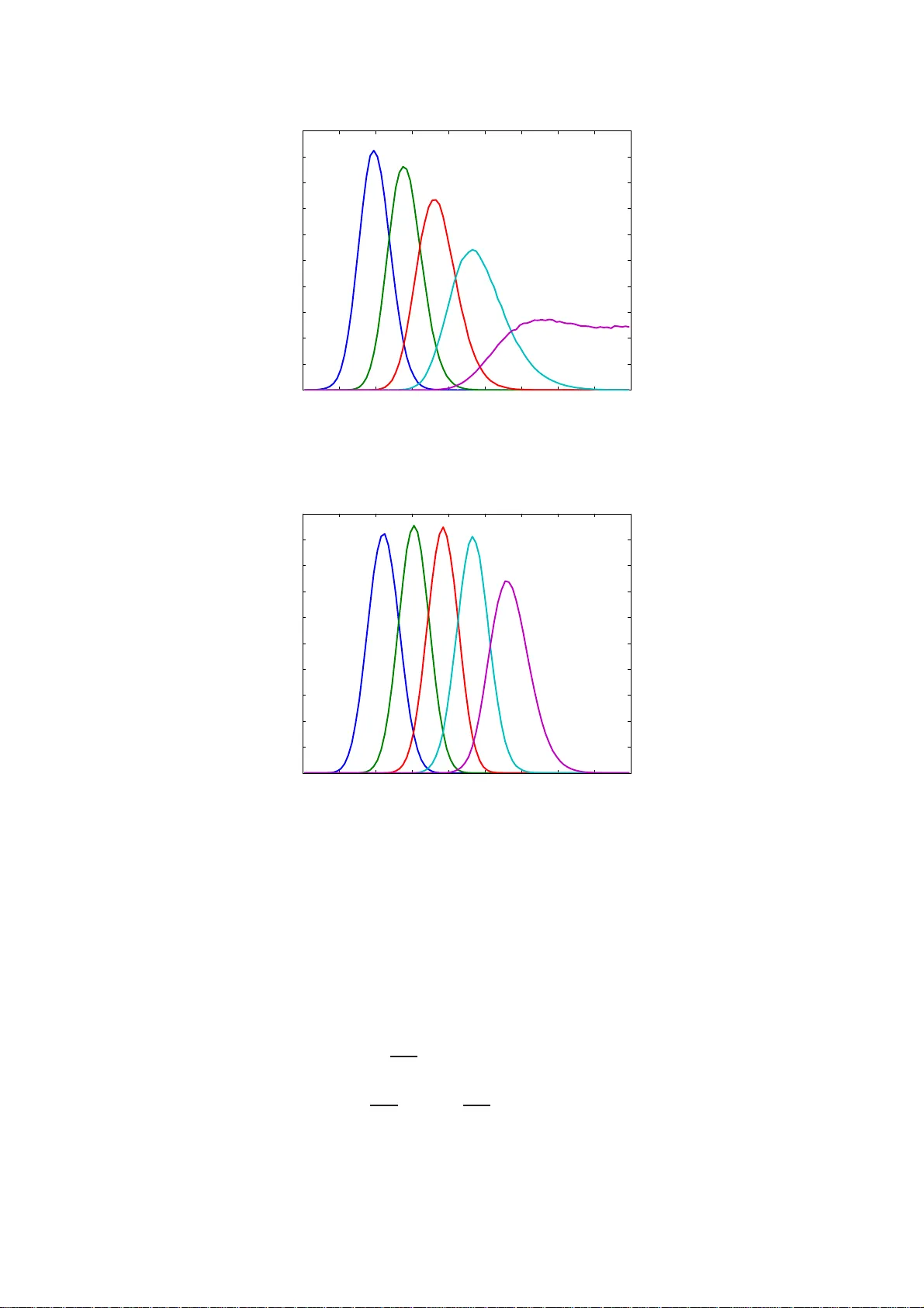
1 Minimum mean square distance estimation of a subspace Olivier Besson (1) , Nicolas Do bigeon (2) and Jean-Yves T ourneret (2) (1) Univ ersity of T oulous e, ISAE, Dep artment Electronics Optronics Sign al, T o ulouse, Fran ce (2) Univ ersity of T oulous e, IRIT/INP-ENSEEIHT/T ´ eSA, T oulous e, France olivier.bess on@isae.fr, { Nicolas.D obigeon,Jean-Yves.Tourneret } @enseeiht.fr Abstract W e con sider the problem of subsp ace estimation in a Bayesian setting. Sin ce we are op erating in the Grassman n manifold, the usual appro ach which consists of minimizin g the mean square erro r (MSE) betwee n the true sub space U and its estimate ˆ U may n ot be adequa te as the MSE is no t the natural metric in the Grassmann manifold. As an alternati ve, we p ropo se to carry out subspace estimation by minimizing the mean square distance (MSD) between U and its estimate, where the considered distance is a natura l metric in the Gr assmann manifold , viz. the distance be tween th e projection matrices. W e show that the resulting estimator is no longer the posterior mean of U but entails co mputing the principal eige n vectors of the p osterior mea n of U U T . De riv ation of th e MMSD estimator is car ried out in a f ew illustra ti ve examples includ ing a linear Gaussian mo del for th e d ata an d a Bingham or von Mises Fisher prior distribution for U . In all scenarios, posterior distributions a re deriv ed and the MMSD e stimator is obtained eithe r an alytically or implemented via a Markov chain Monte Carlo simulation method . Th e method is shown to provide accurate estimates ev en when the numb er o f samples is lower than the d imension of U . An ap plication to hyper spectral imagery is finally in vestigated. 2 I . P RO B L E M S TA T E M E N T In many signa l proce ssing ap plications, the signals of interest do not span the entire observation space an d a relev ant and frequ ently used as sumption is tha t they ev olve in a low-dimensional subspa ce [1]. Subspace modeling is a ccurate when the s ignals consist of a linea r combination of p mo des in a N -dimensional spac e, an d constitute a good approx imation for examp le wh en the signal covariance matrix is clos e to rank-de ficient. As a con seque nce, s ubspa ce estimation plays a central role in recovering these signals with maximum accuracy . An ubiquitous solution to this problem is to resort to the s ingular v alue d ecompos ition (SVD) of the d ata matrix. Th e SVD eme r ges naturally as the maximum li kelihood estimator in the classical mo del Y = U S + N , where Y s tands for the N × K observation matrix, U is the (deterministic) N × p matrix, with p < N , whos e co lumns span the p -dimensional su bspace of interest, S is the p × K ( deterministic) waveform matrix and N is the additiv e noise . The p principal left singu lar vectors of Y provide very accurate estimates of a ba sis for the range space R ( U ) of U , and h av e be en us ed successfully , e.g ., in estimating the frequencies of damp ed exp onentials or the directions of a rri val of multiple plane waves, see [2], [3] among othe rs. Howe ver , the SVD can incur some performanc e loss in two main c ases , namely when the sign al-to- noise ratio (SNR) is very low and thereof the p robability o f a s ubspa ce swap or subs pace leaka ge is h igh [4]–[7]. A secon d case occurs whe n the number of samp les K is lo wer tha n the subs pace dimension p : indeed, Y is a t mos t of rank K and information is lack ing about how to complement R ( Y ) in order to es timate R ( U ) . Under such circumstanc es, a Baye sian approach might b e helpful as it enab les one to as sist estimation by providing s ome statistical information a bout U . W e in vestigate s uch a n ap proach h erein and assign to the unkn own matrix U an approp riate p rior distrib ution, taking into accoun t the spec ific structure of U . T he p aper is organized as follo ws. In section II, we propos e an approa ch bas ed on minimizing a natural distanc e on the Grassmann ma nifold, wh ich yields a new estimator of U . The theory is illustrated in section III wh ere the new estimator is de ri ved for some s pecific examp les. In section IV its performance is asses sed through numerical simulations, and compared with con ventional approach es. Section V stud ies a n application to the an alysis of interactions betwee n p ure materials contained in hype rspectral images. I I . M I N I M U M M E A N S Q U A R E D I S TA N C E E S T I M A T I O N In this section, we intr oduce an alternati ve to the con ventional minimum mean square error (M MSE) estimator , in the cas e where a s ubspac e is to b e es timated. Let us con sider that we wis h to estimate the range spac e of U from the joint distribution p ( Y , U ) where Y stands for the av a ilable data matrix. Usua lly , one is not interes ted in U per se but rather in its range spa ce R ( U ) , and thus we are op erating in the G rassmann manifold G N ,p , i.e., the se t o f p -dimen sional sub space s in R N [8]. 3 It is thus na tural to wonder whether the MMSE e stimator (which is the chief sy stematic approac h in Bayes ian estimation [9]) is s uitable in G N ,p . The MMSE estimator ˆ θ of a vector θ minimizes the av erage Euclidean d istance between ˆ θ and θ , i.e., E     ˆ θ − θ    2 2  . Despite the fact that this distance is natural in an Euclidean space, it may not be the more natural metric in G N ,p . In fact, the natural distance be tween tw o subspace s R ( U 1 ) and R ( U 2 ) is given by  P p k =1 θ 2 k  1 / 2 [8] where θ k are the principal angles betwe en these subsp aces, wh ich c an be obtained by SVD of U T 2 U 1 where U 1 and U 2 denote orthonormal base s for the se s ubspa ces [10]. The SVD of U T 2 U 1 is d efined a s U T 2 U 1 = X diag ( cos θ 1 , · · · , cos θ p ) Z T , where X and Z are two p × p unitary matrices. The refore, it seems more adequa te, ra ther than minimizing    ˆ U − U    2 F as the MMSE estimator does, to minimize the na tural d istance b etween the subs paces spann ed by ˆ U and U . Althoug h this is the most intuiti vely appealing method, it faces the drawback that the cosines of the angles and not the angles themselves emerge naturally from the S VD. Therefore, we cons ider minimizing the s um of the squared sine of the an gles betwe en ˆ U an d U , since for s mall θ k , sin θ k ≃ θ k . As ar gued in [8], [10], this cost function is natural in the Grassmann manifold since it corres ponds to the Frobenius norm of the dif ferenc e between the projection matrices on the two sub space s, v iz P p k =1 sin 2 θ k =    ˆ U ˆ U T − U U T    2 F , d 2  ˆ U , U  . It sh ould be mentioned that our approac h follows along the sa me p rinciples a s in [11] where a Baye sian framewor k is prop osed for subs pace estimation, and w here the author conside rs minimizing d  ˆ U , U  . Hence the the ory presented in this se ction is similar to tha t o f [11], with s ome exceptions. Indeed the pa rameterization of the problem in [11] dif fers from o urs and the application of the theory is a lso very d if ferent, s ee the next se ction. Gi ven that d 2  ˆ U , U  = 2  p − T r n ˆ U T U U T ˆ U o , we defin e the minimum mea n-square distance (MMSD) e stimator of U as ˆ U mmsd = arg max ˆ U E n T r n ˆ U T U U T ˆ U oo . (1) Since E n T r n ˆ U T U U T ˆ U oo = Z  Z T r n ˆ U T U U T ˆ U o p ( U | Y ) d U  p ( Y ) d Y (2) it follows that ˆ U mmsd = arg max ˆ U Z T r n ˆ U T U U T ˆ U o p ( U | Y ) d U = arg max ˆ U T r  ˆ U T  Z U U T p ( U | Y ) d U  ˆ U  . (3) Therefore, the MMSD estimate of the subspa ce s panned by U is giv en by the p lar g est eigen vectors of the matrix R U U T p ( U | Y ) d U , which w e denote as ˆ U mmsd = P p  Z U U T p ( U | Y ) d U  . (4) 4 In other words, MMSD estimation amou nts to find the best rank- p approximation to the posterior mean of the projection matrix U U T on R ( U ) . For notationa l con venien ce, let us deno te M ( Y ) = R U U T p ( U | Y ) d U . Excep t for a few c ases where this matrix can be deri ved in c losed-form (an example is given in the next sec tion), there usually do es not exist any an alytical expression for M ( Y ) . In such situation, an efficient way to approximate the ma trix M ( Y ) is to use a Markov chain Monte Carlo s imulation method who se goal i s to generate random matrices U drawn from the posterior distrib ution p ( U | Y ) , and to approximate the integral in (4) by a finite sum. Th is asp ect will be further elabora ted in the next sec tion. Let M ( Y ) = U M ( Y ) L M ( Y ) U T M ( Y ) den ote the eigen value dec omposition of M ( Y ) with L M ( Y ) = diag ( ℓ 1 ( Y ) , ℓ 2 ( Y ) , · · · , ℓ N ( Y )) and ℓ 1 ( Y ) ≥ ℓ 2 ( Y ) ≥ · · · ≥ ℓ N ( Y ) . The n the av erage distan ce between ˆ U mmsd and U is given by E n d 2  ˆ U mmsd , U o = 2 p − 2 Z  Z T r n ˆ U T mmsd U U T ˆ U mmsd o p ( U | Y ) d U  p ( Y ) d Y = 2 p − 2 Z T r n ˆ U T mmsd M ( Y ) ˆ U mmsd o p ( Y ) d Y = 2 p − 2 p X k =1 Z ℓ k ( Y ) p ( Y ) d Y . (5) The latter expression cons titutes a lower bound on E n d 2  ˆ U , U o and is referred to a s the Hilbert- Schmidt bo und in [11], [12]. As indicated in these references, a nd s imilarly to M ( Y ) , this lo wer bound may be difficult to ob tain ana lytically . The MMSD approach can be extend ed to the mixed cas e wh ere, in addition to U , a para meter vector θ which can take arbitrary values in R q needs to be estimated jointly with U . Und er s uch circumstance s, one ca n es timate U a nd θ a s  ˆ U mmsd , ˆ θ mmsd  = arg min ˆ U , ˆ θ E  − T r n ˆ U T U U T ˆ U o +  ˆ θ − θ  T  ˆ θ − θ   . (6) Doing so, the MMSD estimator o f U is still be given b y (4) while the MMSD and MMSE estimators of θ co incide. Remark 1 The MMSD a pproach differs from a n MMSE a pproach which would e ntail calcu lating the posterior mean of U , v iz R U p ( U | Y ) d U . Note that the latter may not be meaning ful, in particular when the posterior distributi on p ( U | Y ) d epends on U only throug h U U T , see next se ction for an example. In su ch a case, post-multiplication of U by a ny p × p u nitary matrix Q yields the same value of p ( U | Y ) . Therefore av eraging U over p ( U | Y ) do es not make sen se while computing (4) is relev an t. On t he other h and, if p ( U | Y ) depe nds on U directly , then compu ting the pos terior mean of U c an be in ves tigated: an example where this situation o ccurs will b e prese nted in the next section. As a final comment, obs erve that R U p ( U | Y ) d U is not nece ssarily unitary but its range s pace can be us ed to estimate R ( U ) . 5 Remark 2 W e ope n a paren thesis here regarding the framework of this paper . Although it is not directly related to this paper (we do not address optimization problems he re) it is interesting to note the rec ent growing interes t in optimization prob lems on s pecial manifolds, espec ially on the Stiefel manifold (the s et of N × p matrices U such that U T U = I ) and the Gras smann manifold, s ee the excellent tutorial p aper b y Ed elman et al. [8] a s we ll a s [13], [14], an d [15]–[17] for s ignal p rocessing applications. Th ese references show the interes t of taking into ac count the un derlying geome try of the problem, as we attempt to do he rein. I I I . I L L U S T R A T I O N E X A M P L E S In this se ction we illustrate the previous theory o n s ome examples, including the con ventiona l linear Gaussian model (cond itioned o n U ) and a mo del in volving the eigen value d ecompos ition of the data covari ance matrix. As a fi rst step , we addre ss the issue of selecting prior distributions for U and the n move on to the de ri vation of the MMSD es timator . A. Prior distributions A crucial step in a ny Ba yesian estimation sche me c onsists of selecting the prior distribution for the variables to be estimated. W e focus here on distrib utions on the Stiefel or Gras smann ma nifold, depend ing whether we conside r the ma trix U itself or its range space . There exist only a few distrib utions on the Stiefel or Grassmann manifolds, the most widely acc epted being the Bingham or von Mises Fishe r (vMF) distributi ons [18], [19], whic h are gi ven resp ectiv ely by p B ( U ) = 1 1 F 1  1 2 p, 1 2 N ; A  etr  U T AU  (7) p vMF ( U ) = 1 0 F 1  1 2 N ; 1 4 F T F  etr  F T U  (8) where etr { . } stands for the exponen tial of the trace of the matrix betwee n braces, A is an N × N symmetric matrix, F is a n N × p arbitrary matrix, and 0 F 1 ( a ; X ) , 1 F 1 ( a, b ; X ) are hype r geometric functions of matrix arguments, se e e .g. [19] for their definitions. W e will den ote thes e d istrib utions as B ( A ) an d vMF ( F ) , respec ti vely . Ob serve that the Bingha m distribution dep ends o n U U T only , a nd can thus b e viewed as a distributi on on the Grassmann manifold [18], [19] while the vMF distrib ution depend s on U and is a d istrib ution on the Stiefel manifold. In our case, in order to introduce some knowledge a bout U , we assume that it is “close ” to a gi ven subspace spanned by the columns of an orthonormal matrix ¯ U , and he nce we consider two possible p rior distributions for U , namely π B ( U ) ∝ etr n κ U T ¯ U ¯ U T U o (9) π vMF ( U ) ∝ etr  κ U T ¯ U  (10) 6 where ∝ means “proportional to”. The distributi on in (9) is proportional to the sum of the squa red cosine angle s between R ( U ) and R  ¯ U  while π vMF ( U ) is proportional to the sum of the cosine angles betwee n R ( U ) and R  ¯ U  . Note that κ is a conc entration pa rameter: the larger κ the more concen trated around ¯ U are the subsp aces U . The difference betwee n the two distributions is the follo wing. In the Bingha m distrib ution only R ( U ) and R  ¯ U  are close (at least for large v alues of κ ) since π B ( U ) is in variant to post-multiplication of U by a ny p × p unitary matrix Q . Hence U is not n ecess arily close to ¯ U . In contrast, und er the vMF prior distrib ution, U and ¯ U a re close. For illustration p urposes , Figure 1 displays the average fraction of energy of U in R  ¯ U  defined a s AFE  U , ¯ U  = E n T r n U T ¯ U ¯ U T U o /p o . (11) As can be observed from these figures, both distributi ons allow the distance betwe en U and ¯ U to be set in a rathe r flexible way . Their AF E is shown to be identical for sma ll v alues of the c oncen tration parameter but, when κ increase s, the AFE o f the vMF distri bution inc reases faster . Additionally , even 0 10 20 30 40 50 60 70 80 90 100 0.4 0.5 0.6 0.7 0.8 0.9 1 Average fraction of energy of U in R(Ubar) Concentration parameter κ Bingham von Mises Fisher Fig. 1. A verage fraction of energy of U in R  ¯ U  versus κ . N = 20 , p = 5 . if the AFE are close for small values o f κ , the d istrib utions of the a ngles betwee n R ( U ) and R  ¯ U  exhibit so me dif ferences , as shown in Figures 2 and 3 which display the p robability density functions of thes e an gles for κ = 20 . B. Linear model In order to illustrate how the previous theory can be used in prac tice, we first con sider a simple example, namely a linear Gauss ian model (conditioned on U ), i.e., we assume that the d ata follows the mo del Y = U S + N where the columns o f N are independent and iden tically distributed (i.i.d.) Gaussian vectors with z ero-mean and (known) covari ance matrix σ 2 n I . W e assume that no kn owledge 7 0 10 20 30 40 50 60 70 80 90 0 0.01 0.02 0.03 0.04 0.05 0.06 0.07 0.08 0.09 0.1 Distribution of the angles between U and Ubar − Bingham prior Degrees Fig. 2. Distribution of the angles between R ( U ) and R  ¯ U  for a Bingha m distribution. N = 20 , p = 5 and κ = 20 . 0 10 20 30 40 50 60 70 80 90 0 0.01 0.02 0.03 0.04 0.05 0.06 0.07 0.08 0.09 0.1 Distribution of the angles between U and Ubar − vMF prior Degrees Fig. 3. Distribution of the angles between R ( U ) and R  ¯ U  for a von Mises Fisher distribution. N = 20 , p = 5 and κ = 20 . about S is available and hence its prior distrib ution is set to π ( S ) ∝ 1 . The refore, co nditioned on U we have p ( Y | U ) = Z p ( Y | U , S ) π ( S ) d S ∝ Z etr  − 1 2 σ 2 n ( Y − U S ) T ( Y − U S )  d S ∝ etr  − 1 2 σ 2 n Y T Y + 1 2 σ 2 n Y T U U T Y  . (12) 8 When U follows the Bingh am prior distribution, the posterior dis trib ution of U , c onditioned on Y is g i ven by p ( U | Y ) ∝ etr  U T  κ ¯ U ¯ U T + 1 2 σ 2 n Y Y T  U  (13) which is rec ognized as a Bingham distrib ution with parameter matrix κ ¯ U ¯ U T + 1 2 σ 2 n Y Y T , i.e., U | Y ∼ B  κ ¯ U ¯ U T + 1 2 σ 2 n Y Y T  . For such a Bingham d istrib ution, it turns out t hat the eigen vectors of R U U T p ( U | Y ) d U coincide with tho se of κ ¯ U ¯ U T + 1 2 σ 2 n Y Y T , with the same ordering o f their eigen values, s ee Appendix A for a proof. Therefore t he MMSD estimator is obtained in close d-f orm as ˆ U mmsd-LM-B = P p  κ ¯ U ¯ U T + 1 2 σ 2 n Y Y T  . (14) Therefore, the MMSD estimator ha s a very s imple form in this ca se. It co nsists of the principal subspa ce of a (we ighted) combination of the a priori p rojection matrix ¯ U ¯ U T and the information brought by the data throug h Y Y T . Ob serve that, in this particular ca se of a Bingha m pos terior , the MMSD e stimator co incides with the ma ximum a pos teriori (MAP) es timator . Let us n ow consider the ca se where the prior distribution of U is vMF , and contrast it with the previous example. Using (12) along w ith along with (10), it follo ws that the pos terior distribution now writes p ( U | Y ) ∝ etr  κ U T ¯ U + 1 2 σ 2 n U T Y Y T U  (15) which is referred to as the Bingham-von-Mises-Fisher (BMF) distrib ution with parameter matrices Y Y T , 1 2 σ 2 n I a nd κ ¯ U respectively 1 . Although this dis trib ution is kno wn [19], to our k nowledge, there does no t exist any ana lytic expression for the integral in (4) whe n U | Y has the BMF d istrib ution (15). Therefore, the MMSD estimator can not be computed in closed-form. In order to remedy this problem, a Markov chain Mon te Carlo simulation method can be a dvocated [20], [21] to ge nerate a lar ge number of matrices U ( n ) drawn from (15), and to approximate (4) as ˆ U mmsd-LM-vMF ≃ P p ( 1 N r N bi + N r X n = N bi +1 U ( n ) U ( n ) H ) . (16) In (16), N bi is the number of burn-in samples and N r is the number of sa mples used to ap proximate the estimator . An ef ficient Gibb s sampling scheme to generate random un itary matrices drawn from a BMF ( A , B , C ) distrib ution with arbitrary full-rank matrix A was p roposed in [22]. It amou nts to sampling s ucces siv ely each column of U by ge nerating a random unit no rm vector drawn from a (vector) BMF distribution. In our case, A = Y Y T whose rank is min( K, N ) an d hen ce A is rank-deficien t whenever K < N , a case of mos t interest to us. Note also that to generate ma trices U 1 The matri x X is said to have a BMF ( A , B , C ) distribution -where A i s an N × N symmetric matrix, B is a p × p diagonal matri x and C is an N × p matrix- if p ( X ) ∝ etr  C T X + B X T AX  . 9 drawn from the Bingh am distribution in (9), we need to c onsider A = ¯ U ¯ U T which has rank p < N . Therefore, the scheme of [22] n eeds to be adapted in order to gen erate r andom matrices drawn fr om (15). In Appe ndix B, we re view the me thod of [22] and sh ow ho w it can b e modified to handle the case of a rank-defic ient matrix A . Remark 3 Interestingly enough, the above es timator in (16) is the so-called indu ced arithmetic me an (IAM) [23] of the se t o f u nitary matrices U ( n ) , n = N bi + 1 , · · · , N bi + N r . It dif fers from the Karcher mean of the set U ( n ) , n = N bi + 1 , · · · , N bi + N r , which truly minimizes the s um o f the distan ces to all U ( n ) . Howev er , the Karcher mean may not exist and requires iterativ e s chemes to be computed [24] while the IAM is straightforward to comp ute. Remark 4 In the pa rticular case wh ere U has a Bingh am prior distribution, the MAP estimator of U a nd its MMSD estimator are equ al. This is no long er true when U has a vMF prior distrib ution, and hence a BMF posterior distribution. Th e mode of the latter is not known in closed-form either . Howe ver , it can be ap proximated b y selecting, a mong the matrices ge nerated by the Gibbs sampler , the matrix which results in the lar gest value of the posterior distributi on. C. Covariance matrix mode l W e now consider a more co mplicated case where Y , conditioned on U and Λ , is Ga ussian distrib uted with ze ro-mean a nd covariance matrix R = E  Y Y T  = U Λ U T + σ 2 n I (17) where U is an orthonormal ba sis for the signal sub space , Λ is the diagonal matrix of the eigen values and σ 2 n stands for the white noise power which is assumed to be known here. As it will be more con venient and mo re intuiti vely appealing, we re-pa rametrize the covariance matrix as follo ws. The in verse o f R can be written as R − 1 = U h  Λ + σ 2 n I  − 1 − σ − 2 n I i U T + σ − 2 n I = σ − 2 n I − σ − 2 n U Λ  Λ + σ 2 n I  − 1 U T , ν I − ν U ( I − Γ ) U T (18) where ν , σ − 2 n , Γ , d iag ( γ ) with γ = h γ 1 γ 2 · · · γ p i T and 0 < γ k , σ 2 n σ 2 n + λ k < 1 . (19) The idea is to parame trize the problem in terms of U and Γ rather than U and Λ . The interest of this transformation is twofold. First, it enables one to express all eigen values with respect to t he white noise lev el. Ind eed, one ha s R = ν − 1 U ⊥ U T ⊥ + ν − 1 U Γ − 1 U T where U ⊥ is an o rthonormal basis for R ( U ) ⊥ 10 and hen ce the γ k s are rep resentative of the scaling between the “sign al” e igen values and the noise eigen values. In fact, they carry information about the signal-to-noise ratio since γ k =  1 + λ k σ 2  − 1 and λ k σ 2 represents the SNR of the k -th signal compone nt. Seco nd, this new parametrization will f acilitate deriv ation of the conditional distrib utions required for the Gibbs sa mpler . Since Y conditioned o n U and γ is Gau ssian, it follows that p ( Y | U , γ ) = (2 π ) − N K/ 2 | R | − K/ 2 etr  − 1 2 Y T R − 1 Y  . (20) From R − 1 = ν U ⊥ U T ⊥ + ν U Γ U T , it en sues that   R − 1   = ν N | Γ | and henc e p ( Y | U , γ ) ∝ | Γ | K/ 2 etr  − 1 2 Y T  ν I − ν U ( I − Γ ) U T  Y  . (21) Let u s no w consider the p rior d istrib utions for U an d γ . W e will cons ider either a Bingham or vMF distrib ution for U . As for γ , we as sume tha t γ k are a priori independ ent random v ariables un iformly distrib uted in the interval [ γ − , γ + ] , i.e. , π ( γ ) = p Y k =1 ( γ + − γ − ) − 1 I [ γ − ,γ + ] ( γ k ) . (22) The value of γ + [respectiv ely γ − ] c an b e s et to 1 [respec ti vely 0 ] if a non-informati ve prior is desired. Otherwise, if some inf ormation is a vailable ab out the SNR, γ − and γ + can be chose n so as to reflect this knowledge since γ k = (1 + S N R k ) − 1 : γ + [resp. γ − ] rules the lo west [resp. highest] value of the SNR, say S N R − [resp. S N R + ]. W ith the Bingham assumption for π ( U ) , the joint pos terior distribution of U an d γ is p ( U , γ | Y ) ∝ p ( Y | U , γ ) π ( U ) π ( γ ) ∝ | Γ | K/ 2 p Y k =1 I [ γ − ,γ + ] ( γ k ) ! × etr n κ U T ¯ U ¯ U T U + ν 2 Y T U ( I − Γ ) U T Y o . (23) In orde r to come up with the posterior distrib ution of U only , we nee d to ma r ginalize (23) with respect to γ . Le t Z = Y T U = h z 1 z 2 · · · z p i . T hen, from (23) one ha s p ( U | Y ) = Z p ( U , γ | Y ) d γ ∝ etr n κ U T ¯ U ¯ U T U + ν 2 U T Y Y T U o × p Y k =1 Z γ + γ − γ K/ 2 k exp n − ν 2 γ k k z k k 2 o dγ k ∝ etr n κ U T ¯ U ¯ U T U + ν 2 U T Y Y T U o × p Y k =1 k z k k − 2(1+ K/ 2)  γ  ν 2 γ + k z k k 2 , 1 + K 2  − γ  ν 2 γ − k z k k 2 , 1 + K 2  (24) 11 where γ ( x, a ) = R x 0 t a − 1 e − t dt is the incomplete Gamma function. Unfortunately , the above distribu- tion does not belong to any known family and it is thu s problematic to generate s amples d rawn from it. Instead , in order to sample acco rding to (23), we propose to use a Gibbs sampler drawing sample s according to p ( U | Y , γ ) a nd p ( γ k | Y , U ) for k = 1 , · · · , p . F rom (23), the co nditional distribution of U is p ( U | Y , γ ) ∝ etr n κ U T ¯ U ¯ U T U + ν 2 ( I − Γ ) U T Y Y T U o (25) which is recogn ized as a (modified) Bingham distrib ution 2 U | Y , γ ∼ ˜ B  ¯ U ¯ U T , κ I , Y Y T , ν 2 ( I − Γ )  . (26) Let u s now turn to the conditional distrib ution of γ | Y , U . From (23) one has p ( γ | Y , U ) ∝ | Γ | K/ 2 etr n − ν 2 Z Γ Z T o p Y k =1 I [ γ − ,γ + ] ( γ k ) ! ∝ p Y k =1 h γ K/ 2 k exp n − ν 2 k z k k 2 γ k o I [ γ − ,γ + ] ( γ k ) i (27) which is the product of independe nt gamma distrib utions with parameters K 2 +1 a nd ν 2 k z k k 2 , truncated in the interval [ γ − , γ + ] . W e denote this d istrib ution as γ k ∼ G t  K 2 + 1 , ν 2 k z k k 2 , γ − , γ +  . Random variables with such a distributi on can be efficiently ge nerated u sing the a ccept-reject scheme of [25]. The above conditional dis trib utions can now be used in a Gibbs s ampler , as de scribed in T a ble I. When U ha s a vMF p rior distribution, it is straightforward to show that U , conditioned on Y and γ , follo ws a BMF distrib u tion U | Y , γ ∼ BMF  Y Y T , ν 2 ( I − Γ ) , κ ¯ U  while the posterior distrib ution of γ | Y , U is s till g i ven by (27). Th erefore line 2 of the Gibbs sampler in T able I just needs to be modified in order to ha ndle this cas e. Input: initial values U (0) , γ (0) 1: for n = 1 , · · · , N bi + N r do 2: sample U ( n ) from ˜ B  κ I , ¯ U ¯ U T , ν 2  I − Γ ( n − 1)  , Y Y T  in ( 25). 3: for k = 1 , · · · , p , sample γ ( n ) k from G t  K 2 + 1 , ν 2    Y T u ( n ) k    2 , γ − , γ +  in ( 27). 4: end for Output: sequen ce of random variables U ( n ) and γ ( n ) T ABLE I G I B B S S A M P L E R 2 X ∼ ˜ B ( A 1 , B 1 , A 2 , B 2 ) ⇔ p ( X ) ∝ etr  B 1 X T A 1 X + B 2 X T A 2 X  12 I V . S I M U L A T I O N S In this section we illustrate the performance of the approach developed ab ove throug h Monte Carlo simulations. In all simulations N = 20 , p = 5 and κ = 20 . T he ma trix S is gene rated from a Gaussian distrib ution with zero-mean a nd cov ariance ma trix σ 2 s I and the signal-to-noise ratio is defined a s S N R = 10 log 10  σ 2 s /σ 2 n  . T he matrix U is generated from the Bingham d istrib ution (9) or the v MF distribution (10) a nd, for the sake of s implicity , ¯ U = h I p 0 i T . The number of burn-i n iterations in the Gibbs sampler is set to N bi = 10 an d N r = 1000 . Th e MMSD estimator (4) is compared with the MAP estimator , the MMSE e stimator , the usual SVD-based es timator and the estimator ˆ U = ¯ U that disc ards the avail able data and us e only the a priori k nowledge. The latter is referred to as “ Ubar” in the figures. The es timators are evaluated in terms of the fraction of ene rgy of ˆ U in R ( U ) , i.e., AFE  ˆ U , U  . A. Linear model W e begin with the linear model. Figures 4 to 7 in vestigate the influe nce of K and S N R onto the performance of the estimators. Figu res 4 and 5 con cern the Bingham prior while the vMF prior has been used to obtain Figures 6 and 7 . From inspection of these figures, the foll owing c onclusions can be drawn: • the MMSD e stimator p erforms better than the e stimator ˆ U = ¯ U , even at low SNR. The improvement is a ll the more p ronounce d that K is lar ge . Therefore, the MMSD e stimator makes a sound us e of the da ta to improve accuracy compared to using the prior knowledge only . • the MMSD e stimator performs better than the SVD, especially at low SNR. Moreover , and this is a d istincti ve feature of this Bayesian ap proach, it enab les one to es timate the s ubspac e even when the nu mber of snaps hots K is less than the size of the subspac e p . • for a Bingham prior , the MMSE performs very po orly sinc e the po sterior distribution of U conditioned on Y depen ds on U U T only . Hence , a veraging the matrix U itself does n ot make sense , see our remark 1. In co ntrast, whe n U has a vMF prior , the posterior depe nds on both U and U U T : in this cas e, the MMSE performs well and is close to the MMSD. Note howe ver that the vMF prior is more restrictiv e than the Bingham p rior . • the MMSD es timator also outperforms the MAP estimator . As a co nclusion, the MMSD estimator performs be tter than mos t other es timators in the large majority of c ases. B. Covarianc e matrix mod el W e now condu ct simulations with the c ov ariance matrix mod el. The simulation p arameters a re essen tially the same as in the p revious sec tion, except for the SNR. More precise ly , t he random 13 variables γ k are drawn from the uniform distrib ution in (22) wh ere γ − and γ + are selected such tha t S N R − = 5 dB and S N R + = 10 dB. T he res ults are s hown in Fig. 8 for the Bingham prior and F ig. 9 for the vMF prior . They co rroborate the p revious observations made on the linear model, viz that the MMSD es timator off ers the best performanc e over all method s. V . A P P L I C A T I O N T O H Y P E R S P E C T R A L I M AG E RY In this se ction, we show ho w the proposed su bspace estimation procedu re can be ef ficiently used for an application to multi-band imag e a nalysis. F or s everal de cades , hyperspe ctral imag ery has received considerab le a ttention because of its great interest for various purpose s: a griculture monitoring, mineral mapping, military concerns, etc. One of the crucial issue when analyzing suc h image is the spectral unmixing which a ims to decompose an o bserved pixel y ℓ into a collection of R = p + 1 reference signa tures, m 1 , . . . , m R (called end members ) and to retrie ve the res pectiv e proportions of these sign atures (or abundances ) a 1 ,ℓ , . . . , a R,ℓ in this p ixel [26]. T o d escribe the phys ical process that links the end members and their a bundances to the meas urements, the most widely admitted mixing model is linear y ℓ = R X r =1 a r,ℓ m r (28) where y ℓ ∈ R N is the pixel sp ectrum mea sured in N spec tral bands, m r ∈ R N ( r = 1 , . . . , R ) are the R endmembe r s pectra and a r,ℓ ( r = 1 , . . . , R ) are their correspond ing abundan ces. Du e to obvious physica l considerations , the abundanc es obey tw o kinds of cons traints. Since they represen t proportions, they must satisfy the following po siti vity an d ad diti vity co nstraints      a r,ℓ ≥ 0 , r = 1 , . . . , R, P R r =1 a r,ℓ = 1 . (29) Let n ow c onsider L pixels y 1 , . . . , y L of an hyperspe ctral image induce d by the linear mixing model (LMM) in (28) with the ab undanc e constraints (29). It is clear that the dataset formed by these L pixels lies in a lo wer-dimensional subsp ace U ⊂ R p . More prec isely , in this subs pace U , the dataset belongs to a simplex whos e vertices are the endmembers m 1 , . . . , m R to be rec overed. Most o f the unmixing strategies developed in the h yperspe ctral imagery lit erature are base d on this und erlying geometrical formulation of the LMM. Indeed, the estimation of the en dmembers is generally condu cted in the lower -dimension al s pace U , previously ide ntified by a standard dimension reduction techniqu e such as the principal co mponent analysis (PCA) [26]. Howev er , it is we ll known that the mo del linearity is a simplifying assumption and does no t hold anymore in sev eral contexts, circumventing the s tandard unmixing algorithms. Spe cifically , non-linearities are kn own to occu r for scene s includ ing mixtures of minerals o r vegetation. As a cons equen ce, ev a luating the suitability of the LMM assu mption for a 14 giv en hyperspe ctral image is a cap ital ques tion tha t can be c on veniently ad dressed by the approa ch introduced above. A. Synthe tic data First, we in ves tigate the es timation of t he subsp ace U when the image pixels a re non-linear functions of the ab undanc es. For this purpose, a 50 × 50 synthetic hypersp ectral image is generated following a recently introduce d non-linear model referred to as ge neralized bilinear model (GBM). As indicated in [27], the GBM is notably well a dapted to des cribe non-linearities due to multi path ef fec ts. It ass umes that the ob served pixel spectrum y ℓ can be written y ℓ = R X r =1 a r,ℓ m r + R − 1 X i =1 R X j = i +1 γ i,j,ℓ a i,ℓ a j,ℓ m i ⊙ m j (30) where ⊙ stands for the Had amard (t ermwise) product and the abundances a r,ℓ ( r = 1 , . . . , R ) satisfy the constraints in (29). In ( 30), the parameters γ i,j,ℓ (which belong t o [0 , 1] ) characterize the impo rtance of non-linear interactions between the end members m i and m j in the ℓ -th pix el. In particular , when γ i,j,ℓ = 0 ( ∀ i, j ), the GBM reduce s to the stand ard LMM (28). Moreover , when γ i,j,ℓ = 1 ( ∀ i, j ), the GBM leads to the non-linear model int roduced by F an et al. in [28]. In this simulation, the synthetic image has be en generated using the GBM with R = 3 endmemb er signatures extracted from a s pectral library . The co rresponding abundances ha ve been uniforml y d rawn in the set defined by the c onstraints (29). W e have assumed tha t there is no interaction between endmemb ers m 1 and m 3 , and between endmembe rs m 2 and m 3 resulting in γ 1 , 3 ,ℓ = γ 2 , 3 ,ℓ = 0 , ∀ ℓ . Moreover , the interactions betwee n endmembe rs m 1 and m 2 are defined by the ma p of coefficients γ 1 , 2 ,ℓ displayed in Fig. 10 (top, left panel) where a black (resp. white) pixel represents the lowest (res p. highest) degree of non-linearity . As can be se en in this figure, 75% of the pixels (located in the bottom and upper right squares of the image) are mixed ac cording to the LMM res ulting in γ 1 , 2 ,ℓ = 0 . The 25% remaining image pixels (located in the uppe r left square of the image) are mixed ac cording to the GBM with nonlinearity coefficients γ 1 , 2 ,ℓ radially increas ing from 0 to 1 ( γ 1 , 2 ,ℓ = 0 in the imag e ce nter and γ 1 , 2 ,ℓ = 1 in the upper left c orner o f the image). No te that this image contains a majorit y of pixels that are mixed linearly and belong to a common subsp ace of R 2 . Con versely , the non-linearly mixed p ixels do not belong to this subs pace 3 . W e propose here to estimate the local su bspac e U ℓ where a gi ven imag e pixel y ℓ and its nearest spe ctral n eighbors V ( K − 1) ℓ li ve ( V ( K − 1) ℓ denotes the se t of the ( K − 1 )-nearest neighbors of y ℓ ). Assuming as a first approximation that all the image pixels are linearly mixed, all the se pixels are approximately c ontained in a common 2 - dimensiona l subspace ¯ U that can be determined by 3 Assuming there i s a majority of image pixels that are mixed linearly is a reasonable assumption for most hyperspectral images. 15 performing a P CA of y 1 , . . . , y L (see [29] for more d etails). The co rresponding principal vectors spanning ¯ U are gathered in a matrix ¯ U . This matrix ¯ U is use d as a prior i knowledge regarding the 2 -dimensional subspa ce co ntaining n y ℓ , V ( K − 1) ℓ o ℓ =1 ,...,L . Howe ver , t his crude estimation can be refined by the Bayesian estimation strategy de veloped in the p revious se ctions. More precise ly , for each pixel y ℓ , we compute the MMSD es timator of the N × p matrix U ℓ , whose columns are su pposed to spa n the s ubspac e U ℓ containing y ℓ and its K − 1 -nearest neighbors V ( K − 1) ℓ . T he Bayesian estimator ˆ U ℓ is compu ted from its c losed-form expression (14), i.e ., using the Bingha m prior whe re ¯ U has bee n introduc ed above. Then, for e ach pixel, we e valuate the d istance between the two projection matrices ˆ U ℓ ˆ U T ℓ and ¯ U ¯ U T onto the s ubspa ces ˆ U ℓ = R  ˆ U ℓ  and ¯ U = R  ¯ U  , respectively . As stated in S ection II, the n atural distance between the se two projection matrices is giv en by d 2  ˆ U ℓ , ¯ U  = 2  p − T r n ˆ U T ℓ ¯ U ¯ U T ˆ U ℓ o . The resulting d istance maps are depicted in Fig. 10 (bottom panels) for 2 non-zero v alues of η , 2 σ 2 n κ (as it can be noticed in (14), this hyperparame ter η balan ces the qua ntity of a pr iori knowledge ¯ U included in the estimation with respect to the information brought by the data). For co mparison p urpose, the subsp ace ˆ U ℓ has been also estimated by a crud e SVD of n y ℓ , V ( K − 1) ℓ o (top right p anel). In this case, ˆ U ℓ simply redu ces to the asso ciated principal singular vectors and can be conside red as the MMSD estimator of U ℓ obtained for η = 0 . These fig ures show that, for the 75% of the pixels generated using the LMM (bottom and right parts of the image ), the sub space ¯ U estimated by a n SVD of the wh ole datase t y 1 , . . . , y L is very close to the hyperplanes ˆ U ℓ locally estimated from n y ℓ , V ( K − 1) ℓ o through the propo sed approac h (for any value of η ). Regarding the remaining 25% pixels res ulting from the GBM (top left p art of the image), the follo wing co mments can be made. When a crude S VD of n y ℓ , V ( K − 1) ℓ o is con ducted, i.e., when n o prior knowledge is taken into accou nt to c ompute the MMSD ( η = 0 , top right panel), the distance between the locally estimated sub space ˆ U ℓ and the a priori assumed hyperplane ¯ U does not reflect the no n-linearities co ntained in the image. Con versely , wh en this crude SVD is regularized by incorporating prior knowledge with η = 0 . 5 a nd η = 50 (bo ttom left and right panels, respectively), leading to the MMSD es timator , the lar ger the degree of non-linearity , the lar ger the distance b etween ¯ U and ˆ U ℓ . T o summa rize, ev aluating the distance between the MMSD estimator ˆ U ℓ and the a priori giv en matrix ¯ U allows the degree of no n-linearity to be quantified. This interes ting property is exploited on a real hypersp ectral image in the following se ction. B. Real data The rea l h yperspec tral imag e co nsidered in this s ection has bee n ac quired in 1997 over Moffett Field, CA, by the N ASA spe ctro-imager A VIRIS. This image, d epicted with c omposite true colors in Fig. 11 (top, left panel), has bee n minutely s tudied in [29] assu ming a linear mixing mode l. T he 16 scene c onsists of a large pa rt of a lake (blac k pixels, top) and a c oastal a rea (bottom) compose d of s oil (brown pixels) and vegetation (green pixels), lea ding to R = 3 endmembers who se spe ctra and abundance map s can be fou nd in [29]. A simple es timation of a lower -dimensional spa ce ¯ U where the pixels li ve can be conducted through a direct SVD of the w hole datase t, providing the a priori matrix ¯ U . As in the previous se ction, this crude estimation can be refined by compu ting locally the MMSD estimators ˆ U ℓ spanning the subsp aces ˆ U ℓ (bottom panels). These estimators hav e been also computed with η = 0 , correspon ding to an SVD of n y ℓ , V ( K − 1) ℓ o (top, right figure). The distances between ¯ U a nd ˆ U ℓ have b een reported in the maps o f Fig. 11. Again, for η = 0 (top, right panel), a simple loc al SVD is unable to loca te possible non-linearities in the s cene. Howe ver , for two 4 non-zero values η = 0 . 5 and η = 50 (bottom left a nd right pan els, resp ectiv ely), the distances between the a p riori recovered subspa ce ¯ U and the MMSD-bas ed sub space ˆ U ℓ clearly indicate that some no n-linear effects occ ur in specific pa rts o f the image, espec ially in the lake s hore. Note that the non-linearities identified by the propose d algorithm are very similar to the o nes highlighted in [27] where the unmixing proced ure was condu cted by u sing the GBM de fined in (30). This s hows the accuracy of the propo sed MMSD estimator to loca lize the non-linearities occ urring in the sce ne, which is interesting for the an alysis of hyperspe ctral images. V I . C O N C L U S I O N S This pap er cons idered the problem o f es timating a sub space using s ome av ailable a p riori informa- tion. T ow ards this end , a Bay esian framework was advocated, where the subs pace U is a ssumed to be drawn from a n ap propriate prior distribution. Howe ver , since we o perate in a Grassman n manifold, the con ventional MMSE approa ch is questionab le as it amounts to minimizing a distan ce which is no t the most mea ningful on the Grassmann manifold. Conseque ntly , we revisited the MMSE approach a nd propo sed, as an alternativ e, to minimize a natural distance o n the Grassmann manifold. A ge neral framework was formulated resulting in a nov el estimator which entails co mputing the principal eigen vectors of the pos terior mean of U U T . The theory was exemplified on a few simple examples, where the MMSD es timator can either be obtained in closed-form or requires resorting to an MCMC simulation method. The n ew approach enables o ne to c ombine efficiently the prior knowledge and the data information, resu lting in a method that p erforms well at low S NR or with very s mall sample su pport. A successful ap plication to the ana lysis of non -linearities contained in hyperspe ctral images was also presen ted. 4 Additional results obtained with other v alues of η are av ailable online at http://dobigeon.perso .enseeiht.fr/app MMSD.html. 17 A P P E N D I X A T H E E I G E N V A L U E D E C O M P O S I T I O N O F R U U T p B ( U ) d U The purpose of this appe ndix is to prove the fol lowing proposition wh ich can be in vok ed to obtain the MMSD es timator whenever the posterior d istrib ution p ( U | Y ) is a Bingham d istrib ution. Proposition 1 Let U ∈ R N × p be an orthogona l matrix - U T U = I - drawn fr om a Bingh am distribution with p arameter matrix A p B ( U ) = exp {− κ B ( A ) } etr  U T AU  (31) with κ B ( A ) = ln 1 F 1  1 2 p, 1 2 N ; A  . Let A = U a Λ a U T a denote the e igen value decomp osition of A where the eigen values ar e or dered in desce nding or d er . Let us d efine M = R U U T p B ( U ) d U . Th en the eigen value d ecompos ition of M wr ites M = exp {− κ B ( A ) } U a Γ U T a with Γ = ∂ exp { κ B ( A ) } ∂ Λ a and γ 1 ≥ γ 2 ≥ · · · ≥ γ N where γ n = Γ ( n, n ) . Pr oo f: For notational con venien ce, let us work with the projection ma trix P = U U T whose distrib ution on the Grassma nn manifold is [19] p ( P ) = exp {− κ B ( A ) } etr { P A } . (32) W e have then that M = exp {− κ B ( A ) } Z P etr  P U a Λ a U T a  d P = exp {− κ B ( A ) } U a  Z U T a P U a etr  U T a P U a Λ a  d P  U T a = exp {− κ B ( A ) } U a  Z P etr { P Λ a } d P  U T a = exp {− κ B ( A ) } U a Γ U T a . Moreover Γ is diagonal since, for any orthogona l diagona l matrix D , Γ D = Z P D etr { P Λ a } d P = D  Z D T P D etr  D T P D D T Λ a D  d P  = D Z P etr { P Λ a } d P = D Γ 18 where, to obtain the third line, we made us e of the fact that D T Λ a D = Λ a . It follo ws tha t the eigen vectors of M and A coinc ide, and that the eige n values o f M are exp {− κ B ( A ) } γ n , for n = 1 , · · · , N . More over , it is known that exp {− κ B ( A ) } = exp {− κ B ( Λ a ) } and , from (32), one has exp { κ B ( Λ a ) } = Z etr { P Λ a } d P . Dif ferentiating the latter equa tion with resp ect to λ a ( k ) and den oting p n = P ( n, n ) , o ne ob tains ∂ exp { κ B ( Λ a ) } ∂ λ a ( k ) = ∂ ∂ λ a ( k ) Z exp ( N X n =1 λ a ( n ) p n ) d P = Z p k etr { P Λ a } d P = γ k . The previous equation enables one to relate the eigen values of A and thos e of M . It remains to prove that γ 1 ≥ γ 2 ≥ · · · ≥ γ N . T owards this end, we make use of a very general theorem due to Letac [30 ], which is briefly outlined below . Let P ( µ, A )( d X ) = exp { κ µ ( A ) } etr  X T A  µ ( d X ) be a probability asso ciated with a unitarily in variant measure µ on the set of N × N symmetric matrices. Consider the cas e of a diagonal ma trix A = d iag ( a 1 , a 2 , · · · , a N ) with a 1 ≥ a 2 ≥ · · · ≥ a N . Then [30] p roves that M = R X P ( µ, A )( d X ) is also diag onal, a nd moreover if M = diag ( m 1 , m 2 , · · · , m N ) then m 1 ≥ m 2 ≥ · · · ≥ m N . Use of this theo rem completes the proof o f the proposition. Remark 5 Most of the proposition could be proved, howe ver in a rather indirect way , us ing the results in [31]. In this reference , Jup p and Mardia c onsider maximum likeli hood estimation of the parameter matrix A from the observation of K inde pende nt matrices U k drawn from (31). Let ¯ P = K − 1 P K k =1 U k U T k and let its eigen value decompos ition be ¯ P = ¯ V ¯ D ¯ V T . Then the maximum likelihood estimate ˆ A of A has e igen value decomposition ˆ A = ¯ V D ¯ V T with ¯ d n = ∂ exp { κ B ( D ) } /∂ d n . Moreover , due to Barndorf f-Nielsen theorem for exponential f amilies, one has τ B ( ˆ A ) = Z P exp n κ B ( ˆ A ) o etr n P ˆ A o d P = ¯ V ¯ D ¯ V T which proves, since ˆ A = ¯ V D ¯ V T , tha t Z P exp { κ B ( D ) } etr n P ¯ V D ¯ V T o d P = ¯ V ¯ D ¯ V T . In [31] howev er , no results abo ut the ordering o f the eigenv a lues was giv en. 19 A P P E N D I X B S A M P L I N G F RO M T H E B I N G H A M - V O N M I S E S F I S H E R D I S T R I B U T I O N In this appendix, we show h ow to sample a u nitary random ma trix X ∈ R N × p from a (matrix) Bingham von Mises Fisher (BMF) dis trib ution, X ∼ BMF ( A , B , C ) . As will be explained shortly , this amo unts to sampling succe ssively each column of X , and entails generating a random unit norm vector dra wn from a (vector) BMF distributi on. W e briefly revie w how to sample the columns of X and the n explain how to samp le from a vec tor BMF distrib ution. A. The matrix BMF distribution The de nsity of X ∼ BMF ( A , B , C ) is given by p ( X | A , B , C ) ∝ etr  C T X + B X T AX  ∝ p Y k =1 exp  c T k x k + B ( k , k ) x T k Ax k  (33) where X = h x 1 x 2 · · · x p i and C = h c 1 c 2 · · · c p i . In [22] a Gibbs-sa mpling strategy was presented in order to sa mple from this distribution, in the c ase where A is full-rank. W e cons ider here a situation where A is rank-de ficient an d therefore we need to bring approp riate modifications to the scheme of [22] in order to handle the rank deficien cy of A . As e v idenced from (33 ) t he distrib ution of A is a product of vec tor BMF distrib utions, except that the columns of X are no t statistically indepe ndent since they are orthogo nal with probability one . Le t us rewrite X as X = h x 1 · · · x k − 1 Q ⊥ z x k +1 · · · x p i where z ∈ S N − p +1 =  x ∈ R N − p +1 × 1 ; x T x = 1  and Q ⊥ is a n N × N − p + 1 orthonormal ba sis for R ( X − k ) ⊥ where X − k stands for the matrix X with its k -th c olumn removed. As shown in [22] the c onditional de nsity of z giv en X − k is p ( z | X − k ) ∝ exp  c T k Q ⊥ z + B ( k , k ) z T Q T ⊥ AQ ⊥ z  ∝ exp n ˜ c T k z + z T ˜ Az o (34) where ˜ c k = Q T ⊥ c k and ˜ A = B ( k , k ) Q T ⊥ AQ ⊥ . Therefore, z | X − k follo ws a vector BMF dis trib ution z | X − k ∼ vBMF  ˜ A , ˜ c k  . A Markov c hain t hat con verges to BM F ( A , B , C ) can t hus be constructed as follows: Input: initial value X (0) 1: for k = 1 , · · · , p (random order) do 2: compute a bas is Q ⊥ for the null space o f X − k and s et z = Q T ⊥ x k . 3: compute ˜ c k = Q T ⊥ c k and ˜ A = B ( k , k ) Q T ⊥ AQ ⊥ . 4: sample z from a vBMF  ˜ A , ˜ c k  distrib ution ( see next sec tion ). 5: set x k = Q ⊥ z . 6: end for 20 B. The vector BMF distribution The core part o f the above algorithm, s ee line 4, is to draw a unit-norm random vector x distributed according to a vector Bingham-von Mises Fisher distribution. The latter distribution on the M - dimensional sph ere ha s a density with respe ct to the uniform distrib ution given by p ( x | c , A ) ∝ exp  c T x + x T Ax  , x ∈ S M . (35) In [22] a Gibbs-samp ling strategy was p resented in order to s ample from this distribution. While A was a ssumed to be full-rank in [22], we conside r here a situation wh ere A is rank-deficie nt, i.e . its eigen value dec omposition can be written as A = E Λ E T where E stand s for the orthonormal matrix of the e igen vectors an d Λ = diag ( λ 1 , λ 2 , · · · , λ r , 0 , · · · , 0) is the diagonal matrix of its eigen values. Our de ri vation foll ows along the same lines as in [22] with the appropriate modific ations due to the rank defic iency of A . Le t y = E T x ∈ S M and d = E T c . Since y 2 M = 1 − P M − 1 k =1 y 2 k , the uniform density in terms of the uncon strained coordina tes { y 1 , y 2 , · · · , y M − 1 } is prop ortional to | y M | − 1 and the density of { y 1 , y 2 , · · · , y M − 1 } is giv en by [22] p ( y | d , E ) ∝ exp  d T y + y T Λ y  | y M | − 1 , y 2 M = 1 − M − 1 X k =1 y 2 k ∝ exp ( M X k =1 d k y k + r X k =1 λ k y 2 k ) | y M | − 1 . (36) In orde r to sample from this d istrib ution, a Gibbs sampling strategy is ad vocated. T owards this end, we need to derive the conditional distrib utions of y k , giv en y − k where y − k stands for the vector y with its k -th component remov ed. Similarl y to [22], let us make the c hange o f v ariables θ k = y 2 k and let q = h y 2 1 1 − y 2 k y 2 2 1 − y 2 k · · · y 2 M 1 − y 2 k i T , so tha t  y 2 1 , y 2 2 , · · · , y 2 M  =  θ k , (1 − θ k ) q − k  . Since this ch ange of v ariables is not bijectiv e, i.e. y k ± θ 1 / 2 k , we need to intr oduce the sign s k of y k , and we let s = h s 1 s 2 · · · s M i T . Note that y 2 M = 1 − P M − 1 k =1 y 2 k , | y M | = (1 − θ k ) 1 / 2 q 1 / 2 M and q M = 1 − P M − 1 ℓ =1 ,ℓ 6 = k q ℓ . As s hown in [22], the Jacobia n of the transformation from { y 1 , y 2 , · · · , y M − 1 } to { θ , q 1 , · · · , q k − 1 , q k +1 , · · · , q M − 1 } is proportional to θ − 1 / 2 k (1 − θ k ) ( M − 2) / 2 Q M − 1 ℓ =1 ,ℓ 6 = k q − 1 / 2 ℓ , a nd therefore the joint distributi on of θ k , s k , q − k , s − k can be written a s p  θ k , s k , q − k , s − k  ∝ θ − 1 / 2 k (1 − θ k ) ( M − 3) / 2   Y ℓ 6 = k q − 1 / 2 ℓ   × exp    s k θ 1 / 2 k d k + (1 − θ k ) 1 / 2 X ℓ 6 = k d ℓ s ℓ q 1 / 2 ℓ    ×      exp n θ k λ k + (1 − θ k ) P r ℓ =1 ,ℓ 6 = k q ℓ λ ℓ o 1 ≤ k ≤ r exp { (1 − θ k ) P r ℓ =1 q ℓ λ ℓ } r + 1 ≤ k ≤ M . (37) It follows that 21 • for k ∈ [1 , r ] p  θ k , s k | q − k , s − k  ∝ θ − 1 / 2 k (1 − θ k ) ( M − 3) / 2 exp  θ k λ k + (1 − θ k ) q T − k λ − k  × exp  s k θ 1 / 2 k d k + (1 − θ k ) 1 / 2 h s − k ⊙ q 1 / 2 − k i T d − k  . (38) • for k ∈ [ r + 1 , M ] p  θ k , s k | q − k , s − k  ∝ θ − 1 / 2 k (1 − θ k ) ( M − 3) / 2 exp  (1 − θ k ) q T λ  × exp  s k θ 1 / 2 k d k + (1 − θ k ) 1 / 2 h s − k ⊙ q 1 / 2 − k i T d − k  . (39) In the previous equ ations, ⊙ stands for the elemen t-wise vector or matrix produ ct and q 1 / 2 − k is a short- hand no tation to des ignate the vector h q 1 / 2 1 · · · q 1 / 2 k − 1 q 1 / 2 k +1 · · · q 1 / 2 M i T . In order to sample from p  θ k , s k | q − k , s − k  , we first sample θ k from p  θ k | q − k , s − k  = p  θ k , s k = − 1 | q − k , s − k  + p  θ k , s k = 1 | q − k , s − k  ∝ θ − 1 / 2 k (1 − θ k ) ( M − 3) / 2 exp n a k θ k + b k (1 − θ k ) 1 / 2 o × h exp n − d k θ 1 / 2 k o + exp n − d k θ 1 / 2 k oi (40) where b k = h s − k ⊙ q 1 / 2 − k i T d − k and a k =      λ k − q T − k λ − k k ∈ [1 , r ] − q T λ k ∈ [ r + 1 , M ] . (41) Next, we s ample s k ∈ {− 1 , +1 } with proba bilities proportional to  e − d k θ 1 / 2 k , e + d k θ 1 / 2 k  . In order to sample from the distribution in (40), a n efficient rejection sa mpling sc heme was propos ed in [22], where the propo sal distribut ion is a be ta distribution with suitably c hosen parame ters. A C K N O W L E D G M E N T The authors would like to thank Prof. Kit Bigh am from the Uni versity of Mi nnes ota for insightful comments on the Bingham distribution and for pointing reference [31]. They are also indebted to Prof. G ´ erard Le tac, Un i versity o f T oulouse , for fruitf ul d iscussion s leading to the proof of Prop osition 1 gi ven in Ap pendix A. R E F E R E N C E S [1] L. L. Scharf, Statistical Signal Pr ocessing: Detection, E stimation and T ime Series Analysis . Reading, MA: Addison W esley , 1991. [2] R. Kuma resan and D. T ufts, “Estimating the parameters of expo nentially damped sinusoids and pole-zero modeling in noise, ” IEEE T rans actions Acoustics Speech Signal Pro cessing , vol. 30, no. 6, pp. 833–840 , Decemb er 1982. [3] ——, “Estimating the angles of arri val of multiple plane waves, ” IEEE T ransa ctions Aer ospace Electr onic Systems , vol. 19, no. 1, pp. 134–139 , Jan uary 1983. 22 [4] J. Thomas, L . Scharf, and D. T ufts, “The probability of a subspace swap in t he SVD, ” IEEE Transactions Signal Pr ocessing , vo l. 43, no. 3, pp. 730–736, March 1995. [5] M. Hawkes, A. Nehorai, and P . Stoica, “Performance breakdo wn of subspace-based methods: prediction and cure, ” i n Pr oceedings ICASSP , May 2001, pp. 4005–400 8. [6] B. Johnson, Y . Abramovich , and X. Mestre, “The role of subspace swap in MUSIC performance breakdo wn, ” i n Pr oceedings ICASSP , March 2008, pp. 2473 –2476. [7] R. R. Nadakuditi and F . Benaych-Geor ges, “The breakdo wn point of signal subspace estimation, ” in Pr oceedings SAM , Israel, 4-7 October 2010, pp. 177–180. [8] A. Edelman, T . Arias, and S. Smith, “The geometry of algorithms wit h orthogonality constraints, ” SIAM Journal Matrix Analysis Applications , vol. 20, no. 2, pp. 303–353, 1998. [9] S. M. Kay , Fundamentals of Statistical Signal Pr ocessing: Estimation Theory . E ngle wood Cliffs, NJ: Prentice Hall, 1993. [10] G. Golub and C. V . Loan, Matrix Computations , 3rd ed. Baltimore: John Hopkins Uni versity Press, 1996. [11] A. Sriv astava, “ A Bayesian approach to geometric subspace estimation, ” IEEE Transactions Signal Processin g , vol. 48, no. 5, pp. 1390–1400, Ma y 2000. [12] U. Grenander , M. I. Miller , and A. Sr iv astav a, “Hilbert-Schmidt lower bound s for estimators on matrix Lie groups for A TR, ” IEE E Tr ansactions P attern Analysis Machin e Intelligence , vol. 20, no. 8, pp. 790–802 , Aug ust 1998. [13] P .-A. Absil, R . Mahony , and R. S epulchre, O ptimization algorithms on matrix manifolds . Princeton, NJ: P rinceton Univ ersity Press, 2008. [14] P .-A. Absil, “Optimization on manifolds: Methods and applications, ” Uni versit ´ e Catholique L ouv ain, T ech. Rep. UCL- INMA-2009.043 , 20 09. [15] T . E . Abrudan, J. E riksson, and V . Ko ivu nen, “Steepest descent algorithms for optimization under unitary matrix constraint, ” IEEE Transac tions Signal Pr ocessing , vol. 56, no. 3, pp. 1134–114 7, March 2008. [16] ——, “Conjugate gradient algorithm for optimization under unitary matrix constraint, ” Signal Pr ocessing , vol. 89, pp. 1704–1 714, 20 09. [17] S. Fiori and T . T anaka, “ An algorithm to compute averages on matrix lie grou ps, ” IE EE Transaction s Signal Proc essing , vol. 57, no. 12, pp. 4734–4 743, Dece mber 2009. [18] K. V . Mardia and P . E . Jupp, Dir ectional Statistics . John W iley & Sons, 1999. [19] Y . Chikuse, Statistics on special manifolds . New Y ork: Springer V erlag, 2003. [20] C. P . Robert and G. Casella, Monte Carlo Statistical Methods , 2nd ed. New Y ork: Springer V erlag, 2004. [21] C. P . Robert, T he Bayesian Choice - F ro m Decision-Theor etic F oundations to Computational Implementation . New Y ork: Springer V erlag, 2007. [22] P . D. Hof f, “Simulation of the matrix Bingham -von Mises-Fisher distribution, with applications to multiv ariate and relational data, ” J ournal of Computational and Gr aphical Statistics , vol. 18, no. 2, p p. 438–456 , June 2009. [23] A. Sarlette and R. Sepulch re, “Consensu s optimization on manifolds, ” SIAM Journa l Contr ol Optimization , v ol. 48, no. 1, pp. 56–76, 2009. [24] E. Begelfor and M. W erman, “ Af fine in variance r e visited, ” in Pr oceedings IE EE C VPR06 , 2006, pp. 2087–2094. [25] Y . Chun g, “Simulation of truncated gamma variables, ” Ko r ean J . Comput. Appl. Math. , v ol. 5, no . 3, pp. 60 1–610, 1998. [26] N. Kesh av a and J. Mustard, “Spectral unmixing, ” IEEE Signal Pr ocessing Magazine , vol. 19, no. 1, pp. 44–57, January 2002. [27] A. Halimi, Y . Altmann, N. Dobigeo n, and J.-Y . T ourneret, “Nonlinear unmixing of hyperspectral images using a generalized bilinear model, ” I EEE T ransactions Geoscience Remote Sensing , 2011, to appear . 23 [28] W . Fan, B. Hu, J. Miller, and M. Li, “Comparativ e study between a ne w nonlinear model and common linear model for analysing laboratory si mulated-forest hyperspectral data, ” Internationa l J ournal Remote Sensing , v ol. 30, no. 11, pp. 2951–29 62, Jun e 2009. [29] N. Dobigeon, S. Moussaou i, M. Coulon, J.-Y . T ourneret, and A. Hero, “Joint Bayesian endmember extraction and linear unmixing for hyperspectral i magery , ” IEEE T ransactions on Signal Pro cessing , vol. 57, no. 11, pp. 4355 –4368, Nov ember 2009. [30] G. Letac, “Familles exponentielles inv ariantes sur les matrices sym ´ etriques, ” December 2010, priv at e communication. [31] P . E. Jupp and K. V . Mardia, “Maximum li kelihood estimators for the matrix Von Mises-Fi sher and B ingham distributions, ” The Annals of Statistics , vo l. 7, no. 3, pp. 599–606, M ay 1979. 24 2 4 6 8 10 12 14 16 18 0 0.1 0.2 0.3 0.4 0.5 0.6 0.7 0.8 0.9 1 Number of snapshots MMSD MMSE Ubar SVD Fig. 4. Fraction of energ y of ˆ U in R ( U ) versus K . N = 20 , p = 5 , κ = 20 and S N R = 5 dB. L inear model, Bingham prior . −6 −4 −2 0 2 4 6 8 10 0.35 0.4 0.45 0.5 0.55 0.6 0.65 0.7 0.75 0.8 0.85 Signal to Noise Ratio (dB) MMSD MMSE Ubar SVD Fig. 5. F raction of ener gy of ˆ U in R ( U ) versus S N R . N = 20 , p = 5 , κ = 20 and K = 5 . Linear model, Bingh am prior . 25 2 4 6 8 10 12 14 16 18 0 0.1 0.2 0.3 0.4 0.5 0.6 0.7 0.8 0.9 1 Number of snapshots MMSD MMSE MAP Ubar SVD Fig. 6. Fraction of energy of ˆ U in R ( U ) v ersus K . N = 20 , p = 5 , κ = 20 and S N R = 5 dB. Linear mode l, vMF prior . −6 −4 −2 0 2 4 6 8 10 0.35 0.4 0.45 0.5 0.55 0.6 0.65 0.7 0.75 0.8 Number of snapshots MMSD MMSE MAP Ubar SVD Fig. 7. Fraction of energy of ˆ U i n R ( U ) versus S N R . N = 20 , p = 5 , κ = 20 and K = 5 . Linear model, vMF prior . 26 2 4 6 8 10 12 14 16 18 0 0.1 0.2 0.3 0.4 0.5 0.6 0.7 0.8 0.9 Number of snasphots MMSD MMSE MAP Ubar SVD Fig. 8. Fraction of ener gy of ˆ U in R ( U ) versus K . N = 20 , p = 5 , κ = 20 , S N R − = 5 dB and S N R + = 10 dB. Cov ariance matrix model, Bingham prior . 2 4 6 8 10 12 14 16 18 0 0.1 0.2 0.3 0.4 0.5 0.6 0.7 0.8 0.9 Number of snasphots MMSD MMSE MAP Ubar SVD Fig. 9. Fraction of ener gy of ˆ U in R ( U ) versus K . N = 20 , p = 5 , κ = 20 , S N R − = 5 dB and S N R + = 10 dB. Cov ariance matrix model, vMF prior . 27 10 20 30 40 50 10 20 30 40 50 10 20 30 40 50 10 20 30 40 50 10 20 30 40 50 10 20 30 40 50 10 20 30 40 50 10 20 30 40 50 Fig. 10. T op, left : non-linearity coef ficients γ 1 , 2 . T op, right: distance between ¯ U and ˆ U n estimated wit h η = 0 . Bottom: distance between ¯ U and ˆ U ℓ estimated with η = 0 . 5 (left) and η = 50 (right). 10 20 30 40 50 10 20 30 40 50 10 20 30 40 50 10 20 30 40 50 10 20 30 40 50 10 20 30 40 50 10 20 30 40 50 10 20 30 40 50 Fig. 11. T op, left: The Mof fett F ield scene as composite true colors. T op, right: distance between ¯ U and ˆ U n estimated with η = 0 . Bottom: distance between ¯ U and ˆ U ℓ estimated wit h η = 0 . 5 (left) and η = 50 (right).