Three-dimensional rogue waves in non-stationary parabolic potentials

Using symmetry analysis we systematically present a higher-dimensional similarity transformation reducing the (3+1)-dimensional inhomogeneous nonlinear Schrodinger (NLS) equation with variable coefficients and parabolic potential to the (1+1)-dimensional NLS equation with constant coefficients. This transformation allows us to relate certain class of localized exact solutions of the (3+1)-dimensional case to the variety of solutions of integrable NLS equation of (1+1)-dimensional case. As an example, we illustrated our technique using two lowest order rational solutions of the NLS equation as seeding functions to obtain rogue wave-like solutions localized in three dimensions that have complicated evolution in time including interactions between two time-dependent rogue wave solutions. The obtained three-dimensional rogue wave-like solutions may raise the possibility of relative experiments and potential applications in nonlinear optics and BECs.

💡 Research Summary

The paper addresses the challenging problem of finding exact, analytically tractable solutions for a (3+1)-dimensional inhomogeneous nonlinear Schrödinger (NLS) equation whose coefficients—dispersion, nonlinearity, and external potential—are allowed to vary in time. The authors employ Lie symmetry analysis to uncover a continuous symmetry group of the governing equation and, based on this group, construct a higher‑dimensional similarity transformation that maps the original equation onto the standard integrable (1+1)-dimensional NLS with constant coefficients.

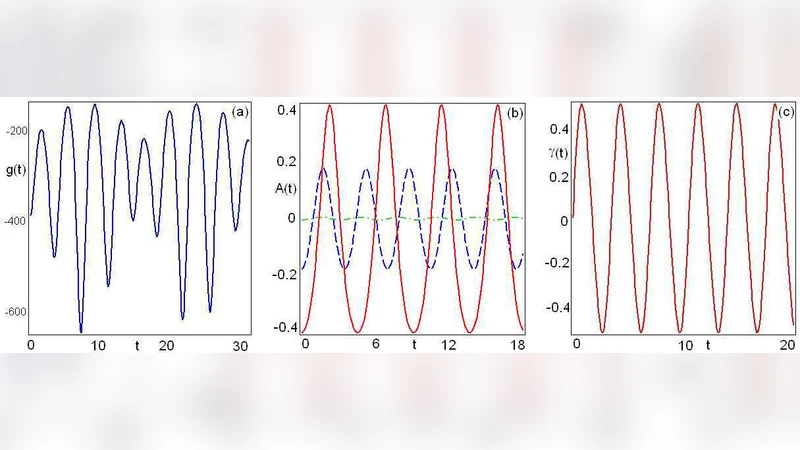
The transformation introduces a time‑dependent scaling function (a(t)), a phase function (\theta(t)), and a rotated spatial coordinate (\xi). By substituting the transformed variables into the original equation, a set of consistency conditions emerges: the dispersion must satisfy (\alpha(t)=a(t)^2), the nonlinearity must scale as (g(t)=g_0 a(t)^{-1}), and the parabolic potential strength must obey (\Omega(t) = -\ddot a(t)/a(t)). When these relations hold, the (3+1)‑dimensional problem collapses exactly to the familiar NLS
\