An Analysis of Active Learning With Uniform Feature Noise

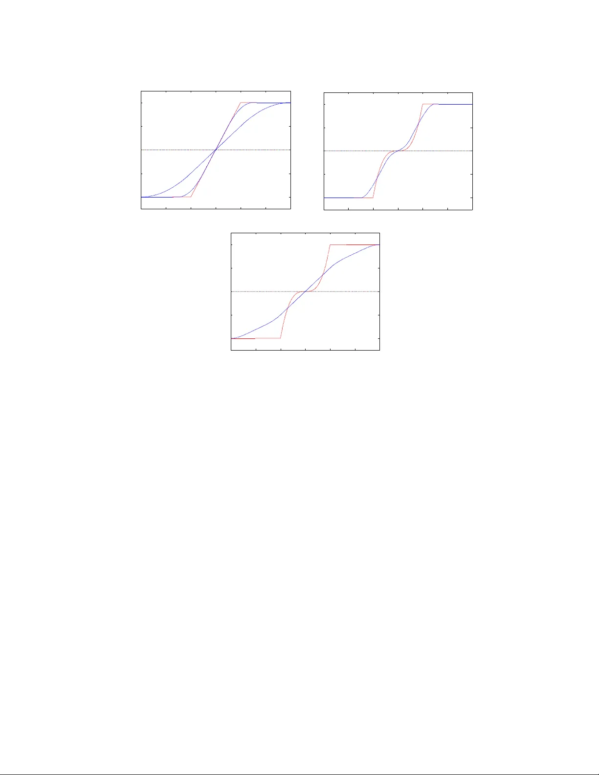
An Analysis of Activ e Learning With Uniform F eature Noise Aadit ya Ramdas 12 aramdas@cs.cmu.edu Barnab´ as P´ oczos 2 bapoczos@cs.cmu.edu Aarti Singh 2 aarti@cs.cmu.edu Larry W asserman 12 larry@stat.cmu.edu Departmen t of Statistics 1 and Machine Learning Department 2 Carnegie Mellon Univ ersity August 6, 2018 Abstract In activ e learning, the user sequen tially chooses v alues for feature X and an oracle returns the corresponding lab el Y . In this paper, we consider the effect of feature noise in active learning, which could arise either b ecause X itself is b eing measured, or it is corrupted in transmission to the oracle, or the oracle returns the lab el of a noisy v ersion of the query p oin t. In statistics, feature noise is kno wn as “errors in v ariables” and has b een studied extensiv ely in non-active settings. How ever, the effect of feature noise in active learning has not been studied b efore. W e consider the w ell-known Berkson errors-in-v ariables mo del with additiv e uniform noise of width σ . Our simple but revealing setting is that of one-dimensional binary classification setting where the goal is to learn a threshold (p oin t where the probability of a + lab el crosses half ). W e deal with regression functions that are antisymmetric in a region of size σ around the threshold and also satisfy Tsybak ov’s margin condition around the threshold. W e pro ve min- imax low er and upp er b ounds which demonstrate that when σ is smaller than the minimiax activ e/passive noiseless error derived in Castro & Now ak (2007), then noise has no effect on the rates and one achiev es the same noiseless rates. F or larger σ , the unflattening of the regression function on conv olution with uniform noise, along with its lo cal an tisymmetry around the threshold, together yield a b ehaviour where noise app e ars to b e b eneficial. Our k ey result is that activ e learning can buy significan t improv ement ov er a passive strategy ev en in the presence of feature noise. 1 In tro duction Activ e learning is a machine learning paradigm where the algorithm in teracts with a lab el- pro viding oracle in a feedbac k driven loop where past training data (features queried and cor- resp onding lab els) are used to guide the design of subsequen t queries. Typically , the oracle is 1 queried with an exact feature v alue and the oracle returns the lab el corresponding precisely to that feature v alue. How ever, in many scenarios, the feature v alue b eing queried can b e noisy and it helps to analyze what would happ en in such a setting. Suc h situations include noisy sensor measuremen ts of features, corrupted transmission of data from source to storage, or just access to a limited noisy oracle. The errors-in-v ariables mo del has been well studied in the statistical literature and their effect can b e profound. In densit y estimation, Gaussian error causes the minimax rate to b ecome logarithmic in sample size instead of polynomial, see F an (1991). F or results in passive regression, refer to F an et al. (1993); F uller (2009); Carroll et al. (2010), and for passive classification, see Loustau & Marteau (2012). Ho wev er, classification has not b een studied in the Berkson mo del introduced b elow. Also, decon volution estimators require the noise fourier transform to b e b ounded aw ay from zero, ruling out uniform noise. Finally , to the b est of our knowledge, feature noise has not b een studied for activ e learning in an y setting. The classic al err ors in variables mo del has the graphical form W ← X → Y , represen ting W = X + δ , Y = m ( X ) +  . Here, the label Y depends on the feature X but we do not observe X ; rather w e observ e the noisy feature W . The Berkson err ors in variables mo del is X = W + δ , Y = m ( X ) +  . The difference is that w e start with an observed feature W and then noise is added to determine X . Graphically , this mo del is W → X → Y . In this pap er, we fo cus on the Berkson error model since it intuitiv ely mak es more sense for activ e learning - it captures the idea that w e request a lab el for feature W , but the oracle returns the lab el for X which is a corrupted version generated from W , i.e. the noise o ccurs b etw een the lab el request and the oracle output. W e use uniform noise since it yields insightful b ehavior and also has not b een addressed in the literature. W e conjecture that qualitatively similar results hold for other symmetric error models. 1.1 Setup Threshold Classification. Let X = [ − 1 , 1], Y = { + , −} , and f : X → Y denote a classifi- cation rule. Assuming 0 / 1 loss, the risk of the classification rule f is R ( f ) = E [1 { f ( X ) 6 = Y } ] = P ( f ( X ) 6 = Y ). It is known that the Bay es optimal classifier, the b est measurable classifier that minimizes the risk f ∗ = arg min f R ( f ), has the follo wing form f ∗ ( x ) = ( + if m ( x ) ≥ 1 / 2 , − if m ( x ) < 1 / 2 , where m ( x ) = P ( Y = + | X = x ) is the unknown regression function. In what follows, we will consider the case where the f ∗ is a threshold classifier, i.e. there exists a unique t ∈ [ − 1 , 1] with m ( t ) = 1 / 2 suc h that m ( x ) < 1 / 2 if x < t , and m ( x ) > 1 / 2 if x > t . 2 Berkson Error Mo del. The mo del is: 1. User c ho oses W and requests lab el. 2. Oracle receiv es a noisy W namely X = W + U . 3. Oracle returns Y where P ( Y = + | X = x ) = m ( x ). W e tak e the noise to b e uniform: U ∼ Unif [ − σ, σ ], where the noise width σ is known for simplicit y . Sampling Strategies. In p assive sampling , assume that we are given a batch of w i ∼ Unif [ − 1 , 1] and corresp onding lab els y i sampled indep endently of { w j } j 6 = i and { y j } j 6 = i . In this case, a strat- egy S is just an estimator S n : ( W × Y ) n → [ − 1 , 1] that returns a guess b t of the threshold t on seeing { w i , y i } n i =1 . In active sampling w e are allow ed to sequentially choose w i = S i ( w 1 , . . . , w i − 1 , y 1 , . . . , y i − 1 ), where S i is a p ossibly random function of past queries and lab els, where the randomness is indep enden t of queries and lab els. In this case, a strategy A is a sequence of functions S i : ( W × Y ) i − 1 → [ − 1 , 1] returning query p oints and an estimator S n : ( W × Y ) n → [ − 1 , 1] that returns a guess b t at the end. Let S P n , S A n b e the set of all passive or activ e strategies (and estimators) with a total budget of n labels. T o av oid the issue of noise resulting in a p oint outside the domain, w e make a (Q)uerying assumption: (Q). Querying within σ of the b oundary is disallow ed. Loss Measure. Let b t = b t ( W n 1 , Y n 1 ) denote an estimator of t using n samples from a passive or activ e strategy . Our task will b e to estimate the lo cation of t , where w e measure accuracy of an estimator b t b y a loss function which is the point error | b t − t | . F unction Class. In the analysis of rates for classification (among others), it is common to use the Tsyb akov Noise/Mar gin Condition (see Tsybako v (2004)), to characterize the b ehavior of m ( x ) around the threshold t . Given constants c, C with C ≥ c , k ≥ 1, and noise level σ , let P ( c, C , k , σ ) b e the set of regression functions m ( x ) that satisfy the following conditions (T,M,B) for some threshold t : (T). | x − t | k − 1 ≥ | m ( x ) − 1 / 2 | ≥ c | x − t | k − 1 whenev er | m ( x ) − 1 / 2 | ≤  0 for some constant  0 (M). m ( t + δ ) − 1 / 2 = 1 / 2 − m ( t − δ ) for all δ ≤ σ . (B). t is at least σ a wa y from the b oundary . On adding noise U , the p oint where m ? U ( ? means conv olution) crosses half may differ from t , the p oin t where m crosses half. How ever, the antisymmetry assumption (M) and b oundary assumption (B) together imply that the tw o thresholds are the same. Getting rid of (M,B) seems substan tially difficult. When σ = 0, (Q), (M) and (B) are v acuously satisfied, and this is exactly the class of functions and strategies considered in Castro & Now ak (2007). Smaller k means that the regression function 3 is steeper, which makes it easier to estimate the threshold and classify future labels (cf. Steinw art & Sco vel (2004)). k = 1 captures a discon tinuous m ( x ) jumping at t . Minimax Risk. W e are interested in the minimax risk under the p oint error loss : R n ( P ( c, C , k , σ )) = inf S ∈S n sup P ∈P ( c,C,k,σ ) E | b t − t | (1) where S n is the set of strategies accessing n samples. F or brevity , R P n ( k , σ ) or R A n ( k , σ ) denotes risk for (P)assive/(A)ctiv e sampling stratgies S P n , S A n . Notation ≺ ,  ,  ,  ,  . W e analyse minimax p oin t error rates in different regimes of σ as a function of n (or equiv alently , for a given p oin t error, we can analyse how the sample size n dep ends on σ ) and w e write σ n for emphasis. In this pap er, f n ≺ g n means f n /g n → 0, f n  g n means c 1 g n ≤ f n ≤ c 2 g n where c 1 , c 2 are constan ts, f n  g n means f n ≺ g n or f n  g n , f n  g n means g n  f n and f n  g n means g n ≺ f n . 2 Main Result and Comparisions The main result of this paper is as follo ws. Theorem 1. Under the Berkson err or mo del, when given n lab els sample d actively or p assively with assumption (Q), and when the true underlying r e gr ession function lies in P ( c, C , k , σ n ) for known k , σ n , the minimax risk under the p oint err or loss is: 1. R P n ( P ( k , σ ))  ( n − 1 2 k − 1 if σ n ≺ n − 1 2 k − 1 σ − ( k − 3 2 ) n q 1 n otherwise 2. R A n ( P ( k , σ ))  ( n − 1 2 k − 2 if σ n ≺ n − 1 2 k − 2 σ − ( k − 2) n q 1 n otherwise When k = 1, m ( x ) jumps at the threshold, and we interpret the quantit y n − 1 2 k − 2 as b eing exp onen tially small, i.e. b eing smaller than n − p for an y p . W e also suppress logarithmic factors in n, σ n . If the domain was [ − R, R ], the corresp onding passiv e rates are obtained by substituting n b y n/R , but activ e rates remain the same upto logarithmic factors in R . Remark. In this pap er, we fo cus on learning the threshold t . This is relev ant b ecause the threshold maybe of intrinsic interest, and also of in terest for prediction if, for example, future queries could b e made with a different noise mo del or can be obtained (with some cost) noise-free. Similar results can b e deriv ed for 0/1-risk. Zero Noise. When σ = 0, the assumptions (Q,B,M) are v acuously true, and our class P ( c, C , k , 0) matc hes the class P ( c, C , k ) considered in Castro & Now ak (2007), and our rates for σ = 0 i.e. n − 1 2 k − 1 and n − 1 2 k − 2 are precisely the passive and active minimax point error rates in Castro & No wak (2007). 4 Small Noise. When the noise is small, we get what w e exp ect - the risk do es not c hange with noise as long as the noise itself is smaller than the noiseless error. In other words, as long as the noise is smaller than the noiseless error rate of n − 1 2 k − 1 for passive learning, passive learners will not really b e able to notice this tiny noise, and the minimax rate remains n − 1 2 k − 1 . Similarly , as long as the noise is smaller than the noiseless error rate of n − 1 2 k − 2 for active learning, active learners will not really b e able to notice this tiny noise, and the minimax rate remains n − 1 2 k − 1 . Also, the passive rates v ary smo othly - at the p oint when σ n  n − 1 2 k − 1 , the rates for small and large noise coincide. Similarly , at the point when σ n  n − 1 2 k − 2 , the aforementioned active rates for small and large noise coincide. Large Noise and Assumption (M). When the noise is large, we see a curious b ehaviour of the rates. When k > 2, the error rates seem to get smaller/b etter with larger noise for b oth activ e and passive learning, and furthermore the noisy rates can also b e b etter than the noiseless rate! This might seem to violate b oth the information pro cessing inequalit y , and our in tuition that more noise shouldn’t help estimation. Moreo ver, a noiseless active learner may be able to sim ulate a noisy situation b y adding noise and querying at the resulting p oint, and get b etter rates, violating low er b ounds in Castro & No wak (2007). Ho wev er, we make the following crucial but subtle observ ation. Our claimed rates are not ab out a fixed function class - due to assumption (M), the function class c hanges with σ , and in fact (M) requires the antisymmetry of the regression function to hold ov er a larger region for larger σ . This set of functions is actually getting smaller with larger σ . Ev en though the functions can b eha ve quite arbitrarily outside ( t − σ, t + σ ), this assumption (M) on a small region of size 2 σ actually helps us significantly . Giv en that there is no con tradiction to the results of Castro & Now ak (2007) or more funda- men tal information theoretic ideas, there is also an intuitiv e explanation of why assumption (M) helps when we ha ve large noise. As we will see in a later figure, con volution with noise seems to “stretc h/unflatten” the function around the threshold. Sp ecifically , for larger k > 2, the regres- sion function can b e quite flat around the threshold - conv olution with noise makes it less flat and more linear - in fact it b ehav es linearly ov er a large region of width nearly 2 σ . This is true regardless of whether assumption (M) holds - how ev er if (M) do es not hold, then the conv olved threshold, which is the p oint where the conv olv ed function crosses half, need not be the original threshold t . While dropping assumption (M) will not hurt if we only w ant to find the con volv ed threshold, but giv en that our aim is to estimate t , the problem of figuring out how m uch the threshold shifted can b e quite non-trivial. Hence, large noise ensures a b eha viour that is less flat and more linear around the threshold, and assumption (M) ensures that the threshold do esn’t shift from t . In tuitively this is why (M) and large noise help, and technically there is no contradiction b ecasue the function class is getting progressiv ely simpler b ecause of more con trolled growth around the threshold. The main takea wa y is that in all settings, active learning yields a gain ov er passive sampling. W e no w describ e the upp er and lo wer b ounds that lead to Theorem 1. The case k = 1 is handled in detail for intuition b but proofs for k > 1 are in the App endix. 5 0.2 0.3 0.4 0.5 0.6 0.7 0.8 0.3 0.4 0.5 0.6 0.7 Query Domain η (x) in red, F(w) in blue 0.2 0.3 0.4 0.5 0.6 0.7 0.8 0.3 0.4 0.5 0.6 0.7 Query Domain η (x) in red, F(w) in blue 0.2 0.3 0.4 0.5 0.6 0.7 0.8 0.3 0.4 0.5 0.6 0.7 Query Domain η (x) in red, F(w) in blue Figure 1: Regression function η ( x ) (red) b efore and F ( w ) (blue) after conv olution with noise. In all 3 figures, Tsybako v’s margin condition holds for x ∈ [0 . 4 , 0 . 6]. The top plot has a linear regression function ( k = 2), and its t wo blue curves are for σ n = 0 . 05 ( nar r ow ) , 0 . 2 ( w ide ), and they show that a linear gro wth around t = 0 . 5 remains linear. The middle and b ottom figure are for a flatter regression function with k = 4, and σ n = 0 . 05 , 0 . 2 resp ectively , plotted separately for clarity . k = 4 is harder than for k = 2 b ecause the red curve is flatter around t , making it harder to pinp oint the threshold. How ev er, as one can see in b oth plots, noise actually helps by smo othing it out and making it more linear. Ho wev er, note that the effect of assumption (M) cannot b e understated, due to which in all plots the threshold b efore and after noise cross half at the same p oin t. The effect of noise when k = 1 can b e seen in the follo wing section. 2.1 Sim ulation of Noise Conv olution 2.2 P ap er Roadmap W e devote the next tw o sections to proving the lo wer and upp er b ounds, in that order, that lead to Theorem 1. While the pro ofs will b e self-contained, we lea ve some detailed calculations to the app endix. F or easier readibility , we presen t lo wer b ounds for k = 1 first to absorb the technique and then the lo wer b ounds for k > 1. In Section 2 we will pro ve Theorem 2 (Low er Bounds) . Under the Berkson err or mo del and assumption (Q), 6 1. F or k = 1 , the p assive/active lower b ounds ar e inf S ∈S P n sup P ∈P (1 ,σ n ) E | b t − t |  ( 1 n if σ n ≺ 1 n p σ n n otherwise inf S ∈S A n sup P ∈P (1 ,σ n ) E | b t − t |  ( e − n if σ n ≺ e − n σ n √ n otherwise 2. F or k > 1 , the p assive/active lower b ounds ar e inf S ∈S P n sup P ∈P ( k,σ n ) E | b t − t |  ( n − 1 2 k − 1 if σ n ≺ n − 1 2 k − 1 σ − ( k − 3 2 ) n q 1 n otherwise inf S ∈S A n sup P ∈P ( k,σ n ) E | b t − t |  ( n − 1 2 k − 2 if σ n ≺ n − 1 2 k − 2 σ − ( k − 2) n q 1 n otherwise F ollowing that, we again present activ e and passiv e algorithms for k = 1 first to gather in tuition and then generalize them for k > 1. In Section 3 we will pro ve Theorem 3 (Upp er Bounds) . Under the Berkson err or mo del and assumption (Q), 1. F or k = 1 , a p assive algorithm (WIDEHIST) and an active algorithm (ACTP ASS) r eturn b t s.t. sup P ∈P (1 ,σ n ) E | b t − t |  ( 1 n if σ n ≺ 1 n p σ n n otherwise sup P ∈P (1 ,σ n ) E | b t − t |  ( e − n if σ n ≺ e − n σ n √ n otherwise 2. F or k > 1 , a p assive algorithm (WIDEHIST) and an active algorithm (ACTP ASS) r eturn b t s.t. sup P ∈P ( k,σ n ) E | b t − t |  ( n − 1 2 k − 1 if σ n ≺ n − 1 2 k − 1 σ − ( k − 3 2 ) n q 1 n otherwise sup P ∈P ( k,σ n ) E | b t − t |  ( n − 1 2 k − 2 if σ n ≺ n − 1 2 k − 2 σ − ( k − 2) n q 1 n otherwise 3 Lo w er Bounds T o derive lo w er b ounds, we will follow the approach of Ibargimo v & Hasminskii (1981); Tsybako v (2009) which w ere exemplified in low er b ounds for active learning problems without feature noise in Castro & Now ak (2007, 2008). The standard metho dology is to reduce the problem of classi- fication in the class P ( c, C , k , σ ) to one of h yp othesis testing. Similar to Castro & Now ak (2007, 7 2008), it will suffice to consider t wo hypotheses and use the following version of F ano’s lemma from Tsybak ov (2009) (Theorem 2.2). Theorem 4 (Tsybako v (2009)) . L et F b e a class of mo dels. Asso ciate d with e ach f ∈ F we have a pr ob ability me asur e P f define d on a c ommon pr ob ability sp ac e. L et d ( ., . ) : F , F → R b e a semi-distanc e. L et f 0 , f 1 ∈ F b e such that d ( f 0 , f 1 ) ≥ 2 a , with a > 0 . A lso assume that K L ( P f 0 , P f 1 ) ≤ γ , wher e KL denotes the Kul lb ack-L eibler diver genc e. Then, the fol lowing b ound holds: inf b f sup f ∈F P f ( d ( b f , f ) ≥ a ) ≥ inf b t max j ∈{ 0 , 1 } P f j ( d ( b f , f j ) ≥ a ) ≥ max e − γ 4 , 1 − p γ 2 2 ! =: ρ wher e the inf is taken with r esp e ct to the c ol le ction of al l p ossible estimators of f b ase d on a sample fr om P f . Corollary 5. If γ is a c onstant, then ρ is a c onstant, and by Markov’s ine quality, we would get inf b f sup f ∈F E d ( b f , f ) ≥ ρa and the minimax risk under loss d would b e  a . Pro of of Theorem 2, k = 1 . Cho ose F = P (1 , σ n ). Let P t ∈ P (1 , σ n ) denote a regression function with threshold at t . W e choose the semi-metric to b e the distance b etw een thresholds, i.e. d ( P r , P s ) = | r − s | . W e no w choose tw o such distributions with thresholds at least 2 a n apart (w e use a n to explicitly remind the reader that a will later b e set to dep end on n ) - let them be denoted P t 0 and P t 1 with t 0 = − a n , t 1 = a n and P t ( Y = + | X = x ) = ( 0 . 5 − c x < t , 0 . 5 + c x ≥ t . Due to addition of noise, we get conv olv ed distributions P 0 = P t 0 ( Y | W ) and P 1 := P t 1 ( Y | W ). As hin ted b y the abov e corollary , we will choose a n so that K L ( P 0 , P 1 ) is b ounded b y a constan t, to get a low er b ound on risk  a n . This follows b y the following argumen t from Castro & Now ak (2008). 8 The K L ( P 0 , P 1 ) can b e b ounded as E 1 W,Y  log P 1 ( W n 1 , Y n 1 ) P 0 ( W n 1 , Y n 1 )  (2) = E 1 W,Y  log Q i P 1 ( Y i | W i ) P ( W i | W i − 1 1 , Y i − 1 1 ) Q i P 0 ( Y i | W i ) P ( W i | W i − 1 1 , Y i − 1 1 )  = E 1 W,Y  log Q i P 1 ( Y i | W i ) Q i P 0 ( Y i | W i )  (3) = X i E 1 W  E 1 Y  log P 1 ( Y i | W i ) P 0 ( Y i | W i )    W 1 , ..., W n  (4) ≤ n max w ∈ [ − 1 , 1] E 1 Y  log P 1 ( Y | W ) P 0 ( Y | W )    W = w  (5)  n max w ∈ [ − 1 , 1] ( P 1 ( Y | w ) − P 0 ( Y | w )) 2 (6) where (3) holds for active learning b ecause the algorithm determines W i when giv en { W i − 1 1 , Y i − 1 1 } and is indep enden t of the mo del, and follows by the indep endence of future from past for passive learning. (4) holds b y la w of iterated expectation. (5) is used for activ e learning but is not needed for passiv e learning. (6) follo ws by an appro ximation K L ( B er (1 / 2 + p ) , B er (1 / 2 + q ))  ( p − q ) 2 for sufficien tly small constan ts p, q . t 0 1/2 0 λ" λ" P(Y=+|X=x) x 1/2- λ" 1/2+ λ" t 1 m 1 m 0 t 0 1/2 0 P(Y=+|W=w) x 1/2- λ" 1/2+ λ" t 1 ˜ m 1 ˜ m 0 2  n 2  n Figure 2: Regression functions b efore (top) and after (b ottom) con volution with noise. F t ( w ) := P t ( Y | W = w ) = R P t ( Y | X ) P ( X | W = w ) dX and a straigh tforward calculation reveals that F t ( w ) =      0 . 5 − c w ≤ t − σ n , 0 . 5 + c σ n ( w − t ) w ∈ [ t − σ n , t + σ n ] , 0 . 5 + c w ≥ t + σ n . (7) As depicted in Fig.2, note the b ehavior b efore and after conv olution with noise: (i) m ( t ) = F ( t ) = 1 / 2, hence F 1 ( a n ) = 1 / 2 = F 0 ( − a n ) (ii) Both conv olv ed regression functions gro w linearly for a region of width 2 σ n , and differ only on a width of 2( σ n + a n ); (iii) F or a large region 9 [ a n − σ n , − a n + σ n ] of size 2( σ n − a n ), we hav e   F 1 ( w ) − F 0 ( w )   = 2 a n c/σ n , a constant. Their gap v aries when σ n  a n as   F 0 ( w ) − F 1 ( w )   =             w + a n + σ n  c σ n w ∈ [ − a n − σ n , a n − σ n ] 2 a n c σ n w ∈ [ a n − σ n , − a n + σ n ]  ( a n + σ n ) − w  c σ n w ∈ [ − a n + σ n , a n + σ n ] 0 otherwise. When σ n ≺ a n ,   F 1 ( w ) − F 0 ( w )   =             w + a n + σ n  c σ n w ∈ [ − a n − σ n , − a n + σ n ] 2 c w ∈ [ − a n + σ n , a n − σ n ]  ( a n + σ n ) − w  c σ n w ∈ [ a n − σ n , a n + σ n ] 0 otherwise. F or active learning, when σ n  a n w e note max w ∈ [ − 1 , 1] | P 1 ( Y | w ) − P 0 ( Y | w ) | = 2 a n c σ n and get K L ( P 0 , P 1 )  n a 2 n σ 2 n b y Eq.(6). W e c ho ose a n  σ n √ n , whic h b ecomes our active minimax error rate by Corollary 5 when σ n  a n i.e. σ n  e − n . Similarly , if σ n ≺ exp {− n } , setting a n  exp {− n } easily giv es us an exp onentially small low er b ound. In the passive setting, Eq.(5) does not apply . Since the tw o conv olved distributions differ only on an in terv al of size 2( σ n + a n ), the effectiv e num b er of points falling in this interv al would b e  n ( σ n + a n ). When σ n  a n , a simple calculation sho ws K L ( P 0 , P 1 )  n ( σ n + a n ) a 2 n σ 2 n  n a 2 n σ n , giving rise to a choice of a n  p σ n n , whic h is the passive minimax rate when σ n  a n i.e. σ n  1 n . When σ n ≺ 1 n , a similar calculation sho ws K L ( P 0 , P 1 )  n ( σ n + a n )4 c 2  na n giving rise to a choice of a n  1 n , which is the passive minimax rate when σ n  a n i.e. σ n ≺ 1 n .  Pro of of Theorem 2, k > 1 W e follow a v ery similar setup to the case k = 1. The difference will lie in pic king functions that are in P ( c, C , k , σ n ) for general k 6 = 1, and calculating the b ounds on KL divergence appropriately . How ever, for notational con venience, we will assume that the 10 domain is s hifted to [ − σ n , 2 − σ n ] instead of [ − 1 , 1] and that the distance b et ween thresholds is a n instead of 2 a n . Define P 0 ( Y | x ) = ( 1 / 2 − c | x | k − 1 if x ∈ [ − σ n , 0] 1 / 2 + c | x | k − 1 if x > 0 P 1 ( Y | x ) =      1 / 2 − c | x − a n | k − 1 if x ∈ [ − σ n , a n ] 1 / 2 + c | x − a n | k − 1 if x ∈ [ a n , β a n + σ n ] 1 / 2 + c | x | k − 1 if x > β a n + σ n where β = 1 1 − ( c/C ) 1 / ( k − 1) ≥ 1 is a constan t chosen such that P 1 ∈ P ( c, C, k , σ n ) (this fact is v erified explicitly in the App endix). F or ease of notation, P 0 , P 1 are understo o d to actually saturate at 0 , 1 if need b e (i.e. w e are implicitly working with min { P 0 / 1 , 1 } , etc). The tw o thresholds are clearly at 0 , a n resp ectiv ely , and after the p oint β a n + σ n , the tw o functions are the same. Con tinuing the same notation as for k = 1, we let P i = P i ( Y | W ) = F i ( w ) for i = 0 , 1. The follo wing claims hold true (App endix). 1. When σ n  a n , max w | F 1 ( w ) − F 2 ( w ) |  a k − 1 n . 2. When σ n  a n , max w | F 1 ( w ) − F 2 ( w ) |  σ k − 2 n a n . 3. As a subpart of the abov e cases, when σ n  a n , max w | F 1 ( w ) − F 2 ( w ) |  σ k − 2 n a n  a k − 1 n If the ab ov e propositions are true, w e can v erify: 1. In the first case, K L ( P 0 , P 1 )  na 2 k − 2 n , hence a n  n − 1 2 k − 2 is a low er b ound when σ n  n − 1 2 k − 2 . 2. Otherwise, K L ( P 0 , P 1 )  nσ 2 k − 4 n a 2 n , hence a n  σ − ( k − 2) n √ n is a low er b ound when σ n  n − 1 2 k − 2 . The passive b ounds follow b y not just considering the maxim um difference b etw een | F 1 ( w ) − F 2 ( w ) | but also the length of that difference, since it is directly prop ortional to the num b er of p oin ts that ma y randomly fall in that region. F ollowing the same calculations, 1. When σ n ≺ a n , | F 1 ( w ) − F 2 ( w ) |  a k − 1 n for all w ∈ [0 , β a n + 2 σ n ]. Hence K L ( P 0 , P 1 )  n ( β a n + 2 σ n ) a 2 k − 2 n  na 2 k − 1 n and a n  n − 1 2 k − 1 is the minimax passive rate when σ n ≺ n − 1 2 k − 1 . 2. When σ n  a n , | F 1 ( w ) − F 2 ( w ) |  σ k − 2 n a n for all w ∈ [0 , β a n + 2 σ n ]. Hence K L ( P 0 , P 1 )  n ( β a n + 2 σ n ) σ 2 k − 4 n a 2 n and a n  σ − ( k − 3 2 ) n q 1 n is the minimax passive rate when σ n  n − 1 2 k − 1 . as v erified from the App endix calculation.  4 Upp er Bounds F or passiv e sampling, we presen t a mo dified histogram estimator, WIDEHIST, when the noise lev el σ n is larger than the noiseless minimax rate of 1 /n . Assume for simplicity that the n sampled p oin ts on [ − 1 , 1] are equally spaced to mimic a uniform distribution, lying at (2 j − 1) 2 n , j = 1 , ..., n . 11 Algorithm WIDEHIST. 1. Divide [ − 1 , 1] in to m bins of width h > 2 n so m = 2 h < n . The i th bin cov ers [ − 1 + ( i − 1) h, − 1 + ih ], i ∈ { 1 , ..., m } and hence each bin has nh 2 p oin ts. Let b i b e the a v erage num b er of positive lab els in bin i of these nh 2 p oin ts. 2. Let b p i b e the av erage of the b i ’s ov er a all bins within ± σ n / 2 of bin i . W e “classify” regions with b p i < 1 / 2 as b eing − and b p i > 1 / 2 as b eing +, and return b t as the center of the first bin from left to righ t where b p i crosses half. Observ e that w e need not op erate on [ − 1 , 1] with n queries - WIDEHIST(D,B) could take as inputs any domain D and an y query budget B . The argument b elo w hinges on the fact that the con volv ed regression function b ehav es linearly around t . Pro of of Theorem 3, k = 1 , (P assive). Let i ∗ ∈ { 1 , ..., m } denote the true bin [( i ∗ − 1) h, i ∗ h ] that contains t . Let b t b e from bin b i , i.e. b p b i < 1 / 2 and b p b i +1 > 1 / 2. W e will argue that b i is v ery close to i ∗ , in which case the p oint error w e suffer is | b i − i ∗ | h . Sp ecifically , w e prov e that all bins except I ∗ = { i ∗ − 1 , i ∗ , i ∗ + 1 } will b e “classified” correctly with high probability . In other words, w e claim w.h.p. b p i < 1 / 2 if i < i ∗ − 1 and b p i > 1 / 2 if i > i ∗ + 1. Indeed, w e can sho w (App endix) F or i > i ∗ + 2 , E [ b p i ] ≥ E [ b p i ∗ +2 ] ≥ 1 / 2 + c σ n h (8) F or i < i ∗ − 2 , E [ b p i ] ≤ E [ b p i ∗ − 2 ] ≤ 1 / 2 − c σ n h (9) Using Ho effding’s inequality , we get that for bin i , Pr( | b p i − p i | >  ) ≤ 2 exp  − 2 nσ n 2  2  T aking union b ound ov er all bins other than those in i ∗ − 1 , i ∗ , i ∗ + 1 and setting  = c σ n h , we get Pr( ∀ i \ I ∗ , | b p i − p i | > c σ n h ) ≤ 2 m exp  − 2 nσ n 2  ch σ n  2  So we get bins i \ I ∗ correct and b i ∈ { i ∗ − 1 , i ∗ , i ∗ + 1 } with probability ≥ 1 − 2 n exp  − nσ n  ch σ n  2  since m < n . Setting h = 1 c q σ n n log( 2 n δ ) mak es this hold with probability ≥ 1 − δ so the p oin t error | b i − i ∗ | h < 2 h b eha ves like h  p σ n n .  F or active sampling when the noise level σ n is larger than the minimax noiseless rate e − n , w e presen t a algorithm A CTP ASS whic h mak es its n queries on the domain [ − 1 , 1] in E different ep ochs/rounds. As a subroutine, it uses any optimal passive learning algorithm, like WIDE- HIST(D,B). In eac h round, ACTP ASS runs WIDEHIST on progressively smaller domains D with a restricted budget B. Hence it “activizes” the WIDEHIST and achiev es the optimal ac- tiv e rate in the pro cess. This algorithm was inspired by a similar idea from Ramdas & Singh (2013). Algorithm ACTP ASS. Let E = d log(1 /σ n ) e b e the num b er of ep o chs and D 1 = [ − 1 , 1] denote the domain of “radius” R 1 = 1 around t 0 = 0. The budget of every epo ch is a constan t B = n/E . F or ep o c hs 1 ≤ e ≤ E , do: 1. Query for B lab els uniformly on D e . 2. Let t e = WIDEHIST( D e , B ) b e the returned estimator using the most recent samples and lab els. 12 3. Define D e +1 = [ t e − 2 − e , t e + 2 − e ] ∩ [ − 1 , 1] with a radius of at most R e +1 = 2 − e around t e . Rep eat. Observ e that A CTP ASS runs while R e > σ n , since b y design E ≥ log(1 /σ n ) so σ n ≤ 2 − E = R E +1 . Pro of of Theorem 3, k = 2 , (Active). The analysis of ACTP ASS pro ceeds in tw o stages dep ending on the v alue of σ n . Initially , when R e is large, it is p ossible that σ n  R e /n and in this phase, the passive algorithm WIDEHIST will b ehav e as if it is in the noiseless se tting since the noise is smaller than its noiseless rate. Ho wev er, after some p oin t, when R e b ecomes quite small, σ n  R e /n is p ossible and then WIDEHIST will b eha ve as if it is in the noisy setting since noise is larger than its noiseless rate. Observe that it cannot sta y in the first phase till the end of the algorithm, since the first phase runs while σ n  R e /n but we know that σ n > R E +1 b y construction, so there must b e an ep o ch where it switc hes phases, and ends the algorithm in its second phase. W e prov e (b y a separate induction in each ep o c h) that with high probabilit y , the true threshold t will alwa ys lie inside the domain at the start of every ep o c h (this is clearly true b efore the first ep och). W e claim: 1. Before all e in phase one, t ∈ D e w.h.p. 2. Before all e in phase t wo, t ∈ D e w.h.p. W e prov e these in the App endix. If these are true, then in the second phase, WIDEHIST is in the large noise setting and it gets an error of q R e σ n B . Hence the final error of the algorithm is q R E σ n n/E  σ n √ n .  Pro of of Theorem 3, k > 1 . The pro ofs for k > 1 are simply generalizations of those for k = 1. Again, w e presen t concise argumen ts here for the settings where the algorithm can actually detect noise, i.e. when the noise level is larger than the noiseless minimax rate (otherwise, one can argue that algorithms whic h work ed for the noiseless case will suffice). In b oth cases, the algorithm remains unchanged. 1. W e outline the proof for WIDEHIST when σ n  n − 1 2 k − 1 . Using similar notation as b efore, we will again s ho w that if t is in bin i ∗ of width h < σ n , then except for bins i ∗ − 1 , i ∗ , i ∗ + 1, we will ”classify” all other bins correct with high probability , by av eraging ov er the nσ n / 2 p oin ts to the left and right of that bin. Sp ecifically , we claim F or i > i ∗ + 2, E [ b p i ] ≥ E [ b p i ∗ +2 ] ≥ 1 / 2 + λσ k − 2 n h (10) F or i < i ∗ − 2, E [ b p i ] ≤ E [ b p i ∗ − 2 ] ≤ 1 / 2 − λσ k − 2 n h (11) A similar use of Ho effding’s inequality gives Pr( ∀ i \ I ∗ , | b p i − p i | > λσ k − 2 n h ) ≤ 2 m exp  − 2( nσ n 2 R ) h 2 λ 2 σ 2 k − 4 n  . Arguing as b efore, w.h.p. we get a p oint error of h  q R σ 2 k − 3 n n < σ n when σ n  n − 1 2 k − 1 . 2. W e outline the proof for ACTP ASS when σ n  n − 1 2 k − 2 . As before, the algorithm runs in tw o phases, and we will prov e required prop erties within each phase by induction. 13 The first phase is when R e is large and so σ n ma y p ossibly b e smaller than ( R e /n ) 1 2 k − 1 and WIDEHIST will achiev e noiseless rates within each epo ch. In the second phase, after R e has shrunk enough, σ n will b ecome larger than ( R e /n ) 1 2 k − 1 and WIDEHIST will achiev e noisy rates in these ep o c hs. One can verify , as b efore, that the second phase must o ccur, by design. Intuitiv ely , the second phase must o ccur b ecause we make a fixed n umber of queries n/E  n/ log n in a halving domain size (equiv alently we make geometrically increasing queries on a rescaled domain), and so relativ ely in successive ep o chs this noiseless error shrinks, and at some p oin t σ n b ecomes larger than this shrinking noiseless error rate. As before we make the follo wing claims: 1. Before all e in phase one t ∈ D e w.h.p. 2. Before all e in phase t wo t ∈ D e w.h.p. These are prov ed in the App endix b y induction. The final point error is given by WIDEHIST in the last ep o c h as q R E σ 2 k − 3 n n/E  1 σ k − 2 n q 1 n since R E  σ n and E  log n . 5 Conclusion In this pap er, w e prop ose a simple Berkson error model for one-dimensional threshold classifi- cation, inspired b y the setup and mo del analysed in Castro & Now ak (2007, 2008), in which we can analyse active learning with additive uniform feature noise. T o the b est of our knowledge, this is the first attempt at jointly tackling feature noise and lab el noise in active learning. This simple setting already yields interesting b eha viour dep ending on the additive feature noise lev el and the lab el noise of the underlying regression function. F or b oth passive and active learning, whenever the noise level is smaller than the minimax noiseless rate, the learner cannot notice that there is noise, and will contin ue to achiev e the noiseless rate. As the noise gets larger, the rates do dep end on the noise lev el. Imp ortantly , one can achiev e b etter rates than passiv e learning in most scenarios, and we propose unique algorithms/estimators to achiev e tigh t rates. The idea of “activizing” passive algorithms, like algorithm ACTP ASS did, seems esp ecially p o werful and could carry forward to other settings b eyond our pap er and Ramdas & Singh (2013). The immediate future work and most direct extension to this paper concerns the main w eakness of the pap er - the p ossibilit y of getting rid of Assumption (M), whic h is the only hurdle to a fair comparision with the noiseless setting. W e would like to re-emphasize that at first glance, the rates may b e misleading and coun terintuitiv e b ecause it “app ears” as if larger noise could p ossibly help estimation due to the presence of σ n in the denominator for larger k . Ho wev er, w e p oin t out once more that the class of functions is not constant ov er all σ n - it dep ends on σ n , and in fact it gets “smaller” in some sense with larger σ n b ecause the assumption (M) b ecomes more stringen t. This observ ation ab out the non-constant function class, along with the fact that conv olution with uniform noise seems to unflatten the regression function as shown in the figures, together cause the rates to seemingly impro ve with larger noise levels. 14 Analysing the case without (M) seems to b e quite a c hallenging task since the noiseless and con volv ed thresholds can be differen t - we did attempt to form ulate a few k ernel-based estimators with additional assumptions, but do not presen tly hav e tigh t b ounds, and leav e those for a future w ork. Ac kno wledgements W e thank Rui Castro for detailed con versations ab out our mo del and results. This work is supp orted in part b y NSF Big Data grant I IS-1247658. References Carroll, Ra ymond J, Rupp ert, David, Stefanski, Leonard A, and Crainiceanu, Ciprian M. Me asur ement err or in nonline ar mo dels: a mo dern p ersp e ctive , volume 105. Chapman and Hall/CR C, 2010. Castro, R. and No wak, R. Minimax b ounds for active learning. IEEE T r ansactions on Informa- tion The ory , 54(5):2339–2353, 2008. Castro, Rui M. and Now ak, Rob ert D. Minimax b ounds for activ e learning. In Pr o c e e dings of the 20th annual c onfer enc e on L e arning the ory , COL T’07, pp. 5–19, Berlin, Heidelb erg, 2007. Springer-V erlag. F an, Jianqing. On the optimal rates of conv ergence for nonparametric deconv olution problems. The Annals of Statistics , pp. 1257–1272, 1991. F an, Jianqing, T ruong, Y oung K, et al. Nonparametric regression with errors in v ariables. The A nnals of Statistics , 21(4):1900–1925, 1993. F uller, W ayne A. Me asur ement err or mo dels , v olume 305. Wiley , 2009. Ibargimo v, I. A. and Hasminskii, R. Z. Statistic al Estimation. Asymptotic The ory . Springer- V erlag, 1981. Loustau, S´ ebastien and Marteau, Cl´ ement. Discriminant analysis with errors in v ariables. arXiv pr eprint arXiv:1201.3283 , 2012. Ramdas, Aadit ya and Singh, Aarti. Algorithmic connections betw een active learning and stochas- tic con vex optimization. In Algorithmic L e arning The ory , pp. 339–353. Springer, 2013. Stein wart, Ingo and Sco vel, Clint. F ast rates to ba yes for k ernel machines. In A dvanc es in neur al information pr o c essing systems , pp. 1345–1352, 2004. Tsybak ov, A.B. Optimal aggregation of classifiers in statistical learning. The Annals of Statistics , 32(1):135–166, 2004. Tsybak ov, Alexandre B. Intr o duction to Nonp ar ametric Estimation . Springer Publishing Com- pan y , Incorp orated, 1st edition, 2009. ISBN 0387790519, 9780387790510. 15 A Justifying Claims in the Low er Bounds Appro ximations: 1. ( x + y ) k = x k (1 + y /x ) k ≈ x k + k x k − 1 y when y ≺ x . Even when y  x , both terms are the same order. 2. ( x − y ) k = x k (1 − y /x ) k ≈ x k − k x k − 1 y when y ≺ x . Even when y  x both terms are the same order. 3. When y < x but not y ≺ x , b y T aylor expansion of (1 + z ) k around z = 0, w e hav e ( x + y ) k = x k (1 + y /x ) k = x k [1 + (1 + c ) k − 1 y /x ] = x k + C x k − 1 y for some 0 < c < y /x < 1 and some constant C . Similarly for ( x − y ) k . Let’s assume the b oundary is at − σ for easier calculations. (we denote a n , σ n as a, σ here). Remem b er m 1 ( x ) = 1 / 2 + cx | x | k − 2 if x ≥ − σ m 2 ( x ) = ( 1 / 2 + c ( x − a ) | x − a | k − 2 if x < β a + σ m 1 ( x ) if x ≥ β a + σ where β = 1 1 − ( c/C ) 1 / ( k − 1) ≥ 1 is such that m 2 ∈ P ( κ, c, C, σ ). Clearly , when x < β a + σ , m 2 satisfies condition (T). So, w e only need to verify that whenever x ≥ β a + σ w e hav e m 2 ( x ) − 1 / 2 = cx k − 1 ≤ C ( x − a ) k − 1 (12) This statement holds iff ( c/C ) 1 / ( k − 1) ≤ 1 − a/x ⇔ a/x ≤ 1 − ( c/C ) 1 / ( k − 1) ⇔ x ≥ β a , which holds for all σ ≥ 0, and hence m 2 satisfies condition (T). Prop osition 1. When σ ≺ a , max w | F 1 ( w ) − F 2 ( w ) |  a k − 1 Prop osition 2. When σ  a max w | F 1 ( w ) − F 2 ( w ) |  σ k − 2 a Let us no w prov e these tw o prop ositions, with detailed calculations in each case (note that when σ  a , then max w | F 1 ( w ) − F 2 ( w ) |  a k − 1  σ k − 2 a , and can be c heck ed using our approximations 1,2,3). 1. When σ ≺ a , w e will pro ve prop osition 1. Remember that we can’t query in − σ ≤ w ≤ 0. (a) When 0 ≤ w ≤ σ , w e ha ve F 1 ( w ) = ( m 1 ? U )( w ) = Z 0 w − σ (1 / 2 − cx | x | k − 2 ) dx/ 2 σ + Z w + σ 0 (1 / 2 + cx k − 1 ) dx/ 2 σ = 1 / 2 + c 2 σ k [( w + σ ) k − ( σ − w ) k ] = 1 / 2 + c 2 σ k σ k [(1 + w /σ ) k − (1 − w /σ ) k ] ≈ 1 / 2 + cσ k − 2 w F 2 ( w ) = ( m 2 ? U )( w ) = Z w + σ w − σ (1 / 2 − c ( x − a ) | x − a | k − 2 ) dx/ 2 σ = 1 / 2 − c 2 σ k [( a − w − σ ) k − ( a + σ − w ) k ] ≈ 1 / 2 − c ( a − w ) k − 1 16 [Boundaries: F 1 (0) − 1 2 = 0 , F 1 ( σ ) − 1 2  σ k − 1 , F 2 (0) − 1 2  − a k − 1 , F 2 ( σ ) − 1 2  − a k − 1 ]. F 1 ( w ) − F 2 ( w )  a k − 1 (b) When σ ≤ w ≤ a − σ F 1 ( w ) = ( m 1 ? U )( w ) = Z w + σ w − σ (1 / 2 + cx k − 1 ) dx/ 2 σ = 1 / 2 + c 2 σ k [( w + σ ) k − ( w − σ ) k ] ≈ 1 / 2 + cw k − 1 F 2 ( w ) = ( m 2 ? U )( w ) = Z w + σ w − σ (1 / 2 − c ( x − a ) | x − a | k − 2 ) dx/ 2 σ = 1 / 2 − c 2 σ k [( a − w − σ ) k − ( a + σ − w ) k ] ≈ 1 / 2 − c ( a − w ) k − 1 [Boundaries: F 1 ( σ ) − 1 2  σ k − 1 , F 1 ( a − σ ) − 1 2  a k − 1 , F 2 ( σ ) − 1 2  − a k − 1 , F 2 ( a − σ ) − 1 2  − σ k − 1 ]. F 1 ( w ) − F 2 ( w ) = cw k − 1 + c ( a − w ) k − 1 ≤ c ( a − σ ) k − 1 + c ( a − σ ) k − 1  a k − 1 (c) When a − σ ≤ w ≤ a F 1 ( w ) ≈ 1 / 2 + cw k − 1 F 2 ( w ) = Z a w − σ (1 / 2 − c ( x − a ) | x − a | k − 2 ) dx/ 2 σ + Z w + σ a 1 / 2 + c ( x − a ) k − 1 dx/ 2 σ = 1 / 2 − c 2 σ k [( a − w + σ ) k − ( w + σ − a ) k ] ≈ 1 / 2 − cσ k − 2 ( a − w ) [Boundaries: F 1 ( a − σ ) − 1 2  a k − 1 , F 1 ( a ) − 1 2  a k − 1 , F 2 ( a − σ ) − 1 2  − σ k − 1 , F 2 ( a ) − 1 2 = 0] F 1 ( w ) − F 2 ( w ) ≈ cw k − 1 + cσ k − 2 ( a − w ) ≤ ca k − 1 + cσ k − 2 σ  a k − 1 (d) When a ≤ w ≤ a + σ F 1 ( w ) ≈ 1 / 2 + cw k − 1 F 2 ( w ) ≈ 1 / 2 + cσ k − 2 ( a − w ) [Boundaries: F 1 ( a ) − 1 2  a k − 1 , F 1 ( a + σ ) − 1 2  a k − 1 , F 2 ( a ) − 1 2 = 0 , F 2 ( a + σ ) − 1 2  σ k − 1 ] F 1 ( w ) − F 2 ( w )  a k − 1 17 (e) When a + σ ≤ w ≤ β a − σ F 1 ( w ) ≈ 1 / 2 + cw k − 1 F 2 ( w ) = Z w + σ w − σ 1 / 2 + c ( x − a ) k − 1 dx/ 2 σ = 1 / 2 + c 2 σ k [( w + σ − a ) k − ( w − σ − a ) k ] ≈ 1 / 2 + c ( w − a ) k − 1 [B: F 1 ( a + σ ) − 1 2  a k − 1 , F 1 ( β a − σ ) − 1 2  a k − 1 , F 2 ( a + σ ) − 1 2  σ k − 1 , F 2 ( β a − σ ) − 1 2  a k − 1 ] F 1 ( w ) − F 2 ( w ) ≈ cw k − 1 − c ( w − a ) k − 1 ≤ c ( β a − σ ) k − 1 + cσ k − 1 ≤ c ( β k − 1 + 1) a k − 1  a k − 1 (f ) When β a − σ ≤ w ≤ β a + σ F 1 ( w ) ≈ 1 / 2 + cw k − 1 F 2 ( w ) = Z β a w − σ 1 / 2 + c ( x − a ) k − 1 dx/ 2 σ + Z w + σ β a 1 / 2 + x k − 1 dx/ 2 σ = 1 / 2 + c 2 σ k [( β a − a ) k − ( w − σ − a ) k + ( w + σ ) k − ( β a ) k ] [ F 1 ( β a − σ ) − 1 2  a k − 1 , F 1 ( β a + σ ) − 1 2  a k − 1 , F 2 ( β a − σ ) − 1 2  a k − 1 , F 2 ( β a + σ ) − 1 2  a k − 1 ] F 1 ( w ) − F 2 ( w ) = cw k − 1 + c 2 σ k [( β k − ( β − 1) k ) a k + ( w − σ − a ) k − ( w − σ ) k ] ≤ c ( β + 1) k − 1 a k − 1 + c 2 σ k [( β a ) k − ( β a − 2 σ ) k ] − c 2 σ k [( β − 1) k a k − (( β − 1) a − σ ) k ] ≈ c ( β + 1) k − 1 a k − 1 + c 2 σ k [ k ( β a ) k − 1 2 σ ] − c 2 σ k [ k ( β − 1) k − 1 a k − 1 σ ] = ca k − 1 [( β + 1) k − 1 + β k − 1 − 1 2 ( β − 1) k − 1 ]  a k − 1 (g) When β a + σ ≤ w ≤ β a + 2 σ F 1 ( w ) = 1 / 2 + c 2 σ k [( w + σ ) k − ( w − σ ) k ] F 2 ( w ) = Z β a + σ w − σ 1 / 2 + c ( x − a ) k − 1 dx/ 2 σ + Z w + σ β a + σ 1 / 2 + cx k − 1 dx/ 2 σ = 1 / 2 + c 2 σ k [( β a + σ − a ) k − ( w − σ − a ) k + ( w + σ ) k − ( β a + σ ) k ] 18 [ F 1 ( β a + σ ) − 1 2  a k − 1 , F 1 ( β a +2 σ ) − 1 2  a k − 1 , F 2 ( β a + σ ) − 1 2  a k − 1 , F 2 ( β a +2 σ ) − 1 2  a k − 1 ] F 1 ( w ) − F 2 ( w ) = c 2 σ k [( β a + σ ) k − ( β a + σ − a ) k + ( w − σ − a ) k − ( w − σ ) k ] ≈ c 2 σ k [( β a + σ ) k − 1 k a − ( w − σ ) k − 1 k a ] ≤ ca 2 σ [( β a + σ ) k − 1 − ( β a ) k − 1 ] ≈ ca 2 σ [( β a ) k − 1 (1 + ( k − 1) σ β a ) − ( β a ) k − 1 ] = a k − 1 [ cβ k − 2 ( k − 1) / 2]  a k − 1 (h) When w ≥ β a + 2 σ F 1 ( w ) = F 2 ( w ) That completes the pro of of the first claim. 2. When σ  a , w e will pro ve the second proposition. (a) When − σ ≤ w ≤ 0, w e are not allo wed to query here. (b) When 0 < w ≤ β a F 1 ( w ) = ( m 1 ? U )( w ) = Z 0 w − σ (1 / 2 − cx | x | k − 2 ) dx/ 2 σ + Z w + σ 0 (1 / 2 + cx k − 1 ) dx/ 2 σ = 1 / 2 + c 2 σ k [( w + σ ) k − ( σ − w ) k ] = 1 / 2 + c 2 σ k σ k [(1 + w /σ ) k − (1 − w /σ ) k ] ≈ 1 / 2 + cσ k − 2 w Similarly F 2 ( w ) ≈ 1 / 2 + cσ k − 2 ( w − a ) [Boundaries: F 1 (0) − 1 2 = 0 , F 1 ( β a ) − 1 2  σ k − 2 a, F 2 (0) − 1 2  − σ k − 2 a, F 2 ( β a )  σ k − 2 a ] F 1 ( w ) − F 2 ( w )  σ k − 2 n a. (c) When β a ≤ w ≤ σ F 1 ( w ) = = Z 0 w − σ (1 / 2 − cx | x | k − 2 ) dx/ 2 σ + Z w + σ 0 (1 / 2 + cx k − 1 ) dx/ 2 σ = 1 / 2 + c 2 σ k [( w + σ ) k − ( σ − w ) k ] = 1 / 2 + c 2 σ k σ k [(1 + w /σ ) k − (1 − w /σ ) k ] ≈ 1 / 2 + cσ k − 2 w 19 F 2 ( w ) = Z a w − σ (1 / 2 − c ( x − a ) | x − a | k − 2 ) dx 2 σ + Z β a + σ a (1 / 2 + c ( x − a ) k − 1 ) dx 2 σ + Z w + σ β a + σ 1 / 2 + cx k − 1 dx 2 σ = 1 / 2 + c 2 σ k [ − ( σ + a − w ) k + ( β a + σ − a ) k + ( w + σ ) k − ( β a + σ ) k ] ≈ 1 / 2 + c 2 σ k [ − σ k (1 − k ( w − a ) σ ) + σ k (1 + k ( β − 1) a σ ) + σ k (1 + k w σ ) − σ k (1 + k β a σ )] = 1 / 2 + c 2 σ k − 2 [ w − a + ( β − 1) a + w − β a ] = 1 / 2 + cσ k − 2 ( w − a ) [Boundaries: F 1 ( β a ) − 1 2  σ k − 2 a, F 1 ( σ ) − 1 2  σ k − 1 , F 2 ( β a )  σ k − 2 a, F 2 ( σ ) − 1 2  − σ k − 2 a ] F 1 ( w ) − F 2 ( w )  σ k − 2 a Sp ecifically , verify the boundary at σ F 1 ( σ ) − F 2 ( σ ) = c 2 σ k [ a k − ( β a + σ − a ) k + ( β a + σ ) k ] = c 2 σ k [ a k − σ k (1 + k β a − a σ ) + σ k (1 + k β a σ )] = c 2 σ k [ a k + k σ k − 1 a ] ≤ cσ k − 2 a (d) When σ ≤ w ≤ a + σ F 1 ( w ) = Z w + σ w − σ (1 / 2 + cx k − 1 ) dx/ 2 σ = 1 / 2 + c 2 σ k [( w + σ ) k − ( w − σ ) k ] F 2 ( w ) = Z a w − σ (1 / 2 − c ( x − a ) | x − a | k − 2 ) dx 2 σ + Z β a + σ a (1 / 2 + c ( x − a ) k − 1 ) dx 2 σ + Z w + σ β a + σ 1 / 2 + cx k − 1 dx 2 σ = 1 / 2 + c 2 σ k [ − ( σ + a − w ) k + ( β a + σ − a ) k + ( w + σ ) k − ( β a + σ ) k ] F 1 ( w ) − F 2 ( w ) = c 2 σ k [( σ + a − w ) k − ( β a + σ − a ) k − ( w − σ ) k + ( β a + σ ) k ] Differen tiating the ab ov e term with resp ect to w , gives c 2 σ [ − ( σ + a − w ) k − 1 − ( w − σ ) k − 1 ] ≤ 0 b ecause σ ≤ w ≤ a + σ and hence F 1 ( w ) − F 2 ( w ) is decreasing with w . W e already sa w F 1 ( σ ) − F 2 ( σ ) ≤ cσ k − 2 a . W e can also verify that at the other b oundary , F 1 ( a + σ ) − F 2 ( a + σ ) = c 2 σ k [ − ( β a + σ − a ) k − a k + ( β a + σ ) k ] = c 2 σ k [ − a k − σ k (1 + k β a − a σ ) + σ k (1 + k β a σ )] = c 2 σ k [ − a k + k σ k − 1 a ] ≤ c 2 σ k − 2 a 20 (e) When σ + a ≤ w ≤ β a + σ F 1 ( w ) = Z w + σ w − σ (1 / 2 + cx k − 1 ) dx/ 2 σ = 1 / 2 + c 2 σ k [( w + σ ) k − ( w − σ ) k ] F 2 ( w ) = Z β a + σ w − σ (1 / 2 + c ( x − a ) k − 1 ) dx 2 σ + Z w + σ β a + σ 1 / 2 + cx k − 1 dx 2 σ = 1 / 2 + c 2 σ k [( β a + σ − a ) k − ( w − σ − a ) k + ( w + σ ) k − ( β a + σ ) k ] F 1 ( w ) − F 2 ( w ) = c 2 σ k [( w − σ − a ) k − ( β a + σ − a ) k − ( w − σ ) k + ( β a + σ ) k ] Differen tiating with resp ect to w gives c 2 σ [( w − σ − a ) k − 1 − ( w − σ ) k − 1 ] ≤ 0 b ecause w − σ − a ≤ w − σ and so F 1 − F 2 is decreasing with w . W e kno w F 1 ( a + σ ) − F 2 ( a + σ ) ≤ c 2 σ k − 2 a , and we can verify at the other b oundary that F 1 ( β a + σ ) − F 2 ( β a + σ ) = c 2 σ k [( β a − a ) k − ( β a + σ − a ) k − ( β a ) k + ( β a + σ ) k ] ≈ c 2 σ k [( β a − a ) k − ( β a ) k − σ k (1 + k β a − a σ ) + σ k (1 + k β a σ )] = c 2 σ k [( β a − a ) k − ( β a ) k + k σ k − 1 a ] ≤ c 2 σ k − 2 a (f ) When β a + σ ≤ w ≤ β a + 2 σ F 1 ( w ) = 1 / 2 + c 2 σ k [( w + σ ) k − ( w − σ ) k ] F 2 ( w ) = Z β a + σ w − σ 1 / 2 + c ( x − a ) k − 1 dx/ 2 σ + Z w + σ β a + σ 1 / 2 + cx k − 1 dx/ 2 σ = 1 / 2 + c 2 k σ [( β a + σ − a ) k − ( w − σ − a ) k + ( w + σ ) k − ( β a + σ ) k ] Hence F 1 ( w ) − F 2 ( w ) = c 2 σ k [( β a + σ ) k − ( β a + σ − a ) k + ( w − σ − a ) k − ( w − σ ) k ] ≈ c 2 σ k [( β a + σ ) k − 1 k a − ( w − σ ) k − 1 k a ] ≤ ca 2 σ [( β a + σ ) k − 1 − ( β a ) k − 1 ] ≈ c/ 2 σ k − 2 a  σ k − 2 a 21 Alternately , by the same argument as in the previous case, differen tiating with resp ect to w gives c 2 σ [( w − σ − a ) k − 1 − ( w − σ ) k − 1 ] ≤ 0 b ecause w − σ − a ≤ w − σ and so F 1 − F 2 is decreasing with w . W e know F 1 ( β a + σ ) − F 2 ( β a + σ ) ≤ c 2 σ k − 2 a , and we can v erify at the other endp oin t that F 1 ( β a + 2 σ ) − F 2 ( β a + 2 σ ) = 0 (g) When w ≥ β a + 2 σ , F 1 ( w ) = F 2 ( w ) That completes the pro of of the second prop osition. B Con v olv ed Regression F unction, Justifying Eqs.(8-11) F or ease of presentation, let us assume the threshold is at 0, and define m ∈ P ( c, C, k, σ ) as m ( x ) = ( 1 / 2 + f ( x ) + ∆( x ) if x ≥ 0 1 / 2 − f ( x ) if x < 0 Due to assumption (M), ∆( x ) m ust b e 0 when 0 ≤ x ≤ σ . Hence, the T aylor expansion of ∆( x ) around x = σ lo oks like ∆( x ) = ( x − σ )∆ 0 ( σ ) + ( x − σ ) 2 ∆ 00 ( σ ) + ... If one represents, as before, F ( x ) = m ? U , then directly from the definitions, it follows for δ > 0 that F ( δ ) − F (0) = Z σ + δ σ (1 / 2 + f ( z ) + ∆( z )) dz 2 σ − Z − σ + δ − σ (1 / 2 − f ( z )) dz 2 σ In particular, due to the form (T) of m , let f = c 1 | x | k − 1 for some c ≤ c 1 ≤ C (w e could also break f into parts where it has differen t c 1 s but this is a technicalit y and do es not change the b eha viour). Then F ( δ ) − F (0) = c 1 2 k σ [( x k ) σ + δ σ − ( x k ) − σ + δ − σ ] + Z δ + σ σ [( z − σ )∆ 0 ( σ ) + ( z − σ ) 2 ∆ 00 ( σ ) + ... ] dz 2 σ = c 1 2 k σ [( σ + δ ) k − σ k + ( − σ + δ ) k − ( − σ ) k ] + [( z − σ ) 2 ] σ + δ σ 4 σ ∆ 0 ( σ ) + ... ≈ c 1 σ k − 2 δ + δ 2 4 σ ∆ 0 ( σ ) + o ( δ 2 ) Th us we get b eha viour of the form F ( t + h ) ≥ 1 / 2 + cσ k − 2 h One can derive similar results when δ < 0. The claims ab out WIDEHIST immediately follow from the ab o ve, but we can mak e them a little more explicit. First note that F ( w ) = 1 / 2 + c σ n ( w − t ) for w close to t (in fact for w ∈ [ t − σ, t + σ ]), as seen in Section 1 of this App endix. Consider a bin just outside the bins i ∗ − 1 , i ∗ , i ∗ + 1, for 22 instance bin i = i ∗ + 2 cen tered at b i (note b i ≥ t + h ), and let J b e the set of points j that fall within b i ± σ / 2. Define b p i = 1 nσ / 2 R X j ∈ J I ( Y j = +) where Y j ∈ {± 1 } are observ ations at points j ∈ J . Now, w e ha ve, since P ( Y j = +) = F ( j ) E [ b p i ] = 1 nσ / 2 R X j ∈ J F ( j ) = 1 nσ / 2 R   X j ∈ J 1 / 2 + c σ n ( X j − t )   ≈ 1 / 2 + 1 σ Z b i − t + σ / 2 b i − t − σ / 2 c σ n z dz = 1 / 2 + c 2 σ 2  ( b i − t + σ / 2) 2 − ( b i − t − σ / 2) 2  = 1 / 2 + c σ n ( b i − t ) ≥ 1 / 2 + c σ n h C Justifying Claims in the Active Upp er Bounds Phase 1 ( k = 1) . In the first phase of the algorithm, it is p ossible that σ  R e /n but  R e e − n - in other words the noise ma y b e small enough that passive learning cannot make out that w e are in the errors-in-v ariables setting, and then the passiv e estimator will get a point error of C 1 R e n/E in each of those ep o chs (as if there is no feature noise). This p oin t error is to the b est p oint in ep och e , which we can prov e by induction is the true threshold t with high probability . Since it trivially holds in the first ep o c h ( t ∈ D 1 = [ − 1 , 1]), we assume that it is true in ep o c h e − 1. Then, in ep o c h e , the true threshold t is still the b est p oint if the estimator x e − 1 of ep o ch e − 1 w as within R e of t , or in other words if | x e − 1 − t | ≤ R e . This would definitely hold if C 1 R e − 1 n/E ≤ R e i.e. n ≥ 2 C 1 E = 2 C 1 d log(1 /σ ) e , which is true since σ  exp {− n/ 2 C 1 } . How ev er, the algorithm cannot sta y in this phase of σ  R e /n this until the last ep och since σ > R E +1 = R E / 2. Phase 2 ( k = 1) . When σ  R e /n , WIDEHIST gets an estimation error of C 2 q R e σ n/E in ep o c h e . This error is the distance to the b est p oin t in ep och e , which is t by the follo wing similar induction. In epo ch e , t is still the best p oin t only if | x e − 1 − t | ≤ R e , i.e. C 2 2 R e − 1 σ n/E ≤ R 2 e i.e. nR e ≥ 2 C 2 2 E σ whic h holds since R e > σ for all e ≤ E and since n ≥ 2 C 2 2 E ( σ  exp {− n/ 2 C 2 2 } implies E ≤ n/ 2 C 2 2 ). The final error of the algorithm is is q R E σ n/E = ˜ O ( σ √ n ) since R E < 2 σ . Explanation for k > 1 Assume σ  n − 1 2 k − 2 , otherwise activ e learning w on’t notice the feature noise, and so log (1 /σ ) ≤ log n (2 k − 2) . Cho ose total ep o c hs E = d log ( 1 σ ) e ≤ log n (2 k − 2) ≤ C log n for some C . In each ep och of length n/E in a region of radius R e = 2 − e +1 , we get a passive b ound of C 1 q R e σ 2 k − 3 n/E whenev er σ > ( R e n ) 1 2 k − 1 . (This m ust happ en at some e ≤ E = d log ( 1 σ ) e b ecause R E = 2 − E +1 < 2 σ < σ σ 2 k − 2 n since σ  n − 1 2 k − 2 and hence in the last epo ch σ > ( R E n ) 1 2 k − 1 .) 23 By the same logic as for k = 1, we need to v erify that | x e − 1 − t | ≤ R e so that if t was in the searc h space in ep o ch e − 1 then it remains the in the search space in ep o ch e , i.e. we wan t to v erify C 2 1 R e − 1 σ 2 k − 3 n/E ≤ R 2 e ⇔ σ 2 k − 2 R e ≥ 2 C 2 1 E n σ whic h is true since R e ≥ σ and σ 2 k − 2 > 2 C 2 1 E /n . (By c hoice of E = d log( 1 σ ) e , R e ≥ R E ≥ σ ≥ R E +1 . Since σ  n − 1 2 k − 2 w e get σ 2 k − 2 > 2 C 2 1 E /n since E ≤ C log n .) The final p oint error is given b y the passive algorithm in the last ep o c h as q R E σ 2 k − 3 n/E ; since R E < 2 σ and E ≤ C log n , this b ecomes  1 σ k − 2 q 1 n . 24