Efficient wavefunction propagation by minimizing accumulated action

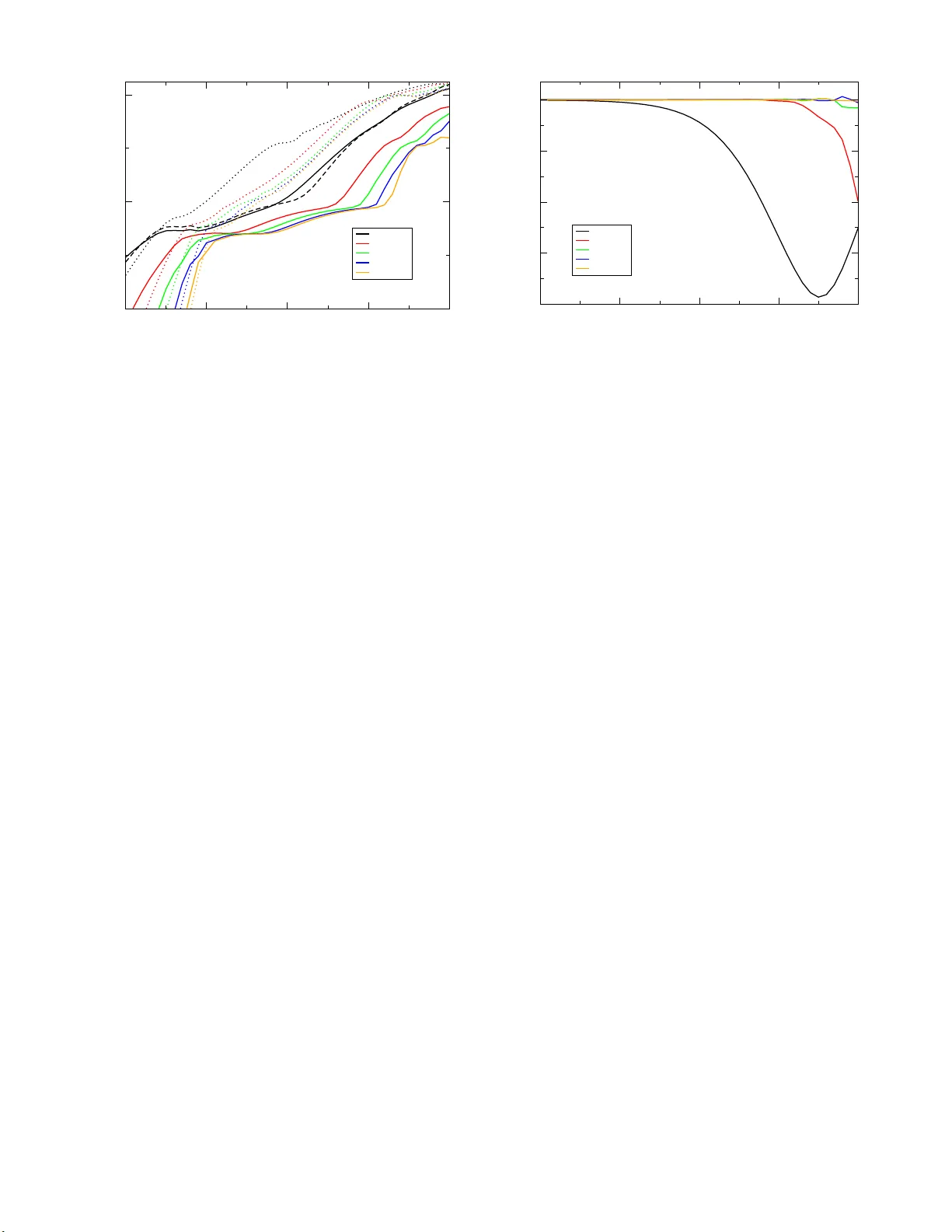
Efficien t w a v efunction propagation b y minimizing accum ulated action Zachary B. W alters 1 1 Max Born Institute, Ber eich B, Max Born St r asse 2a, 12489 Berlin A d lershof, Berlin Ge rmany (Dated: Marc h 25, 20 22) This pap er presents a new tec hnique to calculate the evolution of a qu antum w a vefunction in a chos en spatial basis by minimizing the accum ulated action. Introduction of a finite temp oral basis reduces the problem to a set of linear equations, while an appropriate choice of temp oral b asis set offers improv ed con vergence relative to metho ds based on matrix exp onentia tion for a class of physicall y relev an t problems. Calculating the time evolution of a quantum wav efunc- tion is a longstanding problem in co mputatio nal physics. The fundament al nature of the problem makes it resistant to s implifica tion. Pro blems of physical in terest, such as the in teractio n o f a mo lecule with a strong laser field, may lack symmetry or inv olve time dep endent, nonp erturba- tive fields. Problems inv olving mult iple dimensions or m ultiple in terac ting particles may q uic kly grow so lar ge as to be unma nageable with all but the largest c ompu- tational resour ces [1 – 3], a problem whic h is not e a sily outstripp ed by increases in computational p ow er. An ideal pro pagator, then, mu st s erve tw o masters – it must treat the physical side o f the problem accurately , and the computational side of the problem efficiently . The most co mmon approa ch to the pr oblem do es not treat the evolving wav efunction directly . Instead, the wa vef unction ψ ( x, t ) is expanded in some chosen basis s e t φ ( x, t ) = P i c i ( t ) χ i ( x ), where c i ( t 0 ) = h χ i | ψ ( t 0 ) i . Here ψ ( x, t ) is the true wa vefunction a nd φ ( x, t ) is its repre- sentation in the c hosen basis. After this expansio n has bee n made, the pro pagation scheme may op er a te only on the wav efunction’s representation, rather tha n the w av e- function itself. Within this gener al framework, there has been a great profusio n of metho ds for calcula ting the evolution o f the co efficients c i ( t ). Popular metho ds include Cra nk-Nicholson[4], s e cond order differencing[5], split op erator [6], short iterative La nczos[7], and Cheby- shev propa gation[8], as well as many others[9]. As may b e inferred fro m the la r ge n umber of com- peting metho ds, the practica l question of whic h metho d works b est is very difficult to answer, and us ua lly requires problem-sp ecific informa tio n. Ironically , the time dep en- dent Schr¨ odinger equation (TDSE), while challenging to solve, is not difficult to satisfy at a particular time. All of the ab ov e metho ds satisfy the TDSE exactly or ap- proximately at the initial time in the propag ation inter- v al. Indeed, entire families of pro pagators may satisfy the TDSE at the initial p oint: for the clas s of propaga - tors ψ ( x, t )(1 − iH α ∆ t ) = ψ ( x, t + ∆ t )( 1 + iH (1 − α ) ∆ t ), 0 ≤ ∆ t , the TDSE at time t is satisfied to first order for any v alue of α . α = 1 yields the forwards Euler metho d, α = 0 the backw ards Euler, α = 1 / 2 the Cra nk - Nic holso n. Although s uch metho ds may show shar p dif- ferences in s uita bilit y to particular problems, the TDSE alone gives little guidance. A full diagonaliza tion of the Hamiltonian matrix would satisfy the TDSE at all times; how ever, suc h a dia gonalizatio n would be prohibitively exp ensive for a large pr oblem, and would not ex ist for a problem with a time dep endent Hamiltonian. Compari- son of different propagato r s has often inv olved numerical testing on s imple problems[10, 11] or algor ithmic scaling arguments[12 ]. This pap er addresses the pro blem of w av efunction propaga tion from the physical p ersp ective of minimiz- ing the action acc umulated ov er the chosen time in terv al. Minimizing this a ction is shown to be equiv alent to mini- mizing the time integrated error of pr opagatio n. Because the action is c a lculated over the entire time s tep ra ther than at a single p oint, the constra in t that it be minimized is mor e strict than the TDSE, allowing the construction of a unique, v ariationally optimum propaga to r fo r a par- ticular or der in time. ERR ORS OF PR OP AGA TION AND REPRESENT A TION A central difficult y of any n umerical propag ation scheme is that, altho ugh the propaga to r se eks to mo del the ev olution o f an ideal wa vef unction ψ ( x, t ), it has ac- cess only to the r e presentation o f the wav efunction in some chosen basis, φ ( x, t ). The er ror of the r e presenta- tion is given by δ ( x, t ) = ψ ( x, t ) − φ ( x, t ). As a n a lternative to direct exp onentiation of the Hamiltonian, a propaga tor may b e constructed by mini- mizing the integral o f the err or ov er the time step Global err or = Z t +∆ t t dt ′ h δ ( x, t ′ ) | δ ( x, t ′ ) i . (1) W riting the error as a tw o term T a ylor s e ries, Global err or = Z t +∆ t t dt ′ h δ ( x, t ) | δ ( x, t ) i + Z t +∆ t t dt ′′ Z t ′ t d dt ′ h δ ( x, t ′ ) | δ ( x, t ′ ) i , (2) and recalling that i d dt ψ ( x, t ) = H ψ ( x, t ) fo r the true wa vef unction, the second term in equatio n 2 can b e w r it- 2 ten as d dt h δ ( x, t ) | δ ( x, t ) i = 2 i h φ ( x, t ) | ( i d dt − H ) | φ ( x, t ) i + 2 i h δ ( x, t ) | H | δ ( x, t ) i . (3) F rom equations 2 a nd 3, it is apparent that the global error may aris e either from imp erfectly re presenting the wa vef unction in a particula r basis (terms containing δ ( x, t )) or from imperfectly describing the evolution of the wav efunction in that bas is (terms containing φ ( x, t )). The r epresentation error ma y be minimized by an appro- priate choice of basis; here the focus is on minimizing the error o f pr opagatio n. The qua n tity h φ ( x, t ) | ( i d dt − H ) | φ ( x, t ) i found in eq ua- tion 3 is the Lagr a ngian density , and its integral over time gives the action accumulated b y the wav efunction in a particular interv al. Ho wev er, unlike the true Lagra ngian density , here the action is calculated with resp ect to the representation of the wav efunction, r ather than the wa ve- function itself. The dis tinction is significant. F or the true wa vefunction, minimizing the action is equiv alen t to setting i d dt ψ ( x, t ) − H ψ ( x, t ) = 0 for all x a nd t . F or the action minimizing representation of the wa v efunction, | h φ ( x, t ) | ( id/dt − H ) | φ ( x, t ) i | is dep endent o n the c hoice of spatial and tempor al basis functions and is no t guar- anteed to be zero. F or a finite basis of spatia l χ i ( x ) and temp or al T n ( t ) basis funct ions, a time dep enden t representation o f the wa vef unction can be written as φ ( x, t ) = X i,n C in χ i ( x ) T n ( t ) . (4) In this basis, the global erro r of Eq. 3 b ecomes a function of the co efficients C in and the matrix representations of the quantum mechanical oper ators. W riting the Hamilto- nian a s the sum of time indepe nden t and time dependent op erators H = H 0 ( x ) + V ( x, t ) (5) and defining the matrices H ij = Z dxχ ∗ i ( x ) H 0 χ j ( x ) (6) V ij nm = Z t +∆ t t dt ′ Z dxχ ∗ i ( x ) T ∗ n ( t ) V ( x, t ) χ j ( x ) T m ( t ) (7) O ij = Z dxχ ∗ i ( x ) χ j ( x ) (8) U nm = Z dtT ∗ n ( t ) T m ( t ) (9) Q nm = Z dtT ∗ ′ n ( t ) T m ( t ) , (10) the c hange in action res ulting from C in → C in + ǫ in is given by δ S = X i,j,n,m C in [ iO ij Q nm − H ij U nm − V ij nm ] ǫ ∗ j m (11) and the conditio n to minimize the a ccumulated action is that either ǫ ∗ j m = 0 (for the initial conditions ) or δ S j m = X i,n C in [ iO ij Q nm − H ij U nm − V ij nm ] ǫ ∗ j m = 0 (12) for all j,m. In these eq uations, i app earing as a subscr ipt is trea ted a s an index, while i multiplying O ij Q nm is the square ro ot of negative o ne. Equation 1 2 is the main r e s ult of this pa per . In order to co nstruct a least a ction propag a tor, it is necessa r y only to choos e a n appr o priate temp oral ba sis. While in principle this a nalysis applies equally well to any choice of ba s is, an obvious choice is for T n ( t ) to b e a set of linearly indep endent low-order p olyno mials in t. Lagra ng e in terp olating p olynomials pr ovide a con ve- nient se t o f tempora l basis functions. F or an evenly spaced grid t m = t + ∆ t ∗ m/n for m = 0 , n , the in- terp olating p olynomia ls a re given by T m ( t ) = Π k =0 ,n ; k 6 = m t − t k t m − t k . (13) This yields a basis set of n linea r ly indep endent n -o rder po lynomials in t, with the pro per t y tha t φ ( x, t n ) = P i C in χ i ( x ). O ne a dv antage of this choice of basis is that for small propag a tion times, C in will have compa- rable amplitudes for a ll n, making the asso ciated linear system easier to solve with high a ccuracy . Having chosen a temp oral basis , co e fficien ts C in which satisfy Equation 12 a s well as the initial condition C i 0 = h χ i | ψ ( t 0 ) i can b e found using Lag range m ultipliers. If S is the action a c c um ulated in the time interv al, let S ′ = S + P i λ i f ∗ i , wher e f i = C i 0 − h χ i | ψ ( t 0 ) i . The least action c o efficien ts are found b y minimizing S ′ with the constraint that f i = 0 for all i . This yields a system of linear equa tions X i,n C in [ iO ij Q nm − H ij U nm − V ij nm ] + λ j = 0 (14) for all j, m , and C i 0 = h χ i | ψ ( t 0 ) i (15) for all i . The Lagr ange m ultipliers λ j calculated in this pro cedure are not needed by the propa gator a nd can b e discarded after solving the linea r system. 3 COMP ARISON WITH THE LANCZOS PR OP AGA TOR The lea st actio n propag a tor derived in the previo us section is the unique, v ariatio nally optimum pro pa gator for a particular order in time. As suc h, it repres e n ts a fo rmal improvemen t ov er all propa gators approximat- ing the w av efunction as a low order po ly nomial in time – forward and ba ckw ards Euler, Crank Nic holson, sec- ond or der differencing, etc. Howev er, it is less clear how this formal improv ement translates to a pr actical bene fit, o r how the least action pr opagator compares to metho ds which a ttempt to diago nalize the Hamiltonian in a Krylov subspace, such as the p opular short iterative Lanczos metho d [7 ]. The Lanczos metho d works b y rep eatedly multiply- ing the initial wav efunction b y the Hamiltonian ma- trix to create a Krylov space of limited dimensio n in which the matrix exp onential e − iH t can b e calculated exactly . It is considered to be b oth efficient and quickly conv erging[10]. Existing v ariatio na l pr o pagator s have fo- cused on the evolution of the w av efunction in the Kr ylov subspace, yielding conv ergence pro per ties similar to the Lanczos propa gator[1 3, 14]. The Chebyshev propagato r, which also uses rep eated multiplication by the Hamilto- nian matr ix to cons truct a Krylov space, conv erges sim- ilarly to the Lanczos metho d[15 ]. In the limit that the Krylov space has dimension equal to the full Hamiltonia n, the Lanczos metho d is equiv alen t to diagonalizing the Hamiltonian, yielding L = i d dt ψ − H ψ = 0 at all times. This solution is the globa l minimum action solution, and cannot be improved upo n. Ho wev er, for most applica tions, the Krylov subspace is chosen to hav e a muc h smaller o rder – typically in the range 1-1 0. Because the Kr ylov subspace is constructed through rep eatedly multiplying a n initial w av efunction by the Hamiltonian matrix, later Kry lov basis vectors will tend to some ov erlap with those eigenv ectors of H with the largest e ig env alues. F or problems with Coulomb sing u- larities o r fine spatial ba s es, it is not uncommon fo r these largest eigenv alues to b e artifacts o f the ch oice of ba- sis, having no counterpart in the system being describ ed. How ev er, they may nonetheless ser ve to limit the stepsize which may be taken with high a ccuracy . If an idea l w av efunction (ie, without reference to a ba- sis) ψ ( x, t ) ca n b e expanded in terms o f ener g y eigenfunc- tions ov er a sho rt time interv al ψ ( x, t ) = X α c α f α ( x ) e − iE α ( t − t 0 ) (16) and the evolution of the w av efunction’s r epresentation in the Kr ylov subspace is given by φ ( x, t ) = X β d α,β g β ( x ) e − iE β ( t − t 0 ) , (17) where d α,β = c α h g β | f α i , then the erro r is given b y δ ( x, t ) = X α,β d α,β g β ( x )( e − iE α ( t − t 0 ) − e − iE β ( t − t 0 ) ) (1 8) and h δ | δ i = X α,β | d α,β | 2 4 s in 2 ( E α − E β 2 ( t − t 0 )) . (19) If the Kr ylov subspac e is now partitioned into a “g o o d” subspace with E β < E cutoff and a “ba d” subs pa ce with E β > E cutoff , the error can b e estimated by setting E α − E β = 0 in the go o d subs pa ce and E β − E α = E H , where E H reflects the largest eigenv a lues of H, yielding h δ | δ i ≈ X α,β ,E β >E cutoff | d α,β | 2 4 s in 2 ( 1 2 E H ( t − t 0 )) . (20) The error of the Lanczos metho d is thus minimized either when the pr o jection into the bad subspac e is small or when E H ∆ t << 1. In cont ras t to the Lanczo s metho d, the erro r of the least actio n propagator is b ounded by the error of the T aylor s eries of the true wa vefunction. Th us h δ | δ i ≤ X α | c α | 2 | e − iE α ( t − t 0 ) − N max X n =0 ( − iE α ) n n ! ( t − t 0 ) n | 2 (21) and the conditio n for the error to rema in small is s imply that E cutoff ∆ t < 1. F or a pro blem with E cutoff << E H , the lea st action propaga tor offers the p ossibility of muc h larger stepsizes at high accur acy than the Lanczos prop- agator . The tw o pro pagator s were tested numerically using a 1 dimensiona l Coulomb p otent ial 1 /x for x ranging from 0 to 10 . The regio n was separ a ted into 100 finite el- ement reg ions, with tw o quadra tic finite elements per region. The wa vefunction was restr ic ted to have zer o v alue at b oth endp oints. The largest eigenv alue of the resulting Hamiltonian matrix was 4 9 9 Ha r tree. The ini- tial wav efunction was c hosen to b e a Ga ussian of unit width, cent ered at x = 2. The choice of initial wav efunc- tion and p otential w ere ma de to ensure that the wav e- function would b e far from equilibrium and hav e a strong int erac tio n with the Coulo mb p otential, a s for an electro n wa vepac ket sca ttering from a po sitive ion. The accura cy of the Lanczos - and least action pr opa- gator was calculated by pro pa gating the initial w av efunc- tion a sing le timestep and comparing the resulting wa ve- function with the “ true” wa vefunction found by directly diagonalizing the full Hamiltonian. yielding an error | err | = h δ ( t + δ t ) | δ ( t + δ t ) i . (22) F or the least action propaga tor, the or der of propag ation is o ne less than the degree o f the p o lynomial basis func- tions. F or the La nczos propa gator, the or der is given by 4 -3 -2 -1 0 1 log 10 dt -10 -5 0 log 10 err 1st order 3rd order 5th order 7th order 9th order FIG. 1. (Color online) Poin t error h δ ( x, t + ∆ t ) | δ ( x, t + ∆ t ) i of Crank N ic holson (dashed line), Lanczos (dotted lines) and least action (solid lines) propagators, as a function of step size. F or large stepsizes, the least action propagator is many times more accurate than the Lanczos p ropagator of the same order. the dimensio n of the Kr ylov subspace, starting with 0 for the initial wa vef unction. The error a s a function of order and stepsize for the t wo metho ds is shown in Figur e 1. Also shown in the fig- ure is the error vs time for the p opular Cra nk Nicholson first order propa gator [4]. As opp osed to the global err o r which was used in the deriv ation of the least action prop- agator , these figur es s how the p oint erro r after a single propaga tion step. These results show that the le a st a ction pr opagator of- fers the potential for larg e timesteps to b e taken with high a ccuracy , with the greatest a dv an tage coming from propaga tion at hig h order . At first or der, the lea st action propaga tor g ives approximately the same p oint erro r as the Cr a nk Nicholson metho d, while hig her or ders rapidly decrease the error for a particular timestep, or alterna- tively increase the s iz e of the timestep which can b e taken for a particula r desired err o r. As the order increa ses, the error b egins to saturate as differen t or der pr opagator s conv erge o n the same result. That this sa turation do es not result in zero error may re sult from numerical error in the diago na lization o f the Hamiltonian or the linear solver. F or all or de r s tested, the least action propa gator was many times mor e accura te than the Lanczo s propag ator for large stepsizes. F o r very sma ll stepsizes, the erro r of bo th metho ds was co mpa rable, with the Lanczos metho d more accurate. Both metho ds beca me m uch more accu- rate for stepsize s o f less than 10 − 2 , which is interpreted to mean that the initial w av efunction had so me pro jec- tion o n to very high energy eigenstates ; ie, the sample problem did not hav e E cutoff << E H . One weakness of the least ac tio n propag ators which -3 -2 -1 0 1 log 10 dt -0.08 -0.06 -0.04 -0.02 0 (log 10 |norm|) / dt 1st order 3rd order 5th order 7th order 9th order FIG. 2. (Color online) Ex p onentia l gro wth rate (log 10 | norm | ) /dt v s p ropagation time for different or- ders of the least action p ropagator. Higher orders show a gro wth rate closer to zero. arises from the choice o f p olynomial basis functions is that the no r m o f the propagated wa vefunction is not required to b e a cons tan t as a function of time. Fig - ure 2 shows the ra te of gr owth/deca y of the nor m h φ | φ i for different or ders of propag ation as a function of step size. Here the la rgest deviation from zero growth r ate is found for the combination of low order and lar ge step- size. Higher order propaga tors sho w growth rates close to zero. F or problems r equiring re p ea ted use o f the prop- agator ov er many timesteps, it is thus likely that the propaga ted w av efunction will need to be renormalized per io dically . Because the norm is still very clo se to 1, such renor ma lization has a minimal effect on the p oint error shown in Figure 1. F rom these figur es, it is appa r ent that the leas t a c- tion pr o pagator works bes t a t high o rders, which offer the combination of large time s teps , high accura cy a nd low rates of growth o r decay of the nor m. Ho wev er, high order a lso incr eases the size of the linear system w hich m ust b e solved at each step. F or a basis consisting of n x spatial and n t tempo ral basis functions, the lea st action propaga tor r equires n s = n x ( n t + 1) v ariables to b e solved for. While s pecific implementations are b eyond the sco pe of this pap er , the question of how be st to solve this linear system will play a crucia l role in applying the least action propaga tor to rea l world problems. T o this end, a few fea- tures of the least action linear s y stem are worth noting. First among these is the highly separable nature of the least action linear system defined in equations 14 and 1 5. In equation 1 4, the v ariation o f the action is given a s the sum of three ma trices, O ij Q nm , H ij U nm , and V ij nm . Of these, the first t wo a re separ ated into the pro duct of spa - tial and tempor al matrices. Beca use of this, these tw o matrices inherit the sparsity and/o r banded structure o f the underlying spatial matrices. The case is similar for 5 the nons eparable V ij nm : the integral ov er time and s pace is nonzero o nly if the in tegral over space is nonzer o. Be- cause o f this, ba s is s ets such as finite elements which are chosen for the structure of their Ha milto nia n and ov erlap matrices will retain these adv antages in the least action equation. F or a banded problem such as the 1D finite element problem trea ted in this pap er, the ba ndwidth of the linear system increas e s linearly with the order of the propaga tor, giv ing an overall n 2 t scaling with the or der. F or very large pr o blems which lack such a simple struc- ture, it is likely that solutio n of the lea st action linear sy s- tem will requir e use of an iterative s o lver, such a s those av ailable in the PE TSc [16] or T rilinos [17] libraries. Suc h solvers, require calculating a matr ix vector pro duct at every iteration. Here the adv an tages o f the leas t action equation’s s eparable form are very apparent, par ticula rly in the ca se of a static Hamiltonia n. A single matrix vector pro duct of the linea r system defined in eq uations 14 a nd 15 r e q uires 1 (very expens ive) matrix-vector m ultiplica- tion by the unseparated matrix V ij nm , 2 n t independent (exp e ns ive) multiplications of the form D im = M ij C j m , where M = O or H , follow ed by 2 n x (ch eap) indepen- dent m ultiplications of the form F in = N nm D im , where N = Q or U . Thus, although the linear system which m ust be solved is v ery large, it is well suited to itera- tive solution. The ov erall sc aling of one iteration with resp ect to pr opagator order will b e limited by the slow- est of these steps, which may depend on sp ecifics of the data structure and ar chit ecture of the system us e d. This pap er has addr e ssed the problem of pro pagating a wa vef unction in time by minimizing he accumulated action. F or a pa r ticular choice of s patial and tempo- ral basis functions , the problem is reduced to solution of a (potentially very la rge) system of linear eq uations. This linear system inherits the sparsity and/ or banded structure of the spatial Hamiltonian and overlap matr i- ces, while its separable structure ma kes it amena ble to solution by iterative solvers. The res ulting propag ator was shown to hav e improv ed conv ergence rela tive to the commonly used sho r t iterative Lanczo s propagato r, giv- ing the p otential for larger stepsizes at high accur acy . The der iv ation of the action as a mea sure of propaga - tion erro r is a powerful r esult which offers many opp or- tunities for the systematic improv ement of pro pagation schemes. By monitoring the spacetime v olumes where the mo s t action is accumulated, spatial or tempo ral ba ses could be selectively refined to increas e the total accura cy of a pr opagation step at minimal additional co mputa- tional effort. F o r this rea s on, the full p ow er of the a ction minimization pr inciple may b e yet to be unlo ck ed. [1] T a ylor, K. et al., Journal of Electron Sp ectroscopy and Related Ph enomena 144 (2005) 1191. [2] F eis t, J. et al., Physical review letters 103 (2009) 63002. [3] Sansone, G. et al., Nature 465 763. [4] Crank, J. and Nicolson, P ., Adv ances in Computational Mathematics 6 (1996) 207. [5] Aska r, A. and Cakmak, A ., The Journal of Chemical Physics 68 (1978) 2794. [6] Bandrauk, A. and Shen, H., Chemical Physics Letters 176 (1991) 428. [7] Park, T. and Light, J., The Journal of c hemical physics 85 (1986) 5870. [8] T a l-Ezer, H. and Kosloff, R ., The Journal of Chemical Physics 81 (1984) 3967. [9] Moler, C. and V an Loan, C., S IAM review 45 (2003) 3. [10] Leforestier, C. et al., Journal of computational physics 94 (1991) 59. [11] T ru ong, T. et al., The Journal of Chemical Physics 96 (1992) 2077. [12] Kosloff, R., The Journal of Physical Chemistry 92 (1988) 2087. [13] T riozon, F., Roche, S., and May ou, D., Riken Review (2000) 73. [14] T al-Ezer, H ., Kosloff, R., and Cerjan, C., Journal of Computational Ph ysics 100 (1992) 179. [15] Chen, R . and Guo, H., The Journal of Chemical Physic s 119 (2003) 5762. [16] Bala y , S. et al., (2003). [17] Heroux, M. et al., ACM T ransactio ns on Mathematical Soft ware (TOMS) 31 (2005) 397.