Practical recipes for the model order reduction, dynamical simulation, and compressive sampling of large-scale open quantum systems

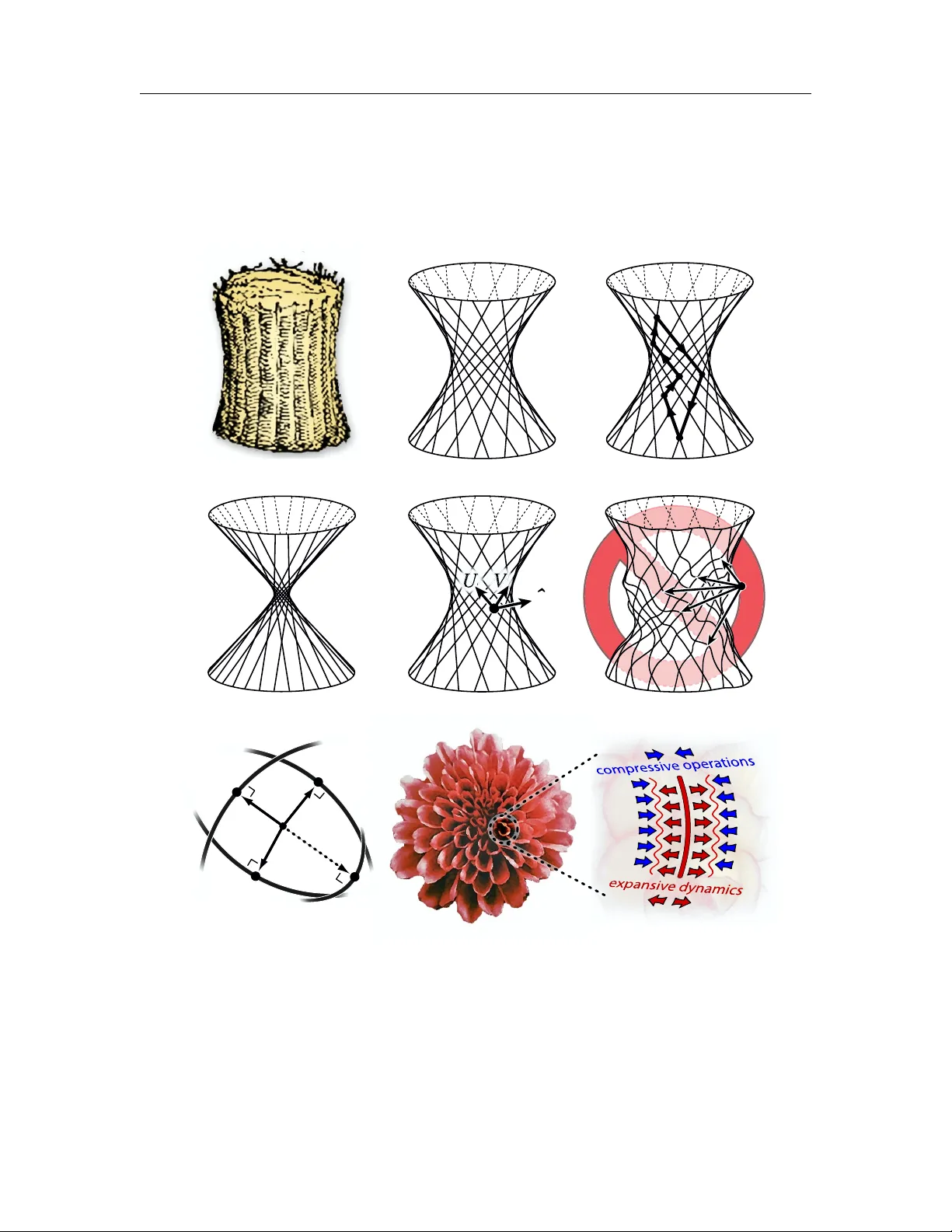
Practical recip es for the mo del order reduction, dynamical sim ulation, and compressiv e sampling of large-scale op en quan tum systems J. A. Sidles ∗ 1 , J. L. Garbini 2 , L. E. Harrell 3 , A. O. Hero 4 , J. P . Jac ky 1 , J. R. Malcom b 2 , A. G. Norman 5 , A. M. Williamson 2 Octob er 24, 2018 This article presen ts practical numerical recip es for simulating high-temp erature and non- equilibrium quan tum spin systems that are con tinuously measured and controlled. The no- tion of a “spin system” is broadly conceiv ed, in order to encompass macroscopic test masses as the limiting case of large- j spins. The sim ulation technique has three stages: ﬁrst the delib erate in tro duction of noise into the sim ulation, then the con v ersion of that noise into an informatically equiv alen t contin uous measurement and con trol pro cess, and ﬁnally , pro jec- tion of the tra jectory onto a K¨ ahlerian state-space manifold having reduced dimensionalit y and p ossessing a K¨ ahler p oten tial of multilinear ( i.e. , pro duct-sum) functional form. These state-spaces can b e regarded as ruled algebraic v arieties up on which a pro jectiv e quantum mo del order reduction ( QMOR ) is p erformed. The Riemannian sectional curv ature of ruled K¨ ahlerian v arieties is analyzed, and pro ved to b e non-p ositive upon all sections that con tain a rule. It is further shown that the class of ruled K¨ ahlerian state-spaces includes the Slater determinan t wa ve-functions of quan tum c hemistry as a sp ecial case, and that these Slater determinan t manifolds hav e a F ubini-Study metric that is K¨ ahler-Einstein; hence they are solitons under Ricci ﬂo w. It is suggested that these negativ e sectional curv ature prop er- ties geometrically account for the ﬁdelity , eﬃciency , and robustness of pro jective tra jectory sim ulation on ruled K¨ ahlerian state-spaces. Some implications of tra jectory compression for geometric quan tum mechanics are discussed. The resulting sim ulation formalism is used to construct a p ositive P -represen tation for the thermal densit y matrix and to derive a quantum limit for force noise and measurement noise in monitoring b oth macroscopic and microscopic test-masses; this quan tum noise limit is shown to b e consistent with well- established quan tum noise limits for linear ampliﬁers and for monitoring linear dynamical systems. Single-spin detection b y magnetic resonance force microscopy ( MRFM ) is then sim ulated, and the data statistics are sho wn to b e those of a random telegraph signal with additiv e white noise, to all orders, in excellent agreemen t with exp erimental results. Then a larger-scale spin-dust mo del is simulated, ha ving no spatial symmetry and no spatial ordering; the high-ﬁdelit y pro jection of n umerically computed quan tum tra jectories onto lo w-dimensionality K¨ ahler state-space manifolds is demonstrated. Finally , the high-ﬁdelity reconstruction of quantum tra jectories from sparse random pro jections is demonstrated, the onset of Donoho-Sto dden breakdown at the Cand` es-T ao sparsity limit is observed, and metho ds for quan tum state optimization b y Dantzig selection are given. ∗ T o whom corresp ondence should be addressed. 1 Dept. of Orthopædics and Sp orts Medicine, Box 356500, Sc hool of Medicine, Universit y of W ashington, Seattle, W ashington, USA; 2 Dept. of Mechanical Engineering, Univ ersity of W ashington; 3 Dept. of Physics, U. S. Military Academy , W est Poin t; 4 Dept. of Electrical Engineering, Univ ersity of Michigan; 5 Dept. of Bio engineering, Universit y of W ashington Con ten ts 1 In tro duction 6 1.1 Ho w do es the Stern-Gerlac h eﬀect r e al ly work? . . . . . . . . . . . . . 6 1.1.1 Constrain ts up on the analysis . . . . . . . . . . . . . . . . . . . 6 1.2 The feasibilit y of generic large-s cale quan tum simulation . . . . . . . . 6 1.2.1 The geometry of reduced-order state-spaces . . . . . . . . . . . 7 1.2.2 The cen tral role of cov ert measurements . . . . . . . . . . . . . 7 1.2.3 Bac kground assumed by the presentation . . . . . . . . . . . . . 7 1.2.4 Ov erview of the analysis and sim ulation recip es . . . . . . . . . 7 1.3 Ov erview of the formal simulation algorithm . . . . . . . . . . . . . . . 7 1.3.1 The op erational approac h to quan tum simulation . . . . . . . . 9 1.3.2 The em brace of quantum ortho do xy . . . . . . . . . . . . . . . . 9 1.3.3 The unitary in v ariance of quantum op erations . . . . . . . . . . 9 1.3.4 Naming and applying the The or ema Dile ctum . . . . . . . . . . 10 1.3.5 Relation to geometric quan tum me c hanics . . . . . . . . . . . . 10 1.4 Ov erview of the numerical simulation algorithm . . . . . . . . . . . . . 11 1.4.1 The main ideas of pro jective mo del order reduction . . . . . . . 11 1.4.2 The natural emergence of K¨ ahlerian geometry . . . . . . . . . . 11 1.4.3 Preparing for a K¨ ahlerian geometric analysis . . . . . . . . . . . 13 1.5 Ov erview of the unifying geometric ideas . . . . . . . . . . . . . . . . . 13 1.5.1 The algebraic structure of the reduced-order state space . . . . 13 1.5.2 The mediev al idea of a gabion, and its mathematical parallels . 15 1.5.3 The geometric prop erties of gabion-K¨ ahler ( GK ) manifolds . . . 16 1.5.4 GK manifolds are endo wed with rule ﬁelds . . . . . . . . . . . . 18 1.5.5 GK geometry has singularities . . . . . . . . . . . . . . . . . . . 18 1.5.6 GK pro jection yields compressed representations . . . . . . . . . 18 1.5.7 GK manifolds ha ve negative sectional curv ature . . . . . . . . . 18 1.5.8 GK manifolds ha ve an eﬄorescing global geometry . . . . . . . 19 1.5.9 GK basis v ectors are ov er-complete . . . . . . . . . . . . . . . . 19 1.5.10 GK manifolds allo w eﬃcient algebraic computations . . . . . . . 19 1.5.11 GK manifolds supp ort the The or ema Dile ctum . . . . . . . . . . 19 1.5.12 GK manifolds supp ort thermal equilibria . . . . . . . . . . . . . 20 1.5.13 GK manifolds supp ort fermionic states . . . . . . . . . . . . . . 20 1.6 Ov erview of contrasts b et ween quantum and classical simulation . . . 21 1.6.1 The The or ema Dile ctum is fundamen tal and universal . . . . . . 21 1.6.2 Quan tum state-spaces are veiled . . . . . . . . . . . . . . . . . . 21 1.6.3 Noise mak es quantum simulation easier . . . . . . . . . . . . . . 21 1.6.4 K¨ ahlerian manifolds are geometrically sp ecial . . . . . . . . . . 21 2 The sectional curv ature of gabion–K¨ ahler ( GK ) state-spaces 22 2.1 Quan tum MOR state-spaces viewed as manifolds . . . . . . . . . . . . 22 2.1.1 Deﬁning gabion pseudo-co ordinates . . . . . . . . . . . . . . . . 23 2.2 Regarding gabion manifolds as real manifolds . . . . . . . . . . . . . . 23 2.2.1 Constructing the metric tensor . . . . . . . . . . . . . . . . . . . 24 2.2.2 Raising and lo wering the indices of a pse udo-co ordinate basis . 24 2.2.3 Constructing pro jection op erators in the tangent space . . . . . 24 2.3 “Push-button” strategies for curv ature analysis . . . . . . . . . . . . . 24 2.3.1 The deﬁciencies of push-button curv ature analysis . . . . . . . . 25 2 CONTENTS 3 2.4 The sectional curv ature of gabion state-spaces . . . . . . . . . . . . . . 25 2.4.1 Remarks on gabion normal v ectors . . . . . . . . . . . . . . . . 25 2.4.2 Computing the directed sectional curv ature . . . . . . . . . . . 25 2.4.3 Ph ysical interpretation of the directed sectional curv ature . . . 26 2.4.4 Deﬁnition of the in trinsic sectional curv ature . . . . . . . . . . . 26 2.5 The formal deﬁnition of a gabion manifold . . . . . . . . . . . . . . . . 27 2.5.1 Recip es for constructing rules and rule ﬁelds . . . . . . . . . . . 28 2.5.2 The set of gabion rules is geo desically complete . . . . . . . . . 28 2.6 Gabion-K¨ ahler ( GK ) manifolds . . . . . . . . . . . . . . . . . . . . . . 28 2.6.1 K¨ ahlerian indexing and co ordinate conv entions . . . . . . . . . 28 2.6.2 GK sectional curv ature in physics bra-ket notation . . . . . . . 30 2.6.3 Deﬁning the Riemann curv ature tensor . . . . . . . . . . . . . . 30 2.6.4 The The or ema Egr e gium on GK manifolds . . . . . . . . . . . . 31 2.6.5 Readings in K¨ ahlerian geometry . . . . . . . . . . . . . . . . . . 32 2.7 Remarks up on holomorphic bisectional curv ature . . . . . . . . . . . . 32 2.7.1 Relation of Theorem 2.1 to the HBCN Theorem . . . . . . . . . 33 2.7.2 Practical implications of sectional curv ature theorems . . . . . . 33 2.8 Analytic gold standards for GK curv ature calculations . . . . . . . . . 33 2.9 The Riemann-K¨ ahler curv ature of Slater determinan ts . . . . . . . . . 34 2.10 Slater determinan ts are Grassmannian GK ( GGK ) manifolds . . . . . . 37 2.11 Practical curv ature calculations for QMOR on GK manifolds . . . . . . 37 2.12 Numerical results for pro jective QMOR onto GK manifolds . . . . . . . 38 2.13 Av enues for research in geometric quantum mechanics . . . . . . . . . 40 2.14 Summary of the geometric analysis . . . . . . . . . . . . . . . . . . . . 41 3 Designing and Implementing Large-Scale Quantum Sim ulations 41 3.1 Organization and nomenclature of the presen tation . . . . . . . . . . . 42 3.2 QMOR resp ects the principles of quan tum mec hanics . . . . . . . . . . 42 3.2.1 QMOR resp ects the The or ema Dile ctum . . . . . . . . . . . . . 42 3.2.2 QMOR resp ects thermal equilibrium . . . . . . . . . . . . . . . 44 3.2.3 QMOR resp ects classical linear con trol theory . . . . . . . . . . 47 3.2.4 Remarks up on the sp o oky mysteries of classical physics . . . . . 49 3.2.5 Exp erimen tal proto cols for measuring the Hilb ert parameters . 51 3.2.6 QMOR sim ulations resp ect the fundamen tal quantum limits . . 52 3.2.7 T eac hing the ontological ambiguit y of classical measurement . . 54 3.3 Ph ysical asp ects of QMOR . . . . . . . . . . . . . . . . . . . . . . . . . 54 3.3.1 Measuremen t mo deled as scattering . . . . . . . . . . . . . . . . 55 3.3.2 Ph ysical and mathematical descriptions of in terferometry . . . . 55 3.3.3 Surv ey of interferometric measurement metho ds . . . . . . . . . 55 3.3.4 Ph ysical calibration of scattering amplitudes . . . . . . . . . . . 56 3.3.5 Noise-induced Stark shifts and renormalization . . . . . . . . . . 58 3.3.6 Causalit y and the The or ema Dile ctum . . . . . . . . . . . . . . 59 3.3.7 The The or ema Dile ctum in the literature . . . . . . . . . . . . . 59 3.4 Designs for spinometers . . . . . . . . . . . . . . . . . . . . . . . . . . 60 3.4.1 Spinometer tuning options: ergo dic, synoptic, and batrachian . 60 3.4.2 Spinometers as agen ts of tra jectory compression . . . . . . . . . 61 3.4.3 Spinometers that einselect eigenstates . . . . . . . . . . . . . . . 61 3.4.4 Con vergence b ounds for the einselection of eigenstates . . . . . 62 3.4.5 T riaxial spinometers . . . . . . . . . . . . . . . . . . . . . . . . 63 CONTENTS 4 3.4.6 The Blo c h equations for general triaxial spinometers . . . . . . 63 3.4.7 The einselection of coheren t states . . . . . . . . . . . . . . . . . 63 3.4.8 Con vergence b ounds for the einselection of coheren t states . . . 65 3.4.9 Implications of einselection b ounds for quan tum sim ulations . . 66 3.4.10 P ositive P -represen tations of the thermal density matrix . . . . 66 3.4.11 The spin-1/2 thermal equilibrium Blo c h equations . . . . . . . . 67 3.4.12 The spinometric Itˆ o and F okker-Planc k equations . . . . . . . . 67 3.4.13 The standard quan tum limits to linear measurement . . . . . . 69 3.4.14 Multiple expressions of the quan tum noise limit . . . . . . . . . 70 3.5 Summary of the design rules . . . . . . . . . . . . . . . . . . . . . . . . 70 4 Examples of quantum sim ulation 70 4.1 Calibrating practical sim ulations . . . . . . . . . . . . . . . . . . . . . 71 4.1.1 Calibrating the Blo c h equations . . . . . . . . . . . . . . . . . . 71 4.1.2 Calibrating test-mass dynamics in practical sim ulations . . . . . 72 4.1.3 Calibrating purely observ ation pro cesses . . . . . . . . . . . . . 72 4.2 Three single-spin MRFM sim ulations . . . . . . . . . . . . . . . . . . . 73 4.2.1 A batrac hian single-spin unrav eling . . . . . . . . . . . . . . . . 74 4.2.2 An ergo dic single-spin unra v elling . . . . . . . . . . . . . . . . . 74 4.2.3 A synoptic single-spin unra velling . . . . . . . . . . . . . . . . . 74 4.3 So ho w do es the Stern-Gerlac h eﬀect r e al ly work? . . . . . . . . . . . . 75 4.4 W as the IBM can tilever a macroscopic quantum ob ject? . . . . . . . . 75 4.5 The ﬁdelit y of pro jectiv e QMOR in spin-dust sim ulations . . . . . . . . 76 4.5.1 The ﬁdelit y of quantum state pro jection on to GK manifolds . . 76 4.5.2 The ﬁdelit y of spin p olarization in pro jective QMOR . . . . . . 77 4.5.3 The ﬁdelit y of op erator co v ariance in pro jectiv e QMOR . . . . . 78 4.5.4 The ﬁdelit y of quantum concurrence in pro jectiv e QMOR . . . . 78 4.5.5 The ﬁdelit y of mutual information in pro jectiv e QMOR . . . . . 79 4.6 Quan tum state reconstruction from sparse random pro jections . . . . . 79 4.6.1 Establishing that quan tum states are compressible ob jects . . . 80 4.6.2 Randomly pro jected GK manifolds are GK manifolds . . . . . . 81 4.6.3 Donoho-Sto ddard breakdo wn at the Cand ` es-T ao b ound . . . . . 82 4.6.4 W edge pro ducts are Hamming metrics on GK manifolds . . . . 84 4.6.5 The n and p dimensions of deterministic sampling matrices . . . 85 4.6.6 P etal-counting in GK geometry via co ding theory . . . . . . . . 86 4.6.7 Constructing a Dan tzig selector for quan tum states . . . . . . . 87 4.6.8 RIP prop erties of deterministic v ersus random sampling matrices 88 4.6.9 Wh y do CS principles work in QMOR simulations? . . . . . . . 89 5 Conclusions 90 5.1 Concrete applications of large-scale quan tum sim ulation . . . . . . . . 91 5.1.1 The goal of atomic-resolution biomicroscop y . . . . . . . . . . . 91 5.2 The acceleration of classical and quan tum sim ulation capability . . . . 92 5.3 The practical realities of quan tum system engineering in MRFM . . . . 93 5.4 F uture roles for large-scale quan tum simulation . . . . . . . . . . . . . 93 List of Figures 1 F ormal algorithm for quan tum mo del order reduction ( QMOR ) . . . . . . . 8 2 Numerical algorithm for quan tum mo del order reduction ( QMOR ) . . . . . 12 3 Algebraic deﬁnition of a gabion-K¨ ahler ( GK ) state-space . . . . . . . . . . . 14 4 Geometric principles of quan tum mo del order reduction ( QMOR ) . . . . . . 17 5 T ypical Ricci tensor eigenv alues for gabion-K¨ ahler manifolds . . . . . . . . 38 6 The three k ernel classes of linear, classical QMOR simulations . . . . . . . . 48 7 Three design rules that reﬂect “sp o oky classical physics” . . . . . . . . . . . 50 8 Three asp ects of photon in terferometry . . . . . . . . . . . . . . . . . . . . . 56 9 A ph ysical embo dimen t of the The or ema Dile ctum . . . . . . . . . . . . . . 57 10 Sim ulation of single electron moment detection by MRFM . . . . . . . . . . 73 11 The dep endence of QMOR ﬁdelit y up on GK order and rank . . . . . . . . . 77 12 Measures of pro jective ﬁdelity . . . . . . . . . . . . . . . . . . . . . . . . . . 78 13 Quan tum state reconstruction from sparse random pro jections . . . . . . . 83 List of T ables 1 Recip es for deterministic construction of sampling matrices . . . . . . . . . 86 2 RIP prop erties of deterministic v ersus random 8 × 16 sampling matrices . . 88 5 6 1. Intro duction This article describ es practical recip es for the sim ulation of large-scale op en quantum spin systems. Our ov erall ob jective is to enable the reader to design and implemen t practical quan tum sim ulations, guided by an appreciation of the geometric, informatic, and algebraic principles that go vern simulation accuracy , robustness, and eﬃciency . 1.1. How do es the Stern-Gerlach eﬀe ct really work? This article had its origin in a question that Dan Rugar asked of us about ﬁv e y ears ago: “Ho w does the Stern-Gerlac h Eﬀect r e al ly work?” The w ord “ r e al ly ” is notew orthy because h undreds of articles and b o oks on the Stern-Gerlach eﬀect hav e b een written since the orig- inal exp erimen ts in 1921 [88, 89, 90] . . . including articles b y the authors [178, 182] and b y Dan Rugar [179] himself. Y et w e were unable to ﬁnd, within this large literature, an answ er that w as satisfactory in the context in which the question w as ask ed, that circum- stance b eing the (ultimately successful) endeav or by Rugar’s IBM research group to detect the magnetic momen t of a single e lectron spin b y magnetic resonance force microscopy ( MRFM ) [170]. 1.1.1. Constr aints up on the analysis Quan tum theory has a reputation for m ystery . But as Peter Shor has remarked, “Interpretations of quan tum mechanics, unlik e Go ds, are not jealous, and thus it is safe to b eliev e in more than one at the same time.” In particular, it is well known—and w e will review the literature in this article—that adv ances in quantum information theory ha ve provided Shor’s principle with rigorous foundations. W e will build up on these informatic foundations in answering Dan Rugar’s question in accord with the follo wing constraints: our analysis will be ortho dox in its resp ect for established principles of quan tum physics. It will b e op er ational in the sense that all its predictions are traceable to explicitly hardw are-based measurement processes. The analysis will b e sc alable to accommo date large-dimension quantum systems (such as the spins in protein molecules that are the ultimate targets of MRFM microscopy). The analysis will b e r e ductive in the sense that the analysis will yield simple design rules that are in reasonable quan titative accord with the predictions of more accurate—but more complicated—large- scale n umerical simulations. The analysis will b e synoptic in the sense that when w e are required to choose b et w een equiv alent analysis formalisms, a rationale for these choices will b e provided, and the consequences of alternative c hoices noted. And ﬁnally , the analysis will b e extensible —at least in principle—to the analysis and simulation of general quantum systems (suc h as spintronic devices, nanomechanical devices, and biomolecules). There are of course strong practical motiv ations for seeking to analyze quan tum systems b y metho ds that are ortho do x, op erational, scalable, reductive, synoptic, and extensible: these same attributes are essential to practical metho ds for analyzing large-scale classical systems [20, 113]. 1.2. The fe asibility of generic lar ge-sc ale quantum simulation W e did not b egin our inv estigations with the idea that the n umerical simulation of large-scale quan tum spin systems w as feasible. Indeed, w e were under the opp osite impression, based up on the no-sim ulation argumen ts of F eynman [67] in the early 1980s. These arguments ha ve b een widely—and usually uncritically—rep eated in textb o oks [146, sec. 4.7]. But F eynman’s arguments do not formally apply to noisy systems, and in the course of our analysis, it became apparent that this pro vides a loophole for dev eloping eﬃcien t sim ulation algorithms. F urthermore, it b ecame apparent that the class of noisy systems encompasses as a sp ecial case the low-temperature and strongly correlated systems that are studied in quan tum chemistry and condensed matter physics. In the concluding section of this article 1.3 Ov erview of the formal simulation algorithm 7 (Section 4.6), w e will develop the p oin t of view that any quantum state that has b een in con tact with a thermal reserv oir is an algorithmically compressible ob ject. This lo ophole help ed us understand why—from an empirical p oint of view—sim ulation capabilities in quantum chemistry and condensed matter physics hav e been improving ex- p onen tially in recent decades [80, 149, 151]. The analysis and sim ulation metho ds that we will presen t in this article broadly deﬁne a geometric and quantum informatic program for sustaining this progress. 1.2.1. The ge ometry of r e duc e d-or der state-sp ac es This article’s mathematical methods are no vel mainly in their fo cus up on the geometry of reduced-order quantum state-spaces. W e will show that the quantum state-spaces that are most useful for large-scale simulation purp oses generically hav e an algebraic structure that can be geometrically in terpreted as a net w ork of geo desic curv es (rules) having nonp ositive Gaussian curv ature for all sections that contain a rule (Section 2). W e will see that these curv ature prop erties are essential to the eﬃciency and robustness of mo del order reduction. 1.2.2. The c entr al r ole of c overt me asur ements A technique that is cen tral to our sim ula- tion recip es is to sim ulate all noise pro cesses (including thermal baths) as equiv alen t cov ert measuremen t and con trol pro cesses (Section 3). F rom a quantum informatic p oin t of view, co vert quan tum measurement processes act to quenc h high-order quantum correlations that otherwise w ould b e infeasibly costly to compute and store (Section 4). Thus the presence of noise can allo w quan tum sim ulations to ev ade the no-simulation arguments of F eynman [67]. 1.2.3. Backgr ound assume d by the pr esentation No reader will b e expert in all of the disciplines that our analysis and sim ulation recip es em b o dy , whic h are (c hieﬂy) quantum mec hanics in b oth its ph ysical and informatic asp ects, the engineering theory of mo del order reduction ( MOR ) and dynamical con trol, and the mathematical to ols and theorems of algebraic and diﬀeren tial geometry . Indeed, the writing this article has made the authors acutely aw are of their own considerable deﬁciencies in all of these areas. Recognizing this, we will describ e all asp ects of our recip es at a lev el that is intended to b e broadly comprehensible to nonsp ecialists. 1.2.4. Overview of the analysis and simulation r e cip es W e b egin by surveying our chain of reasoning in its entiret y . Figures 1–4 concisely summarize the simulation recipes and their geometric basis. In a nutshell, the recip es em b o dy the ortho dox quantum formalism of Fig. 1, as translated into the practical numerical algorithm of Fig. 2, which is based up on the algebraic structures of Fig. 3, whose functionality dep ends up on the fundamen tal geometric concepts of Fig. 4. The follo wing ov erview summarizes those asp ects of the simulation recip es that are fundamen tal, multidisciplinary , or no vel, and it also seeks to describ e the embedding of these recip es within the larger literature. 1.3. Overview of the formal simulation algorithm F ormally , our simulation algorithms will b e of the general quantum information-theoretic form that is summarized in Fig. 1. Steps A.1–2 of the algorithm are adopted, without essen tial c hange, from the axioms of Nielsen and Chaung [146], and our discussion will assume a bac kground knowledge of quantum information theory at the lev els of Chapters 2 and 8 of their text. Step A.3 of the simulation algorithm—pro jection of the quan tum tra jectory on to a state- space of reduced dimensionality—will b e familiar to system engineers as pro jective model order reduction (as we will review in Sec. 1.4). W e will also establish that pro jective MOR 1.3 Ov erview of the formal simulation algorithm 8 Figure 1: F ormal simulation by quantum mo del order reduction. Steps A.1–2 summarize the formal theory of the sim ulation of quantum systems (see, e.g. , Nielsen and Ch uang [146, c hs. 2 and 8]). Step A.3 is a mo del order reduction of the Hilb ert states | ψ n i by pro jection onto a reduced-dimension K¨ ahler manifold K (see e.g. Rewie ´ nski [164]). Equiv alen tly , Step A.3 ma y b e viewed as a v ariety of Dirac-F renk el v ari- ational pro jection (see, e.g. , [133, 161]). 1.3 Ov erview of the formal simulation algorithm 9 is formally iden tical to a metho d that is familiar to ph ysicists and c hemists as a v ariational order reduction of Dirac-F renkel-McLac hlan t yp e [59, 76, 136] (see also the recen t references [98, 133, 161]). F or purp oses of exposition, we deﬁne quantum mo del or der r e duction ( QMOR ) to b e simply classical MOR extended to the complex state-space of quan tum sim ulations. 1.3.1. The op er ational appr o ach to quantum simulation Our simulation recip es will adopt a strictly operational approac h to measuremen t and control, in the sense that we will require that the only information stream used for purp oses of comm unication and con trol is the stream of binary sto chastic outcomes of the measurement op erations of Step A.2 of Fig. 1. Although it is not mathematically necessary , we will associate these binary outcomes with the classical “clicks” of ph ysical measuremen t apparatuses, and we will dev elop a calibrated ph ysical mo del of these clicks that will guide b oth our physical in tuition and our sim ulation design. 1.3.2. The embr ac e of quantum ortho doxy Because the binary “clicks” of measurement outcomes are al l that we seek to simulate, our analysis will regard the state tra jectories { ψ 1 , ψ 2 , . . . , ψ n , . . . } as wholly inaccessible for all purp oses asso ciated with measuremen t and con trol, which is to sa y , as inaccessible for engineering purp oses. W e will analyze quan tum state tra jectories only with the goal of tuning the simulation algorithms to compress the tra jectories onto low-dimension manifolds. In practice, this will mean that we mainly care ab out the geometric prop erties of quantum tra jectories; this will b e the organizing theme of our analysis. In the course of our analysis w e will conﬁrm—mainly to chec k our algebraic manipu- lations—that several of the traditional quantum measuremen t short-cuts that deal directly with wa v e-functions ( e.g. , uncertaint y principles, w av e function collapse, quantum Zeno eﬀects) yield the same results as our “clic ks-only” reductive formalism. But our sim ulations will not use these short-cuts, and in particular, w e will never sim ulate quantum measurement pro cesses in terms of v on Neumann-st yle pro jection op erators. The resulting simulation formalism is wholly op erational, and can b e informally de- scrib ed as “ultra-ortho dox.” The op erational approac h will require some extra mathe- matical w ork—mainly in the area of sto c hastic analysis—but it will also yield some no vel mathematical results, including a closed-form positive P -represen tation [153] of the thermal densit y matrix. W e will derive this P -representation by metho ds that prov ably sim ulate ﬁnite-temp erature baths. Thus the gain in practical sim ulation p ow er will b e w orth the eﬀort of the extra mathematical analysis. 1.3.3. The unitary invarianc e of quantum op er ations Our analysis will fo cus considerable atten tion up on the sole mathematical in v ariance of the simulation algorithm of Fig. 1, which is a unitary inv ariance asso ciated in the c hoice of the quantum op er ations M in Step A.2. Our main mathematical discussion of this inv ariance will b e in Section 3.2.1, our main discussion of its causal aspects will b e in Section 3.3.6, our main review of the literature will b e in Section 3.3.7, and it will b e cen tral to the discussion of all the simulations that w e present in Section 4. W e will see that the short answ er to the question “What is this unitary inv ariance all ab out?” is that (1) it ensures that measured quan tities resp ect ph ysical causality , and (2) it allo ws quantum simulations to b e tuned for impro ved eﬃciency and ﬁdelity . In preparation, we caution readers that what we will call “quantum op erations” are kno wn by a great many other names to o, including Kr aus op er ators , de c omp osition op er a- tors and op er ation elements . These op erations are discussed in textb o oks b y Nielsen and Ch uang [146], Alic ki and Lendi [6], Carmic hael [40, 41], P erciv al [152], Breuer and P e truc- 1.3 Ov erview of the formal simulation algorithm 10 cione [25], and Peres [155]. These texts build up on the earlier work of the mathematicians Stinespring [186] and Choi [48] and the physicists Kraus [122, 123], Davies [57], and Lind- blad [131]. Shorter, reasonably self-con tained discussions of op en quantum systems can b e found in articles b y Peres and T erna [155], Adler [2], Rigo and Gisin [166], and Garcia-Mata et al. [83], and in on-line notes by Cav es [46] and by Preskill [159]. It is prudent for students to bro wse among these works to ﬁnd congenial p oin ts of view, because t w o of the abov e references are alik e in the signiﬁcance that they ascrib e to the unitary inv ariance of quan tum op erations. This div ersity arises b ecause the inv ariance can b e understo o d in multiple wa ys, including physically , algebraically , informatically , and geometrically . Our analysis will touch up on all these asp ects, but m uch more than an y of the ab o v e references, our approach will b e geometric. 1.3.4. Naming and applying the Theorema Dilectum It is vexing that no short name for the unitary in v ariance asso ciated with quan tum op erations has b een generally adopted. F or example, this theorem is indexed b y Nielsen and Chuang under the un wieldy phrase “theorem: unitary freedom in the op erator-sum representation” [146, thm. 8.2, sec. 8.2]. Because we require a short descriptive name, we will call this in v ariance the The or ema Dile ctum , which means “the theorem of choosing, pic king out, or selecting” (from the Latin deligo ). As our discussions will demonstrate, this name is appropriate in b oth its literal sense and in its ev o cation of Gauss’ The or ema Egr e gium . In this article w e will dev elop a geometric point of view in which the The or ema Dile ctum is mainly a theorem ab out tra jectories in state-space, and that the cen tral practical role of the theorem in quan tum simulations is to enable noisy quan tum tra jectories to b e algo- rithmically compressed, suc h that eﬃcient large-scale quan tum simulation is feasible. T o the b est of our kno wle dge, no existing articles or textb o oks ha v e assigned to the The or ema Dile ctum the central geometric role that this article fo cusses up on. The The or ema Dile ctum is the ﬁrst of tw o main tec hnical terms that we will in tro duce in this review. T o anticipate, the other is gabion , whic h is the name that we will giv e to state-space manifolds that supp ort a certain kind of aﬃne algebraic structure (see Figs. 3 – 4 and Section 1.5). When gabion manifolds are endow ed with a K¨ ahler metric, we will call the result a gabion-K¨ ahler manifold ( GK manifold 1 ). GK manifolds are the state-spaces on to which we will pro jectively compress the quan tum tra jectories of our simulations by exploiting the The or ema Dile ctum . When w e further im- p ose an an tisymmetry condition up on the state-space the result is a Gr assmannian gabion- K¨ ahler manifold ( GGK manifold), and we will identify these manifolds as b eing b oth the w ell-known Slater determinants of quan tum chemistry , and the equally w ell-known Grass- mannian v arieties of algebraic geometry . 1.3.5. R elation to ge ometric quantum me chanics Our recip es will em brace the strictly ortho do x p oint of view that linear quantum mec hanics is “the truth” to which our reduced- order K¨ ahlerian state-spaces are merely a useful low-order approximation. Ho w ever, at sev eral p oints our results will b e relev an t to a logically conjugate point of view, known as ge ometric quantum me chanics , which is describ ed by Ash tek ar and Schilling as follo ws [9] (see also [13, 172]): [In geometric quan tum mechanics] the linear structure which is at the forefron t in text-b o ok treatmen ts of quantum mechanics is, primarily , only a technical conv enience 1 In a w orld in whic h ev ery p ossible t wo-letter acronym is already in use, it is necessary to stipulate that this article’s deﬁnition of GK manifolds do es not refer to the gyrokinetic ( GK ) sim ulation codes of plasma ph ysics [65] nor to the generalized K¨ ahler ( GK ) manifolds of quan tum ﬁeld theory [8]. 1.4 Ov erview of the numerical simulation algorithm 11 and the essential ingredients–the manifold of states, the symplectic structure and the Riemannian metric–do not share this linearit y . Th us in geometric quan tum mechanics, K¨ ahlerian geometry is regarded as a fundamen tal asp ect of nature, while in our quantum MOR discussion, this same geometry is a matter of delib erate design, whose ob jective is optimizing sim ulation capability . Because our main fo cus is up on quan tum MOR , we will comment only in passing up on those results that are relev an t to geometric quantum mechanics ( e.g. , see the discussion in Section 2.12). 1.4. Overview of the numeric al simulation algorithm The numerical sim ulation algorithm of Fig. 2 is simply the formal algorithm of Fig. 1 expressed in a form suitable for eﬃcient computation. Note that Fig. 2 adopts the MA TLAB - st yle engineering nomenclature of model order reduction, as contrasted with the ph ysics- st yle bra-ket notation of Fig. 1. The algorithm of Fig. 2 is a fairly typical example of what engineers call mo del or der r e duction ( MOR ) [7, 81, 143, 147, 148]. Rewie ´ nski’s thesis is particularly recommended as a review of mo dern nonlinear MOR ([164], see also [165]). 1.4.1. The main ide as of pr oje ctive mo del or der r e duction W e will now brieﬂy summarize the main ideas of pro jective MOR in a form that w ell-adapted to quan tum sim ulation purp oses. W e consider a generic MOR problem deﬁned by the linear equation δ ψ = G ψ . Here ψ is a state v ector, δ ψ is a state v ector increment, and G is a (square) matrix. F or the presen t it is not relev an t whether ψ is real or complex. It commonly happ ens that ψ includes man y degrees of freedom that are irrelev ant to the practical in terests that motiv ate a sim ulation. The central physical idea of MOR is to adopt a reduced order represen tation ψ ( c ), where c is a vector of mo del co ordinates, having dim c  dim ψ . The central mathemat- ical problem of MOR is to describ e the large-dimension increment δ ψ b y a reduced-order incremen t δ c . It is conv enient to organize the partial deriv ativ es of ψ ( c ) as a non-square matrix A( c ) whose elements are [A( c )] ij ≡ ∂ ψ i /∂ c j . The reduced-order incremen t ha ving least mean-square error is obtained b y the follo wing sequence of matrix manipulations: δ ψ = G ψ → A δ c = G ψ → δ c = A P G ψ → δ c = (A † A) P (A † G ψ ) . (1) Here “ P ” is the Mo ore-Penrose pseudo-inv erse that is ubiquitous in data-ﬁtting and model order reduction problems [160], “ † ” is Hermitian conjugation, and the ﬁnal step relies up on the pseudo-inv erse identit y X P = (X † X) P X † , which is exact for an y matrix X [132]. This is the key step by which the master sim ulation equation is obtained that app ears as Step B.3 at the b ottom of Fig. 2. The great virtue of (1) for purp oses of large-scale simulation is that (A † A) is a lo w- dimension matrix and (A † G ψ ) is a low-dimension vector. Pro vided that b oth (A † A) and (A † G ψ ) can b e ev aluated eﬃciently , and pro vided also that ψ ( c ) represents the “true” ψ with acceptable ﬁdelity , substan tial economies in sim ulation resources can b e achiev ed. W e will see that the required ob jectives of eﬃciency and ﬁdelity b oth can b e attained. 1.4.2. The natur al emer genc e of K¨ ahlerian ge ometry The sim ulation equations, when ex- pressed in cov ariant form (Step B.3 at the b ottom of Fig. 2), provide a natural v en ue for asking fundamen tal geometric questions. F or example, the low-dimension matrix ¯ ∂ ⊗ ∂ κ ≡ 1 2 A † A is obviously Hermitian (whether ψ is real or complex). Of what manifold is it the Hermitian metric tensor? How do es this manifold’s geometry inﬂuence the sim ulation’s eﬃciency , ﬁdelity , and robustness? 1.4 Ov erview of the numerical simulation algorithm 12 Figure 2: Numerical algorithm for quantum mo del order reduction simulations. Steps B.1–3 are a numerical recip e that implements the sim ulation algorithm of Fig. 1. The expressions ( ¯ ∂ ⊗ ∂ κ ) and ( ¯ ∂ φ ) that are in tro duced in Step B.3 serv e solely as v ariable names for the stored partial deriv ativ es of the K¨ ahler p oten tial κ ( ¯ c , c ) ≡ 1 2 h ψ ( ¯ c ) | ψ ( c ) i and the dynamic p oten tial φ ( ¯ c , c ) ≡ 1 2 h ψ ( ¯ c ) | δ G | ψ ( c ) i ; it is eviden t that these partial deriv ativ e s wholly determine the sim ulation’s geom etry and dynamics. 1.5 Ov erview of the unifying geometric ideas 13 T o answ er these questions, w e will show that κ is the K¨ ahler p otential of diﬀerential geometry , that the metric tensor ¯ ∂ ⊗ ∂ κ determines the Riemannian curv ature of our reduced order state-space, and that the choice of an appropriate curv ature for this state-space is vital to the sim ulation’s eﬃc iency , ﬁdelit y , and robustness. In preparing this article, our search of the literature did not ﬁnd a previous analysis of MOR state-space geometry from this Riemannian/K¨ ahlerian p oint of view. W e did, how- ev er, ﬁnd recent work in comm unication theory by Ca v alcante [42] and cow orkers [43, 44] that adopts a similarly geometric p oint of view in the design of digital signal co des. Lik e us, these authors are unaw are of previous similarly geometric work [43] “T o the b est of our kno wledge this [geometric] approach was not considered previously in the context of designing signal sets for digital comm unication systems.” Like us, they recognize that “[These state-spaces] hav e ric h algebraic structures and geometric prop erties so far not fully explored.” Also similar to us, they ﬁnd [44] “The p erformance of a digital comm uni- cation system dep ends on the sectional curv ature of the manifold . . . the b est p erformance is ac hieved when the sectional curv ature is constant and negative.” Our analysis will reach similar conclusions regarding the desirable prop erties of nonp os- itiv e sectional curv ature in the con text of quantum MOR . Because the mathematical basis of this apparent conv ergence of geometric ideas b et ween MOR theory and co ding theory is not presen tly understo o d (b y us at least), w e will not comment further up on it. It is entirely p ossible that related work exists of whic h w e are not a w are. Mo del order reduction is ubiquitously practiced by essentially every discipline of mathematics, science, engineering, and business: the resulting literature is so v ast, and the nomenclature so v aried, that a comprehensiv e review is infeasible. It is fair to sa y , how ever, that the central role of Riemannian and K¨ ahlerian geometry in mo del order reduction is not widely appreciated. A ma jor goal of our article, there- fore, is to analyze the Riemannian/K¨ ahlerian asp ects of MOR , and esp ecially , to link the K¨ ahlerian geome try of quantum MOR to the fundamental quan tum informatic inv ariance of the The or ema Dile ctum . 1.4.3. Pr ep aring for a K¨ ahlerian ge ometric analysis T o prepare the wa y for our geometric analysis, at the b ottom of Fig. 2 the pseudo-co de deﬁnes storage v ariables named “( ¯ ∂ ⊗ ∂ κ )” and “( ¯ ∂ φ ).” F or co ding purp oses these names are of course purely conv en tional (an arbitrary string of characters w ould suﬃce), but these particular names are delib erately suggestive of partial deriv ativ es of tw o scalar functions: κ and φ . T o anticipate, κ will turn out to b e the K¨ ahler p otential of complex diﬀerential geometry , whic h determines the diﬀerential geometry of the complex state-space, and φ will turn out to be a sto chastic dynamic al p otential , whic h determines the drift and diﬀusion of quantum tra jectories on the K¨ ahlerian state-space. The link b et w een geometry and sim ulation eﬃciency thus arises naturally b ecause b oth the geometry and the ph ysics of our quantum tra jectory sim ulations are determined b y the same t wo scalar functions. 1.5. Overview of the unifying ge ometric ide as The main algebraic and geometric features of our state-space are summarized in Figs. 3–4. 1.5.1. The algebr aic structur e of the r e duc e d-or der state sp ac e The state-space of all our sim ulations will ha v e the algebraic structure shown in Fig. 3. W e will regard this algebraic structure as a geometric ob ject that is em b edded in a larger Hilb ert space, and w e will seek to understand its geometric prop erties, including esp ecially its curv ature, in relation to our cen tral topic of quantum mo del order reduction. 1.5 Ov erview of the unifying geometric ideas 14 | Ψ i ≡   1 c + j 1 . . . 1 c − j 1   ⊗   2 c + j 1 . . . 2 c − j 1   ⊗   3 c + j 1 . . . 3 c − j 1   ⊗ . . . ⊗   n c + j 1 . . . n c − j 1   +   1 c + j 2 . . . 1 c − j 2   ⊗   2 c + j 2 . . . 2 c − j 2   ⊗   3 c + j 2 . . . 3 c − j 2   ⊗ . . . ⊗   n c + j 2 . . . n c − j 2   + . . . +   1 c + j r . . . 1 c − j r   ⊗   2 c + j r . . . 2 c − j r   ⊗   3 c + j r . . . 3 c − j r   ⊗ . . . ⊗   n c + j r . . . n c − j r   ≡ j X i 1 ,i 2 ,...,i n = − j tr  A [1] i 1 A [2] i 2 . . . A [ n ] i n  | i 1 , i 2 , . . . , i n i increasing o rder → increasing rank → Figure 3: Algebraic deﬁnition of a gabion-K¨ ahler ( GK ) state-space. The algebraic deﬁnition of a gabion-K¨ ahler ( GK ) state-space (top) ex- pressed equiv alen tly as a matrix pro duct state ( MPS , b ottom). By def- inition, the or der of | ψ i is the n um b er of elements (spins) in each row’s outer pro duct, the r ank of | ψ i is the num b er of rows. The matrices A [ l ] m that app ear at b ottom are, by deﬁnition, r × r matrices—hence rank r —ha ving diagonal elements ( A [ l ] m ) kk ≡ l c m k and v anishing oﬀ-diagonal elemen ts. Note that the matrix pro ducts are Ab elian, such that the ge- ometric prop erties of the state-space are in v ariant under p erm utation of the spins. Note also that when the ab ov e algebraic structure is antisym- metrized with respect to interc hange of spins (equiv alent to in terchange of columns), the state becomes a sum of Slater determinan ts, or equiv alently a join of Grasssmanian manifolds (a GGK manifold). In the language of algebraic geometry [53, 100], the geometric ob jects w e will study are the algebr aic manifolds that are asso ciated with the pr oje ctive algebr aic varieties deﬁned b y the pro duct-sums of Fig. 3. Although the literature on algebraic v arieties is v ast (and it includes many engineering applications [53]) and the literature on Riemannian sectional curv ature is similarly v ast, the intersection of these tw o sub jects has apparently b een little studied from an engineering p oin t of view. This in tersection, and esp ecially its practical implications for quantum mo del order reduction, will b e the main fo cus of our geometric in vestigations. The general algebraic structure of Fig. 3 is known by v arious names in v arious disciplines. As noted in the caption to Fig. 3, these structures are kno wn to physicists as a matrix pr o duct states (often abbreviated MPS ) which are widely used in condensed matter physics and ab initio quan tum c hemistry [55, 119, 156, 157, 173, 174, 191]; these references pro vide en try to a rapidly gro wing b o dy of MPS -related literature. 1.5 Ov erview of the unifying geometric ideas 15 Quan tum chemists hav e known the algebraic structures of Fig. 3 as Hartr e e pr o duct states [102] since 1928. Up on antisymmetrizing the outer pro ducts, we obtain the Slater determinants [184] that are the fundamental building-blocks of mo dern quan tum c hemistry; up on summing Slater determinan ts, and (optionally) imp osing linear constrain ts upon these sums, we obtain p ost-Hartr e e-F o ck quantum states [54]. All of the theorems we derive will apply to Slater determinan ts and post-Hartree-F o ck states as sp ecial cases (see Section 2.9). W e will commen t later in this section, to o, up on the in timate relation of these ideas to den- sity functional the ory ( DFT ). Nuclear physicists embrace these same ideas under the name of wave function factorization [150]. Beylkin and Mohlenk amp [16] note that statisticians call essentially the same mathematical ob jects c anonic al de c omp ositions and also p ar al lel factors. As Leggett and co-authors ha ve remarked with regard to the similarly immense literature on t wo-state quan tum systems: “The topic of [this] pap er is of course formally a problem in applied mathematics. . . . Ideas w ell kno wn in one con text ha v e b een discov ered afresh in another, often in a language suﬃcien tly diﬀerent that it is not altogether trivial to make the connection. . . . [In such circumstances] the primary purp oses of citations are to help the reader understand the paper, and the references in the text are chosen with this in mind” [129]. These same considerations will guide our discussion. The general utility of aﬃne algebraic structures for mo deling purp oses ﬁrst came to our attention in a highly readable Mathematic al Intel ligenc er article by Mohlenk amp and Monz´ on [140]; t wo further articles b y Beylkin and Mohlenk amp [15, 16] are particularly rec- ommended also. Beylkin and Mohlenk amp call the algebraic structure of Fig. 3 a sep ar ate d r epr esentation , and they hav e this to say ab out it [15]: When an algorithm in dimension one is extended to dimension d , in nearly every case its computational cost is tak en to the p ow er d . This fundamental diﬃculty is the single greatest imp ediment to solving man y imp ortant problems and has b een dubb ed the curse of dimensionality . F or numerical analysis in dimension d , we prop ose to use a represen tation for vectors and matrices that generalizes separation of v ariables while allo wing controlled accuracy . . . . The con tribution of this pap er is tw ofold. First, w e present a computational paradigm. With hindsight it is v ery natural, but this p ersp ective was the most diﬃcult part to ac hiev e, and it has far-reaching consequences. Second, we start the dev elopmen t of a theory that demonstrates that separation ranks are lo w for many problems of interest. In a subsequent article Beylkin and Mohlenk amp go on to say [16] “The representation seems rather simple and familiar, but it actually has a surprisingly ric h structure and is not w ell understo o d.” These remarks are remark ably similar in spirit to the co ding theory observ ations of Cav alcante et al. that were review ed in Section 1.4. F or us, K¨ ahlerian algebraic geometry will pro vide a shared foundation for understanding the accelerating progress that all of the ab o ve large-scale computational disciplines hav e witnessed in recen t decades. 1.5.2. The me dieval ide a of a gabion, and its mathematic al p ar al lels Deciding what to call the geometric state-space of quantum mo del order reduction is a vexing problem. W e hav e seen that v arious plausible names include “Hartree pro ducts,” “Slater determinants,” “sep- arated represen tations,” “matrix product states,” “wa ve function factorizations,” “pro duct- sum states,” “canonical decomp ositions,” and “parallel factors.” A shared disadv antage of the ab ov e names is that there is no precedent for asso ciating them with the geometric prop erties that are the main fo cus of our inv estigations. W e therefore seek an encompassing name for these state-spaces view ed as ge ometric entities. 1.5 Ov erview of the unifying geometric ideas 16 Finding no preceden t in the literature, and desiring a short name ha ving a long-established et ymology , we will call them b y the mediev al name of gabions [192], or more formally , gabion manifolds (this name arose sp ontaneously in the course of a seminar). Most readers will hav e seen gabions numerous times, p erhaps without recognizing that they ha ve a well-established name. “Gabion” is the generic engineering name for a mesh bask et that is ﬁlled with a w eight y but irregularly-shap ed material such as ro c ks or lumber, then stack ed for purp oses of reinforcement, erosion control, and fortiﬁcation. In mediev al times gabions were made of wic ker or reed; Fig. 4(A) shows a t ypical mediev al gabion. W e will see that the deﬁning geometry prop erty of gabion manifolds is that they are p ossessed of a w eb of geo desic lines that constrain the curv ature of the manifold, rather as the wick er reeds of a ph ysical gabion constrain the curv ed rocks and b oulders held inside. Like physical gabions, gabion manifolds come in a wide v ariet y of sizes and shapes that are suitable for n umerous practical purp oses. W e will postp one giving a formal—and necessarily rather abstract—mathematical def- inition of a gabion until Section 2.5. F or the presen t our main ob jectiv e is to informally describ e the geometric prop erties that will motiv ate this formal deﬁnition. 1.5.3. The ge ometric pr op erties of gabion-K¨ ahler ( GK ) manifolds The main geometric prop erties of GK manifolds that are relev ant to quantum sim ulation are depicted in Fig. 4(B- H). W e will no w surv ey these prop erties, and in doing so, w e will introduce some of the nomenclature of K¨ ahlerian geometry . W e begin our geometric o verview b y remarking that ev en though Hilb ert space is a com- plex state-space, a common viewp oin t among mathematicians is that a complex manifold is a real manifold that is endow ed with an extra symmetry , called its c omplex structur e (see Sections 2.2 and 2.6 for details). F or purp oses of our geometric analysis, w e will simply ignore this complex structure un til w e are ready to apply the quantum The or ema Dile ctum (Section 2.6). Until then we will treat gabion manifolds as real manifolds. In particular, the state-space of quantum mec hanics has a natural real-v alued measure of length. Sp eciﬁcally , along a time-dep endent quantum tra jectory | ψ ( t ) i it is natural to deﬁne a real-v alued v elo city v ( t ) whose formal expression can b e written equiv alen tly in sev eral notations: v ( t ) 2 = g  ˙ ψ ( t ) , ˙ ψ ( t )  = h ˙ ψ ( t ) | ˙ ψ ( t ) i = ˙ ¯ ψ ( t ) · ˙ ψ ( t ) = dim H / 2 X i =1 ˙ ¯ ψ i ( t ) ˙ ψ i ( t ) . (2) Here ˙ ψ ( t ) ≡ ∂ ψ ( t ) /∂ t , and we ha ve used ﬁrst the abstract notation of diﬀerential geome- try (in whic h g ( . . . ) is a metric function), then the Dirac bra-k et notation of ph ysics, then the matrix-v ector notation of engineering and numerical computation, and ﬁnally the cum- b ersome but universal notation of comp onents and sums o v er indices. W e will assume an en try-level familiarit y with all four notations, since this is a prerequisite for reading the literature. As a tok en of considerations to come, the factor of dim H / 2 in the index limit of (2) ab o v e arises because w e will regard a complex manifold lik e C n as b eing a real manifold of dimension 2 n . Thus w e will regard the complex plane C as a tw o-dimensional (real) manifold, and an spin-1/2 quantum state as a p oint in a Hilb ert space H having dim H = 4 (real) dimensions. This viewp oint leads to an ensemble of con ven tions that we will review in detail in Section 2.6. F or now, w e note that the arc length s along a tra jectory is s = R v ( t ) dt , so that geometric lengths in quantum state-spaces are dimensionless. An equiv alen t diﬀeren tial deﬁnition is to assign a length increment ds to a state increment | dψ i via ( ds ) 2 = h dψ | dψ i . 1.5 Ov erview of the unifying geometric ideas 17 stable stable stable unstabl e t o o distan t fo r stabilit y (a) medieval gabion (b) ruled gabion geometry (c) ruled geodesic basis (d) geodesic completeness (g) robust projective fidelity (e) projective order reduction (h) the Theorema Egr egium (f) nonpositive curvature (i) the Theorema Dilectum n Figure 4: Geometric principles of quantum mo del order reduction ( QMOR ). See Section 1.5 for a discussion of these principles. 1.5 Ov erview of the unifying geometric ideas 18 Since we can now compute the real-v alued length of an arbitrary curve on the gabion manifold, all of the usual techniques of diﬀeren tial geometry can b e applied, without sp ecial regard for the fact that the state-space is complex. 1.5.4. GK manifolds ar e endowe d with rule ﬁelds Beginning a pictoral summary of our geometric results, w e ﬁrst note that state-space gabions resemble physical gabions in that they are naturally endow ed with a geometric mesh, which is comprised of a netw ork of lines called rules , as depicted in Fig. 4(B). More formally , they are equipp ed with vector ﬁelds ha ving certain mathematical prop erties (see (14) and Deﬁnition 2.1) suc h that the in tegral curv es of the rule ﬁelds ha ve the depicted prop erties. P ostp oning a more rigorous and general deﬁnition of gabion manifolds until later (see Section 2.5), w e can informally deﬁne a gabion rule to be the quan tum tra jectory asso ciated with the v ariation of a single coordinate n c k r in the algebraic structure of Fig. 3, holding all the other co ordinates ﬁxed to some arbitrary set of initial v alues. W e see that gabion rules are r ays (straigh t lines) in the embedding Hilb ert space, and hence, the gabion rules are ge o desics (shortest paths) on the gabion manifold itself. As depicted in Fig. 4(C), the set of all gabion p oints that b elong to a rule is (trivially) the set of all gabion p oin ts itself, whic h is the deﬁning c haracteristic of a gabion b eing rule d . F urthermore, we will show that at any given p oin t, the vectors tangen t to the rules that pass through that p oint are a basis set. 1.5.5. GK ge ometry has singularities Are gabion manifolds geometrically smo oth, or do they hav e singularities? As depicted in Fig. 4(D), w e will show that gabion manifolds hav e pinc h-like geometric singularities. Algebraically these singularities app ear whenever tw o or more rows of the pro duct-sum in Fig. 3 are equal. Geometrically , we will show that the Riemann curv ature diverges in the neigh b orho o d of these singular p oints. Ho wev er, it will turn out that the contin uit y of the geo desic rules is resp ected even at the singular p oin ts, so that gabion manifolds are ge o desic al ly c omplete . Pragmatically , this means that our n umerical simulations will not b ecome “stuc k” at geometric singularities. 1.5.6. GK pr oje ction yields c ompr esse d r epr esentations As depicted in Fig. 4(E) mo del order reduction is achiev ed b y the high-ﬁdelit y pro jection of an “exact” state | ψ i in the large-dimension Hilb ert space onto a nearby p oint | ψ K i of the small-dimension gabion. It can b e helpful to view this pro jection as a data-compression pro cess. By analogy , the state | ψ i is lik e an image in TIFF format; this format can store an arbitrary image with p erfect ﬁdelit y , but consumes an inconv enien tly large amount of storage space. The pro jected state | ψ K i on the gabion is like an image in JPEG format; lesser ﬁdelit y , but go o d enough for man y practical purp oses, and small enough for conv enien t storage and manipulation. W e th us appreciate that data compression can b e regarded as a kind of mo del order reduction; the t wo pro cesses are fundamen tally the sam e. 1.5.7. GK manifolds have ne gative se ctional curvatur e Practical quan tum sim ulations re- quire that the computation of order-reducing pro jections b e eﬃcien t and robust, just as w e require image compression programs to b e eﬃcien t and robust. As depicted in Fig. 4(F), order-reduction pro jection b ecomes ill-conditioned when the state-space man- ifold is “bumpy”, in which case a n umerical searc h for a high-ﬁdelit y pro jection can b ecome stuc k at lo cal minima that yield p o or ﬁdelit y . W e will prov e that the presence of a ruled net guaran tees that gabion manifolds are alwa ys smo oth rather than bumpy . Resorting to slightly technical language to sa y exactly what w e mean when w e assert that gabion manifolds are not bump y , in our Theorem 2.1 we will pro ve that a gabion has nonpositive sectional curv ature for all sections on its geo desic net. This means that 1.5 Ov erview of the unifying geometric ideas 19 gabion manifolds can b e envisioned as a net of surfaces that hav e the sp ecial prop ert y of b eing saddle-shap ed everywhere (as contrasted with generic surfaces ha ving dome-shap ed “bumps”). As depicted in Fig. 4(G), the saddle-shaped curv ature helps ensure that order- reducing pro jection onto gabion manifolds is a numerically well-conditioned op eration. 1.5.8. GK manifolds have an eﬄor escing glob al ge ometry As depicted in Fig. 4(H), when the num b er of state-space dimensions b ecomes very large, it b ecomes helpful to en vision nonp ositiv ely curv ed manifolds as ﬂow er-shap ed ob jects comp osed of a large n umber of lo cally Euclidean “p etals.” This ph ysical picture has b een vividly conv eyed by recent col- lab orativ e work betw een mathematicians and fabric artists [12]; the w ork of T aimina and Henderson on h yp erb olic manifolds is particularly recommended [109]. When working in large-dimension spaces we will heed also Dantzig’s remark that “one’s in tuition in higher dimensional space is not w orth a damn!” [5]. F or purposes of quan titative analysis we will rely up on Gauss’ The or ema Egr e gium [86] to analyze the Riemannian and K¨ ahlerian geometric prop erties of gabion manifolds. W e will pro v e that “n umber of p etals” b ecomes exponentially large, relative to dim K , suc h that the p etals loosely ﬁll the em b edding Hilb ert space. In this resp ect our geometric analysis will parallel the informatic analysis of Nielsen and Chuang [146]; their Fig. 4.18 is broadly equiv alen t to our Fig. 4(H). Our analysis will therefore establish tw o geometric prop erties of gabion manifolds: they are strongly curv ed, and they are richly endo w ed with straigh t-line rules. W e will show that these gabion prop erties are essen tial to the eﬃciency , robustness, and ﬁdelit y of large-scale MOR . Later on, in Sections 4.6.4–4.6.6, we will establish a relation betw een these prop erties and compressiv e sampling ( CS ) theory . 1.5.9. GK b asis ve ctors ar e over-c omplete W e will no where assume that the basis v ectors of the underlying algebraic structure of Fig. 3 are orthonormal; they migh t refer for example to the non-orthonormal gaussian basis states of quan tum chemistry . A ma jor geometric theme of our analysis, therefore, is that the negativ e sectional curv ature of gabion manifolds helps generically accoun t for the observed eﬃciency , ﬁdelity , and robustness of gabion-based mo deling tec hniques in man y branches of science, engineering, and mathematics. 1.5.10. GK manifolds al low eﬃcient algebr aic c omputations Up on restricting our attention to the sp ecial case of gabion-K¨ ahler ( GK ) manifolds, w e will show that the existence of a ruled geo desic net allows the sectional curv ature and the Riemann curv ature tensors of GK manifolds to b e calculated easily and eﬃciently . T o an ticipate, we will present data from Riemann curv ature tensors having dimension up to 188, which w e b eliev e are the largest- dimension curv ature tensors yet numerically computed. W e will see that it is Kraus’ “long list of miracles” that makes large-scale n umerical curv ature computations feasible, and that these same miracles are equally essen tial to large-scale quan tum dynamical calculations. 1.5.11. GK manifolds supp ort the Theorema Dilectum One geometric idea remains that is k ey to our sim ulation recip es . F or gabion manifolds to represent quantum tra jectories with go o d ﬁdelity , some ph ysical mechanism must b e inv oked to compress quantum tra jectories on to the p etals of the gabion state-space. That k ey mechanism is, of course, the The or ema Dile ctum that was mentioned in Section 1.3.4. F rom a geometric p ersp ectiv e, the The or ema Dile ctum guaran tees that noise can alw ays b e mo deled as a measurement pro cess that acts to compress tra jectories onto the GK p etals. As depicted in Fig. 4(I), quantum simulation can b e en visioned geometrically as a pro cess in which compression to ward the GK p etals, induced by measuremen t pro cesses, comp etes with expansion a wa y from the p etals, induced by quantum dynamical pro cesses. The balance of these t wo comp eting mechanisms determines the MOR dimensionalit y that is 1.5 Ov erview of the unifying geometric ideas 20 required for go o d ﬁdelit y—the “p etalthic kness.” Algebraically this petal thickness increases in prop ortion to the rank of the pro duct-sum algebraic structure of Fig. 3. Th us for us, tra jectory compression is not a mathematical “trick,” but rather is a rea- sonably w ell-understo o d and w ell-v alidated quantum physical mec hanism, originating in the The or ema Dile ctum , that compresses quantum tra jectories to within an exp onentially small fraction of the Hilb ert phase space. This noise-induced tra jectory compression is the lo ophole by which QMOR sim ulations ev ade the no-simulation arguments of F eynman [67], as review ed by Nielsen and Ch uang [146, see their Section 4.7]. 1.5.12. GK manifolds supp ort thermal e quilibria W e will see that this cov ert-measuremen t approac h encompasses numerical searches for ground states. Sp eciﬁcally , b y explicit con- struction, we will show that contact with a zero-temp erature thermal reserv oir can b e mo deled as an equiv alen t pro cess of co v ert measurement and con trol, in whic h the role of “temp erature” is play ed b y the con trol gain, such that zero temp erature is asso ciated with optimal con trol. F rom this QMOR point of view, the calculation of a ground-state quan tum w av e func- tion is a special kind of noisy quan tum simulation, in whic h noise is present but mask ed b y optimal con trol. This is ho w QMOR reconciles the strong arguments for the general infeasibilit y of ab initio condensed-matter calculations (as reviewed by , e.g. , Kohn [121]) with the widespread exp erience that numerically computing the ground states of condensed matter systems is often, in practice, reasonably tractable [80]. 1.5.13. GK manifolds supp ort fermionic states Readers familiar with ab initio quantum c hemistry , and in particular with densit y functional theory ( DFT ) [28, 114, 121, see Capp ele [39] for an introduction] will by no w recognize that QMOR and DFT are conceptually parallel in n umerous fundamental resp ects: the cen tral role of the low-dimension K¨ ahler manifold of QMOR parallels the central role of the low-dimension densit y functional of DFT ; the closed-lo op measuremen t and con trol pro cesses of QMOR parallel the iterative calculation of the DFT ground state; QMOR ’s fundamental limitation of b e ing formally applicable only to noisy quantum systems parallels DFT ’s fundamental limitation of b eing formally applicable only to ground states; QMOR and DFT share a fav orable computational scaling with system size. Y et to the b est of our kno wledge—and surprisingly—the geometric techniques that that this article will deplo y in service of QMOR hav e not y et b een applied to DFT and related tec hniques of quantum chemistry and condensed matter physics [80]. A plausible starting p oin t is to imp ose an antisymmetrizing Slater determinant-t yp e structure up on the algebraic outer pro ducts of (3). Some analytic results that w e ha v e obtained regarding the K¨ ahlerian geometry of Slater determinan ts are summarized in Section 2.9. With further work along these lines, w e believe that there are reasonable prosp ects of establishing a geometric/informatic in terpretation, via the The or ema Egr e gium and the The or ema Dile ctum , of the celebrated Hohenberg- Kohn and Kohn-Sham Theorems of DFT [114] and their time-dep enden t generalization the Runge-Gross Theorem [28]. A ph ysical motiv ation for this line of researc h is that the The or ema Dile ctum of QMOR and the Hohen b erg-Kohn Theorem of DFT embo dy essentially the same physical insight: the details of exp onentially complicated details of quantum wa ve functions are only marginally relev an t to the practical sim ulation of b oth noisy systems ( QMOR ) and systems near their ground-state ( DFT ). A t present, the tw o formalisms diﬀer mainly in their domain of application: QMOR is 1.6 Ov erview of contrasts b et ween quantum and classical simulation 21 w ell-suited to simulating spatially localized systems at high temp erature ( e.g. , spin systems) while DFT is particularly well-suited to sim ulating spatially delo calized systems ( e.g. , mol- ecules and conduction bands) at low temp erature. In the future, as QMOR is extended to delo calized systems while the metho ds of quan tum c hemistry are increasingly extended to dynamical systems [28, 80], opp ortunities will in our view arise for cross-fertilization of these tw o ﬁelds, b oth in terms of fundamental mathematics and in terms of practical applications. 1.6. Overview of c ontr asts b etwe en quantum and classic al simulation In aggregate, the formal, numerical, algebraic, and geometric concepts summarized in the preceding sections and in Figs. 1–4 are in many resp ects strikingly parallel to similar con- cepts in the computational ﬂuid dynamics ( CFD ), solid mechanics, combustion theory , and man y other engineering disciplines that en tail large-scale simulation using MOR . Ho wev er, it is evident that quan tum MOR is distinguished from real-v alued (classical) MOR b y at least four ma jor diﬀerences, which w e will no w summarize. 1.6.1. The Theorema Dilectum is fundamental and universal The ﬁrst diﬀerence is that the The or ema Dile ctum describ es an inv ariance of quan tum dynamics that is fundamen tal and universal. Its ph ysical meaning, as w e will see, is that it enforces causality . Nonlinear classical system do not p ossess any similarly univ ersal inv ariance, whic h is in our view a ma jor con tributing reason that “developing eﬀective and eﬃcient MOR strategies for nonlinear systems remains a c hallenging and relativ ely op en problem” [164, p. 20]. Our results, b oth analytical and n umerical, will suggest that noisy quan tum systems are fundamen tally no harder to simulate than nonlinear classical systems, pro vided that the The or ema Dile ctum is exploited to allo w high-ﬁdelity dynamical pro jection of quantum tra jectories onto a reduced-order state-space. 1.6.2. Quantum state-sp ac es ar e veile d The second diﬀerence is a consequence of the ﬁrst. As discussed in Sec. 1.3, to fully exploit the p ow er of the The or ema Dile ctum we are re- quired to embrace the ultra-ortho dox principle of never lo oking at the quantum state sp ac e . F urthermore, when we examine classical state-spaces more closely , we ﬁnd that they to o are encumbered with on tological am biguities that precisely mirror the “sp o oky mysteries” of quantum state-spaces. As discussed in Sections 3.2.7, this mo dern recognition of sp o oky m ysteries in classical ph ysics echoes work in the 1940s by Wheeler and F eynman [196, 197]. 1.6.3. Noise makes quantum simulation e asier The third diﬀerence is that higher noise lev- els are b eneﬁcial to QMOR sim ulations, b ecause they ensure stronger compression on to the GK p etals, whic h allo ws low er-rank, faster-running GK state-spaces to b e adopted. Later w e will discuss the in teresting question of whether this principle, together with the con- comitan t principle “nev er lo ok directly at the quan tum state-space,” hav e classical analogs. W e will tentativ ely conclude that the The or ema Dile ctum do es hav e classical analogs, but that the p ow er of this theorem is m uch greater in quantum sim ulations than in classical ones. 1.6.4. K¨ ahlerian manifolds ar e ge ometric al ly sp e cial Broadly sp eaking, K¨ ahlerian geome- try is to Riemannian geometry what analytic functions are to ordinary functions. This addi- tional structure is one of the reasons wh y the mathematician Shing-T ung Y au has expressed the view [200, p. 46] ”The most interesting geometric structure is the K¨ ahler structure.” F rom this p oint of view, the geometry of real-v alued MOR state-spaces is mathematically in teresting, and the analytic extension of this geometry to K¨ ahlerian MOR state-spaces is ev en mor e in teresting. 22 Let us state explicitly some of the analogies betw een analytic functions and K¨ ahler man- ifolds. W e recall that generically sp eaking, analytic functions hav e cuts and p oles. These cuts and p oles are of course exceedingly useful to scientists and engineers, since they can b e intimately linked to ph ysical prop erties of modeled systems. Similarly , the GK mani- folds that concern us hav e singularities, as depicted in Fig. 4(D). Physically sp eaking, they are asso ciated with regions of quantum state-space that lo cally are more nearly “classical” than the surrounding regions, in the sense that the lo cal tangent v ectors that generate high- order quan tum correlations b ecome degenerate. It is fair to sa y , how ever, that the deeper geometric signiﬁcance of K¨ ahlerian MOR singularities remains to b e elucidated. Just as con tour integrals of analytic functions can b e geometrically adjusted to mak e practical rec koning easier, w e will see the The or ema Egr e gium allows the tra jectories arising from the drift and diﬀusion of noise and measurement mo dels to b e geometrically (and informatically) adjusted to matc h state-space geometry , and thereby impro ve sim ulation ﬁdelit y , eﬃciency , and robustness. More broadly , Y au notes [200, p. 21]: “While we see great accomplishments for K¨ ahler manifolds with p ositive curv ature, v ery little is known for K¨ ahler manifolds [having] strongly negativ e curv ature.” It is precisely these negatively-curv ed K¨ ahler manifolds that will con- cern us in this article, and we b elieve that their negative curv ature is intimately link ed to the presence of the singularities mentioned in the preceding paragraph. W e hop e that further mathematical researc h will help us understand these connections b etter. 2. The sectional curvature of gabion–K¨ ahler ( GK ) state-spaces W e will no w pro ceed with a detailed deriv ation and analysis of our quantum sim ulation recip es. Our analysis will “unwind” the preceding ov erview: ﬁrst w e analyze the geometry of Fig. 4, as embo dying the algebraic structure of Fig. 3, using the numerical tec hniques of Fig. 2. Only at the v ery end will w e calibrate our recip es in ph ysical terms, via the quan tum ph ysics of Fig. 1. 2.1. Quantum MOR state-sp ac es viewe d as manifolds T o construct our initial example of a gabion state-space, we will consider the following alge- braic function ψ ( c ), whose domain is a four-dimensional manifold of complex co ordinates c = { c 1 , c 2 , c 3 , c 4 } and whose range in a four-dimensional Hilb ert space is the set of p oin ts that can b e algebraically represen ted as { c 1 c 3 , c 1 c 4 , c 2 c 3 , c 2 c 4 } . In the notation of Fig. 2 this function is ψ ( c ) =  c 1 c 2  ⊗  c 3 c 4  ⇔        ψ 1 − c 1 c 3 = 0 ψ 2 − c 1 c 4 = 0 ψ 3 − c 2 c 3 = 0 ψ 4 − c 2 c 4 = 0 , (3) where “ ⊗ ” is the outer pro duct. The sup erscripts on the c i v ariables are indices rather than pow ers, as will b e true throughout this section. F rom an algebraic geometry point of view, (3) deﬁnes a pr oje ctive algebr aic variety [53] (also called a homo gene ous algebr aic variety ) o ver v ariables { ψ i : i ∈ 1 , 4 } that is sp eciﬁed ab ov e in p ar ametric form in terms of parameters { c i : i ∈ 1 , 4 } . By deﬁnition, our example of a gabion state-space manifold is the solution set of this algebraic v ariet y , and thus our state space is an algebr aic manifold . Ph ysically sp eaking, ψ ( c ) is the most general (unnormalized) quan tum state of tw o spin 1/2 particles sharing no quan tum entanglemen t. W e will now show that this state-space is a K¨ ahlerian manifold that has negative sec- tional curv ature (under circumstances that w e will describ e) and that this prop erty is b en- 2.2 Regarding gabion manifolds as real manifolds 23 eﬁcial for sim ulation purp oses (for reasons that w e will describ e). Practical computational considerations : W e b egin by remarking that the basic algebraic construct “ arg1 ⊗ arg2 ” that app ears in (3) can be readily implemented by the built-in functions of most scientiﬁc programming languages and libraries; for example in MA TLAB b y the construct “ reshape((arg1*arg2’)’,[],1) ” and in Mathematica b y the construct “ Outer[Times,arg1,arg2]//Flatten ”. Similar idioms exist for the eﬃcien t ev aluation of more complex pro duct-sum structures. Although we will not describ e our computational co des in detail, they are implemen ted in MA TLAB and Mathematica in accord with the general ideas and principles for eﬃcient addition, inner products, and matrix-v ector m ultiplication that are described b y Beylkin and Mohlenk amp [16]. The abstract geometric p oint of view : F rom an abstract p oint of view, the algebraic structure (3) can b e regarded as a sequence of maps C surjective → K injective → H , (4) where C is the manifold of complex v ariables { c 1 , c 2 , c 3 , c 4 } , the gabion manifold K is the range of ψ in H , and H is the larger Hilb ert space within which K is embedded. T o appreciate the surjectiv e and injectiv e nature of these maps, we notice in (3) that ψ ( c ) is in v ariant under { c 1 , c 2 , c 3 , c 4 } → { 1 , c 2 /c 1 , c 1 c 3 , c 1 c 4 } . More generally , it is clear that one co ordinate can b e set to any ﬁxed nonzero v alue, without altering ψ ( c ), b y an appropriate rescaling of the other three v ariables. In our example (3), the dimensions of the three manifolds C , K , and H are therefore dim C = 2 × 4 = 8 , dim K = 2 × 3 = 6 , dim H = 2 × 4 = 8 , (5) where the factors of tw o arise b ecause these are complex manifolds. W e see that the map C → K is surjectiv e (b ecause dim K < dim C ), while K → H is injective (b ecause K is immersed in H ). 2.1.1. Deﬁning gabion pseudo-c o or dinates W e will call the v ariables { c 1 , c 2 , c 3 , c 4 } pseudo- c o ordinates . They are not ordinary co ordinates b ecause C → K is surjectiv e rather than bijectiv e, or to say it another w ay , op en sets on C are not c harts on K . Whenever w e require an explicit co ordinate basis, we can simply designate an y one c k to b e some arbitrary ﬁxed (nonzero) v alue, and take the remaining { c i : i 6 = k } to b e co ordinate functions. In practical numerical calculations—where these algebraic structures are called “sepa- rated representations,” “matrix pro duct states,” or “Slater determinants”—pseudocoordinate represen tations are adopted almost universally . Therefore, w e will sometimes simply call the c ’s “co ordinates”; this will make it easier to link the n umerical algorithm of Fig. 2 to the geometric prop erties of K . 2.2. R e gar ding gabion manifolds as r e al manifolds No w w e will begin analyzing in detail the curv ature of the gabion manifold K . F or geometric purp oses it is con venien t to regard H not as a complex vector space, but as a Euclidean space, suc h that ψ is a vector of real num b ers that in our simple example has the eigh t comp onen ts { ψ m } = {< ( ψ 1 ) , . . . , < ( ψ 4 ) , = ( ψ 1 ) , . . . , = ( ψ 4 ) } . Similarly , we sp ecify real co- ordinates on C via c k = x k + iy k , and with a long-term view tow ard in terfacing with the K¨ ahler geometry literature w e agree to sp ecify these real co ordinates in the conv entional order { x 1 , . . . , x 4 , y 1 , . . . , y 4 } ≡ { r 1 , . . . , r 8 } = { r a } . Th us { ∂ /∂ r a } is a complete set of v ectors on C . 2.3 “Push-button” strategies for curv ature analysis 24 2.2.1. Constructing the metric tensor Then the map ψ : C → H induces a metric tensor g up on C via the Euclidean metric of H . The comp onents of g evidently are g ab ≡ g  ∂ ∂ r a , ∂ ∂ r b  =  ∂ ψ ( c ( r )) ∂ r a  ·  ∂ ψ ( c ( r )) ∂ r b  . (6) This also suﬃces to deﬁne g as a metric tensor on K , pro vided we restrict our attention—as for MOR purp oses w e alw a ys will—to functions on K ha ving the functional form f ( ψ ( c ( r ))), suc h that the tangen t v ectors { ∂ /∂ r a } alw a ys act either directly or indirectly (via the c hain rule) up on ψ ( c ( r )). Then knowledge of g allo ws us to compute via (2) the velocities and path lengths of arbitrary tra jectories on K , as is required of a metric on K . 2.2.2. R aising and lowering the indic es of a pseudo-c o or dinate b asis Considered as a co- v arian t matrix, the indices of g ab range ov er an ov er-complete basis set, and therefore g ab is singular. It follows that we cannot construct a contra v arian t matrix g ab in the usual manner, b y taking a matrix inv erse of g ab . T o ev ade this diﬃcult y we deﬁne the contra v ari- an t metric tensor to ha ve comp onen ts g ab ≡ ( g ab ) P , where “ P ” is the same Mo ore-P enrose matrix pseudoin verse that app ears in Step B.3 of Fig. 2, and that was discussed following Eq. (1). It is easy to verify that g ab and g ab act to raise, low er, and contract tensor indices in the usual manner, with a single imp ortant diﬀerence: the operation of raising follow ed b y lo wering is no longer the iden tity op erator, but rather is a pro jection operator, in conse- quence of the general pseudoinv erse identit y ( X P X ) 2 = X P X . Physically this pro jection annihilates tangen t vectors on K whose length is zero. 2.2.3. Constructing pr oje ction op er ators in the tangent sp ac e F rom these identities it fol- lo ws that at a sp eciﬁed p oint ψ K of K , the lo cal op erator P K ( ψ K ) that pro jects vectors in H onto the tangent space of K at | ψ i is  P K ( ψ K )  mn = dim C X a,b =1  ∂ ψ K ( c ( r )) ∂ r a  m g ab  ∂ ψ K ( c ( r )) ∂ r b  n . (7) In the in terest of compactness, we will often write P K rather than P K ( ψ K ). W e readily v erify that the pro jectiv e prop erty P K P K = P K follo ws from the deﬁnition of g ab giv en in (6) and the general pseudo-in verse identit y X P X X P = X P . The ability to construct the pro jection P K solely from tangent v ectors and the lo cal metric tensor g will pla y a cen tral role in our geometric analysis of K . 2.3. “Push-button ” str ate gies for curvatur e analysis A t this p oin t we can analyze K ’s intrinsic geometry by either of tw o strategies. The ﬁrst strategy , whic h can be wholly automated, is to ﬁx in our example problem (say) r 7 = 1 and r 8 = 0 so that the remaining { r 1 , r 2 , . . . , r 6 } can b e regarded as conv entional co ordi- nate functions on the six-dimensional gabion K . The no w-restricted set of tangen t v ectors asso ciated with { r 1 , r 2 , . . . , r 6 } constitutes a co ordinate basis, suc h that (6) sp eciﬁes the metric tensor for this basis. By construction, this metric has no null v ectors, and hence g ab is in vertible. The intrinsic geometric prop erties of K can then b e automatically computed by any of the many sym b olic manipulation pac k ages that are a v ailable for researc h in general rela- tivit y . This automated approach allo ws us to “push the button” and disco v er that for our simple example the scalar Riemann curv ature R of K is given by the remark ably simple expression R = − 8 / ( ψ · ψ ). 2.4 The sectional curv ature of gabion state-spaces 25 2.3.1. The deﬁciencies of push-button curvatur e analysis What is unsatisfying ab out an automated co ordinate-based analysis, how ever, is that this simple in teger result is obtained as the result of seemingly miraculous cancellations of high-order p olynomials. This metho d pro duces no insight as to why suc h a simple integer result is obtained, or why the sign of the curv ature is negative, or whether this simplicity is linked to K ’s ruled structure. Another ob jection to co ordinate-based analysis is that it forces us to “break the sym- metry” of the co ordinate manifold C by designating arbitrary ﬁxed v alues for arbitrarily selected gabion co ordinates. This is undesirable b ecause our quantum sim ulation algo- rithms in Figs. 1–2 do not break this symmetry . T o do so in our geometric analysis w ould unnecessarily obstruct our goal of linking quantum simu lation physics to the K¨ ahlerian geometry of K . W e will therefore dev elop a Riemannian/K¨ ahlerian curv ature analysis of the gabion manifold K that fully resp ects the algebraic symmetries, not of K , but of C . F or this purp ose the se ctional curvatur e prov es to b e an ideal mathematical to ol. 2.4. The se ctional curvatur e of gabion state-sp ac es Because K has a natural em b edding in the Euclidean manifold H , our analysis of sectional curv ature is able to follow quite closely the em b edded geometric reasoning of Gauss’ original deriv ation of the The or ema Egr e gium [86]. This approach has the adv antage of yielding immediate ph ysical insigh t. Equally imp ortan t, this approac h can b e readily adapted to accommo date the pseudo-co ordinate tangen t basis that is most natural for analyzing gabion geometry . As depicted in Fig. 4(E), we c ho ose an arbitrary p oint on K and deﬁne tangent v ectors U and V on K to b e directional deriv ativ es U ≡ dim C X a =1 u a ∂ ∂ r a and V ≡ dim C X a =1 v a ∂ ∂ r a . (8) Because the map C → K is surjective, the representation of U and V as a sum ov er comp o- nen ts u a and v a is non unique, and w e will take care to establish that our sectional curv ature calculations are not thereb y aﬀe cted. 2.4.1. R emarks on gabion normal ve ctors Conjugate to the tangent space of K at a given p oin t is the space of v ectors in H that are normal to the tangen t space. W e sp ecify ˆ n to b e an (arbitrarily c hosen) unit vector in that normal space, i.e. , to b e a vector satisfying ˆ n · ˆ n = 1 and ˆ n · ∂ ψ ( r ) ∂ r a ≡ ˆ n · ψ ,a = 0 , (9) where w e ha ve adopted the usual notation that a comma preceding a subscript(s) indicates partial diﬀeren tiation with resp ect to the indexed v ariable(s). The sign of ˆ n will not b e relev an t. W e remark that ˆ n is not unique b ecause the c o dimension of K (by deﬁnition co dim K ≡ dim H − dim K ) is in general greater than unity . Lo oking ahead, in some of our large-scale numerical examples co dim K will be v ery large indeed, of order 2 × 2 18 ' 512 , 000. 2.4.2. Computing the dir e cte d se ctional curvatur e With reference to the v ectors U , V , and ˆ n depicted in Fig. 4(E), we deﬁne a scalar function S ( U, V , ˆ n ), whic h w e will call the dir e cte d 2.4 The sectional curv ature of gabion state-spaces 26 se ctional curvatur e , to b e S ( U, V , ˆ n ) = dim C X a,b,c,d =1     ˆ n · ψ ,ac ˆ n · ψ ,ab ˆ n · ψ ,cd ˆ n · ψ ,bd     u a v b u c v d dim C X a,b,c,d =1     ψ ,a · ψ ,c ψ ,a · ψ ,b ψ ,c · ψ ,d ψ ,b · ψ ,d     u a v b u c v d . (10) Here | . . . | denotes the determinant. If we recall that ˆ n · ψ ,a = 0, p er (9), then it is straightforw ard to v erify that S is a scalar under co ordinate transformations. It further satisﬁes the identit y S ( U, V , ˆ n ) = S ( αU + β V , γ U + δ V , ˆ n ) (11) for arbitrary real α , β , γ , and δ . Th us S ( U, V , ˆ n ) is a real-v alued geometric in v ariant of the t wo-dimensional tangent subspace spanned by U and V . In the preceding paragraph we emphasize that α , β , γ , and δ are real-v alued b ecause later on, when we admit a complex structure, it will not b e true that phase-shifting U and/or V leav es the sectional curv ature inv ariant (see Section 2.7). The denominator of (10) has a simple physical interpretation as the geometric area of the section deﬁned b y U and V ; this quantit y is often written as | U ∧ V | 2 . In terms of the metric function g ( U, V ) ≡ P a,b g ab u v v b w e hav e | U ∧ V | 2 = g ( U, U ) g ( V , V ) − g ( U, V ) 2 . (12) 2.4.3. Physic al interpr etation of the dir e cte d se ctional curvatur e F or a tw o-dimensional surface embedded in a three dimensional space—the case considered by Gauss—the ab o v e expression reduces to the familiar expression S ( U, V , ˆ n ) = 1 / ( R 1 R 2 ), where R 1 and R 2 are the principal radii of curv ature of the surface. In higher dimensions S ( U, V , ˆ n ) describ es the Gaussian curv ature of a tw o-dimensional se ction of K —a t wo-dimensional submanifold that is lo cally tangent to U and V —that has b een pro jected on to the three-space spanned b y { U, V , ˆ n } . F or MOR purp oses, this means that whenever S ( U, V , ˆ n ) is negativ e we are guaranteed lo cal conca vit y of the state-space K as view ed along ˆ n ( i.e , as view ed “from ab ov e”) along at least one curv e that is lo cally tangent to some linear com bination of U and V . The resulting ph ysical picture is shown in Fig. 4(G). F or MOR purp oses our goal will b e, therefore, to c ho ose state-space manifolds suc h that S ( U, V , ˆ n ) is negativ e, in the expectation that the asso ciated lo cal concavit y of K will improv e the robustness of pro jectiv e mo del order reduction. 2.4.4. Deﬁnition of the intrinsic se ctional curvatur e Mathematicians usually prefer to de- scrib e the curv ature of K in in trinsic terms. T o accomplish this it is con venien t to sum o ver a complete orthonormal set { ˆ n i } of vectors tangent to K . W e use the iden tit y P i ˆ n ⊗ ˆ n = ¯ P K = I − P K , where I is the identit y op erator and P K is the pro jection matrix giv en in (7), to obtain S ( U, V ) ≡ codim K X i =1 S ( U, V , ˆ n i ) = dim C X a,b,c,d =1  ψ ,ac · ¯ P K · ψ ,bd − ψ ,ab · ¯ P K · ψ ,cd  u a v b u c v d | U ∧ V | 2 . (13) 2.5 The formal deﬁnition of a gabion manifold 27 No w all reference to unit normals has disapp eared, because w e hav e already established in (7) that P K can b e described in intrinsic terms. How ever, the abov e expression still refers to the embedding Hilb ert space via ψ . It will not b e un til later on (sp eciﬁcally , follo wing (26)) that w e show that S ( U, V ) is determined solely by the metric tensor and its deriv atives. 2.5. The formal deﬁnition of a gabion manifold F or general tangent v ectors U and V , the directed sectional curv ature S ( U, V , ˆ n ) and the in trinsic sectional curv ature S ( U, V ) can b e either p ositiv e or negativ e. W e will now derive a condition on U and V which is suﬃcient for S ( U, V , ˆ n ) and S ( U, V ) to b e nonp ositive, and w e will use this condition to motiv ate a formal deﬁnition of a gabion manifold. W e recall that K is a reduced-dimension state-space manifold that is em b edded in a larger-dimension Euclidean manifold H . Th us each individual comp onen t of the state- v ector ψ of H deﬁnes a scalar function on K . If we wish, we may regard the metric g of (6) and the normal vector ˆ n of (9) as intrinsically deﬁned in terms of the scalar functions ψ ; this eliminates any formal reference to the embedding manifold H . W e deﬁne a rule ve ctor ﬁeld , or simply rule ﬁeld , to b e an y vector ﬁeld V on K satisfying ∇ V ∇ V ψ = 0 . (14) The motiv ation for this deﬁnition is simply that the ab o v e equation is b oth intrinsic and geometrically co v ariant, and furthermore, it is manifestly satisﬁed b y the vector ﬁeld that is asso ciated with each gabion pseudo-coordinate; these coordinates th us are canonical examples of rule ﬁelds. W e deﬁne rule lines , or simply rules , to b e the integral curv es of a rule ﬁeld. It is straigh tforward to show that rule lines are geo desics; this formally justiﬁes our earlier depiction of rules as “straight lines” in Fig. 4 and in Section 1.5. W e deﬁne rule tangent ve ctors , or simply rule ve ctors , to b e vectors that are lo cally tangen t to a rule line. W e no w formally deﬁne a gabion manifold as follows: Deﬁnition 2.1. A gabion manifold is a manifold endowe d with rule ﬁelds whose rule tangent ve ctors c onstitute a lo c al b asis at every p oint of the manifold. This deﬁnition is more restrictiv e than the usual deﬁnition of a ruled manifold [71], in whic h there is no requiremen t that the rule vectors pro vide a lo cal basis. Roughly sp eaking, therefore, a gabion manifold is a ruled manifold that is exceptionally ric h in rule structure. Asso ciated with a rule v ector V , we deﬁne lo c al rule c o or dinates such that ∇ V ∇ V ψ = 0 tak es the comp onent form P a,b v a v b ψ ,ab = 0. Thus gabion pseudo-co ordinates are local rule coordinates. Ev aluating (13) in lo cal rule co ordinates, w e see that whenever either U or V is a rule vector, the ﬁrst numerator term v anishes, and the remaining numerator term is nonp ositiv e. This prov es the following theorem: Theorem 2.1. L et U b e a rule ve ctor at an arbitr ary p oint on a manifold K , let V b e an arbitr ary tangent ve ctor at that same p oint, and let ˆ n b e an arbitr ary unit ve ctor normal to the tangent sp ac e. Then the dir e cte d se ctional curvatur e satisﬁes S ( U, V , ˆ n ) ≤ 0 and ther efor e, the intrinsic se ctional curvatur e satisﬁes S ( U, V ) ≤ 0 . In physical terms, any tw o-dimensional section of K that includes a rule vector has neg- ativ e sectional curv ature. Since for gabion manifolds, the local rule tangen ts form an o ver-complete local basis at each point in K , we see that negative sectional curv ature is ubiquitously presen t in our gabion state- spaces. 2.6 Gabion-K¨ ahler ( GK ) manifolds 28 2.5.1. R e cip es for c onstructing rules and rule ﬁelds In the con text of MOR analysis, rule lines are easy to construct, and they ha v e a clear algorithmic signiﬁcance. Rules can b e readily constructed via the pro duct-sum algebraic structure of Fig. 3, b y v arying an y one { l c m n } while holding the others ﬁxed. The tangen ts to the rule lines then constitute an o vercomplete lo cal basis, as depicted in Fig. 4(C). More generally , rule ﬁelds can b e constructed b y selecting an arbitrary order (column) in the product-sum algebraic structure of Fig. 3, selecting arbitrary basis vectors for the Hilb ert subspace asso ciated with that order (equiv alent to imp osing an arbitrary rotation on the basis vectors of that column’s subspace), selecting an arbitrary rank (row), selecting an arbitrary elemen t of the substate of that order and rank, choosing a co ordinate system (in the strict sense of Section 2.3) suc h that the selected element is one of the co ordinate functions, and iden tifying a rule ﬁeld on K with the partial deriv ative with resp ect to that co ordinate. F rom an algorithmic p oint of view, a rule v ector is a direction in the state-space along whic h tra jectories can mov e with great algorithmic eﬃciency , since only one state-space co ordinate need b e up dated. 2.5.2. The set of gabion rules is ge o desic al ly c omplete Whenev er any t wo rows of the pro duct-sum in Fig. 3 are algebraically degenerate, the tangent space of K will be geometri- cally degenerate, y et according to the construction of the geometric rules, and in particular b ecause the underlying algebraic structure is p olynomial, the rules pass through curv ature singularities without disruption of their geo desic prop erties, as depicted in Fig. 4(D). F urthermore, it is evident that the sectional curv ature (13) div erges in the neighborho o d of a rule singularity , in consequence of the div ergence of the pseudo-inv erse metric g ab that app ears in the pro jection op erator P K as giv en in (7). Numerical exp eriments conﬁrm this exp ectation. These phenomena suggest that gabion manifolds might fruitfully b e analyzed in terms of aﬃne algebraic v arieties. The authors hav e not pursued this line of analysis. 2.6. Gabion-K¨ ahler ( GK ) manifolds W e now sp ecialize (13) to complex manifolds having a K¨ ahlerian metric, whic h we will call gabion-K¨ ahler ( GK ) manifolds. In so doing, we will adopt certain “tric ks” of indexing that K¨ ahlerian geometers use. W e b egin by writing the numerator and denominator of (13) in matrix notation, with all quan tities still real: n um = dim C X a,b,c,d =1 h ( ψ ,ac · ψ ,bd ) − dim C X e,f =1 ( ψ ,ac · ψ ,e ) g ef ( ψ ,f · ψ ,bd ) − ( ψ ,ab · ψ ,cd ) + dim C X e,f =1 ( ψ ,ab · ψ ,e ) g ef ( ψ ,f · ψ ,cd ) i u a v b u c v d (15a) den = dim C X a,b,c,d =1  ( ψ ,a · ψ ,c )( ψ ,b · ψ ,d ) − ( ψ ,a · ψ ,c )( ψ ,c · ψ ,d )  u a v b u c v d (15b) . No w w e reason as follows. S ( U, V ) is a real num b er that is independent of co ordinate system. W e are therefore free to analytically contin ue our co ordinates, transforming (for example) the co ordinate pair { x 1 , y 1 } → { c 1 , ¯ c 1 } via c 1 = x 1 + iy 1 and ¯ c 1 = x 1 − iy 1 . Since the sectional curv ature is a geometric in v arian t, the (real) v alue of S ( U, V ) will not b e altered thereb y , ev en though the co ordinates themselv es are no w complex. 2.6.1. K¨ ahlerian indexing and c o or dinate c onventions It is evident that analytic contin- uation to complex co ordinates treats c 1 and ¯ c 1 as indep endent co ordinates for symbolic 2.6 Gabion-K¨ ahler ( GK ) manifolds 29 manipulation purp oses (suc h as partial diﬀerentiation), just as x 1 and y 1 are indep enden t co ordinates. It is only at the v ery end of a calculation, when we assign (complex) n umerical v alues to c 1 and ¯ c 1 , that they can no longer b e v aried indep enden tly . It is helpful to o to replace Latin indices with unbarred and barred Greek indices, in a con ven tion that asso ciates barred indices with barred co ordinates (see [74, p. 8] or [135]). Then the vector V has comp onents { v 1 , v 2 , . . . , ¯ v ¯ 1 , ¯ v ¯ 2 , . . . } , for example, and is represen ted in terms of partial deriv ativ es by V = dim C / 2 X α =1 v α ∂ ∂ c α + dim C X ¯ α = ¯ 1 ¯ v ¯ α ∂ ∂ ¯ c ¯ α . (16) In this conv ention a barred index ¯ k ≡ dim C / 2 + k , suc h that the index ¯ 1 is a shorthand for the in teger dim C / 2 + 1, and ( v α ) ? = ¯ v ¯ α . With regard to the embedding Hilb ert space H , w e will adopt the physics con v ention that the ”ket” vector ψ ( c ) ≡ | ψ ( c ) i is a complex v ector of dimension dim H / 2, with the “bra” v ector ¯ ψ ( ¯ c ) ≡ h ¯ ψ ( ¯ c ) | b eing the conjugate v ector. Th us ψ ( c ) is a holomorphic function (also kno wn as an “analytic function”) of com- plex pse udoco ordinates c , and ¯ ψ ( ¯ c ) is similarly a holomorphic function of ¯ c . Deﬁning the biholomorphic K¨ ahler p otential function κ ( ¯ c , c ) to b e κ ( ¯ c , c ) ≡ 1 2 ¯ ψ ( ¯ c ) · ψ ( c ) = 1 2 h ¯ ψ ( ¯ c ) | ψ ( c ) i , (17) the comp onen ts of the metric tensor g are giv en in terms of κ ( ¯ c , c ) by g ¯ αβ = g β ¯ α = ∂ κ ( ¯ c , c ) ∂ ¯ c ¯ α ∂ c β and g αβ = g ¯ α ¯ β = 0 . (18) It immediately follo ws that in an y holomorphic co ordinate system g α ¯ β = g ¯ β α and g αβ = g ¯ α ¯ β = 0 . (19) The simplest explicit example of this conv en tion is the complex plane regarded as a t wo-dimensional K¨ ahler manifold. Indexing its t w o co ordinates b y { 1 , ¯ 1 } yields co ordinates { c 1 , ¯ c ¯ 1 } , which in analytic function theory are con ven tionally called { z , ¯ z } . The real-v alued K¨ ahler potential is κ = c 1 ¯ c ¯ 1 / 2 = z ¯ z / 2, the comp onents of the metric tensor are g ab = [ 0 1 1 0 ] / 2 and g ab = 2 [ 0 1 1 0 ], and the length elemen t ds 2 is ds 2 = X ab g ab dc a dc b = g 1 ¯ 1 dc 1 d ¯ c ¯ 1 + g ¯ 11 d ¯ c ¯ 1 dc 1 = 1 2 ( dz d ¯ z + d ¯ z dz ) = dz d ¯ z , (20) whic h is the usual normalization. Note the ubiquitous factors of 2 and 1/2, which require careful atten tion in practical calculations. A general scalar function on this manifold is of the form f ( ¯ z , z ), and functions of the sp ecial form f ( z ) are the holomorphic (or analytic) functions. In programming calculations on K¨ ahler manifolds of larger dimension, it is helpful that (18) and (19) tak e the block-matrix forms  g ab  =  [ 0 ] [ g α ¯ β ] [ g ¯ αβ ] [ 0 ]  and  g ab  =  [ 0 ] [ g α ¯ β ] [ g ¯ αβ ] [ 0 ]  =  [ 0 ] [ g ¯ αβ ] P [ g α ¯ β ] P [ 0 ]  , (21) where “[ . . . ]” is a square matrix. Environmen ts lik e MA TLAB and Mathematica pro vide built-in functions for blo ck-matrix constructs of this t yp e. W e further see that in conse- quence of g ab = g ba and g α ¯ β = ¯ g ¯ αβ , which follow from (18), the individual blo c k matrices in 2.6 Gabion-K¨ ahler ( GK ) manifolds 30 (21) are Hermitian and semipositive; for this reason the submatrix  g α ¯ β  is sometimes called the Hermitian metric of the complex manifold. In practical calculations it is considerably more eﬃcient to w ork solely with the Hermitian metric and its pseudo-inv erse, than with the larger matrix g ab . Numerically-minded readers who are new to the literature of K¨ ahler manifolds will appreciate that the ab o ve indexing conv entions elegantly resolve a contradiction of our in tuitions. On the one hand, w e exp ect that a coordinate transformation cannot change the range of an index. On the other hand, we exp ect on physical grounds that a manifold describ ed b y complex co ordinates will need only half the n umber of co ordinate v ariables as the same manifold describ ed by real co ordinates. The resolution of this dilemma is in the blo ck structure and symmetry prop erties of g , whic h ensure that in practical geometric calculations, only half the index range need b e summed ov er. 2.6.2. GK se ctional curvatur e in physics br a-ket notation It is then a straightforw ard ex- ercise to write (15a – 15b) compactly , in the bra-k et notation of ph ysics: n um = 1 2 h h ∂ ¯ u ∂ ¯ u ¯ ψ | ¯ P K | ∂ v ∂ v ψ i + h ∂ ¯ v ∂ ¯ v ¯ ψ | ¯ P K | ∂ u ∂ u ψ i − 2 h ∂ ¯ u ∂ ¯ v ¯ ψ | ¯ P K | ∂ u ∂ v ψ i i (22a) den = h h ∂ ¯ u ¯ ψ | ∂ u ψ ih ∂ ¯ v ¯ ψ | ∂ v ψ i − 1 4  h ∂ ¯ u ¯ ψ | ∂ v ψ i + h ∂ ¯ v ¯ ψ | ∂ u ψ i  2 i 2 , (22b) where the partial deriv atives and the pro jection op erator ¯ P K ≡ I − P K are giv en in terms of comp onen ts b y | ∂ v ψ i = dim C / 2 X α =1 v α ∂ ∂ c α | ψ ( c ) i ( etc. ) (22c) P K = 1 2 dim C / 2 X α =1 dim C X ¯ β = ¯ 1 g α ¯ β ∂ 2 ∂ c α ∂ ¯ c ¯ β | ψ ( c ) ih ¯ ψ ( ¯ c ) | . (22d) The ab ov e expressions sho w explicitly that bra-ket notation allows the sectional curv ature to b e computed by summing o ver half-ranges of co ordinate indices. This notational com- pactness constitutes (from a K¨ ahlerian geometry p oint of view) the main practical rationale for the bra-k et notation of the physics literature. 2.6.3. Deﬁning the R iemann curvatur e tensor No w w e deﬁne the Riemann curvatur e ten- sor to b e that scalar function R ( A, B , C , D ), deﬁned at each p oint on the gabion manifold K , with A, B , C, D b eing arbitrary vectors, such that the lo cal sectional curv ature and the lo cal Riemann curv ature are related b y S ( U, V ) = R ( U, V , U, V ) / | U ∧ V | 2 = R abcd u a v b u c v d / | U ∧ V | 2 . (23) It is kno wn (see [82, Theorem 3.8] or [135, Theorem 7.51]) that the Riemann curv ature so deﬁned is unique, for b oth real and K¨ ahler manifolds, provided that the follo wing index symmetries are imp osed: R ( A, B , C , D ) = − R ( B , A, C , D ) = − R ( A, B , D , C ) = R ( C , D , A, B ) (24) whic h are the conv en tional an tisymmetries of the Riemann tensor, and provided in addition the follo wing identit y is satisﬁed R ( A, B , C , D ) + R ( B , C, A, D ) = R ( C , A, B , D ) = 0 , (25) whic h is called the ﬁrst Bianchi identity . 2.6 Gabion-K¨ ahler ( GK ) manifolds 31 On real manifolds, the implicit deﬁnition (23) of the Riemann curv ature in terms of the sectional curv ature is diﬃcult to work with, in the sense that the general expression for R abcd as a function of g turns out to b e to o complicated to readily deriv e b y inspection or manipulation of (13). F ortunately , on K¨ ahler manifolds we hav e the simpler deﬁnition of S ( U, V ) given in (22a – 22d), from whic h the Riemann curv ature can b e read oﬀ as R α ¯ β γ ¯ δ = κ ,α ¯ β γ ¯ δ − κ , ¯ β ¯ δ µ g µ ¯ ν κ , ¯ ν αγ = g α ¯ β ,γ ¯ δ − g ¯ β µ, ¯ δ g µ ¯ ν g ¯ ν γ ,α , (26) where κ ( ¯ c , c ) is the biholomorphic K¨ ahler potential introduced in (17) and g µ ¯ ν is the pseudo- in verse of g µ ¯ ν = κ ,µ ¯ ν in tro duced in (21). W e further sp ecify that all comp onen ts of R not ﬁxed by (26) v anish, sav e those required by the symmetries (24). Since the following comp onen ts of R c annot b e obtained from (26) by symmetry , we take them to b e zero R αβ cd = R ¯ α ¯ β cd = R abγ δ = R ab ¯ γ ¯ δ = 0 , (27) and w e see that the resulting K¨ ahlerian R abcd has a blo ck structure similar to that of the K¨ ahlerian metric g ab in (21). In consequence of this blo c k structure, it is straightforw ard to v erify that the Bianc hi identit y (24) is equiv alen t to the following K¨ ahlerian Bianchi index symmetries (whic h we hav e not found explicitly giv en in the literature): R α ¯ β γ ¯ δ = R γ ¯ β α ¯ δ = R α ¯ δ γ ¯ β = R γ ¯ β α ¯ δ , (28) and whic h (26) resp ects. Th us the deﬁnition, symmetries, and iden tities (23 – 25) all are satisﬁed, and we conclude that the K¨ ahlerian sectional curv ature (22a – 22d) uniquely deter- mines the Riemann curv ature to b e (26). W e remark that the elegant functional simplicity of the K¨ ahler-Riemann curv ature tensor (26), which in many textb o oks mysteriously ap- p ears only at the end of a long algebraic deriv ation, emerges quite simply and naturally in our Gauss-st yle, immersive, bra-ket deriv ation. 2.6.4. The Theorema Egregium on GK manifolds Because S ( U, V ) and R ( A, B , C, D ) de- p end solely on the intrinsic metric g , we hav e thus deriv ed—solely b y analysis of sectional curv ature—the celebrated Gauss/Riemann The or ema Egr e gium as it applies to K¨ ahler man- ifolds. As men tioned abov e, w e hav e not found in the K¨ ahlerian geometry literature any similar deriv ation of the Riemann tensor by sectional curv ature analysis. How ever, the K¨ ahler geometry literature is so v ast, that we can say with conﬁdence only that the ab o v e deriv ation of (26) is quite diﬀerent from the usual (intrinsic) deriv ations in the literature (see [135, Theorem 12.5.6] and [142, Ch. 6]). W e remark also that minor misprints are commonplace in the mathematical literature ( e.g. , [120, eq. 7.11 of c h. 1] is iden tical to (26) sa ve for an incorrect index-pair contraction). That is why we will derive some closed-form results in Section 2.8 against whic h large n umerical co des can b e compared. T o b etter serve our MOR purp oses, we ha ve generalized R α ¯ β γ ¯ δ b y allowing its indices to range ov er dim C rather than dim K , and deﬁned the contra v arian t tensor g µ ¯ ν in terms of the matrix pseudoinv erse. These extensions do not alter the functional form of (23 – 28), and they mak e practical numerical calculations very muc h easier to program, as we will see in Section 2.9. It is apparen t that the generalized metric tensor g µ ¯ ν that app ears in the Riemann curv ature tensor (26) is identical to the matrix ( ¯ ∂ ⊗ ∂ κ ) P that app ears in the sim ulation algorithm of Step B.3 of Fig. 2. This is the ﬁrst of man y links that we will establish b et w een K¨ ahlerian geometry and quan tum sim ulation. 2.7 Remarks up on holomorphic bisectional curv ature 32 2.6.5. R e adings in K¨ ahlerian ge ometry Having deriv ed the K¨ ahlerian Riemann curv ature tensor, w e will attempt a brief survey of the K¨ ahler geometry literature. The literature on K¨ ahler geometry is comparably v ast to the literature on quantum measurement and information, and so our review necessarily will b e exceedingly sparse and sub jective. Our developmen t and indexing con ven tions in this section hav e paralleled the Rieman- nian conv entions of W einberg [195], as extended to K¨ ahlerian geometry by Flaherty [74], as further extended to abstract notation b y Martin [135] and Moroian u [142]. Ho wev er, our analysis has b een centered up on sectional curv ature, rather than Riemann curv ature as in the preceding texts. Other suitable texts include Kobay ashi [120], F renkel [77], Gallot [82], Flanders [75], Jost [115], Hou and Ho [111], and a lengthy review by Y au [200]. Many more textb o oks and review articles on K¨ ahler geometry exist, and it is largely a matter of individual taste to c hose among them. 2.7. R emarks up on holomorphic bise ctional curvatur e W e hav e seen that the se ctional curv ature of b oth real and K¨ ahlerian gabion manifolds is constrained by Theorem 2.1. W e now review additional (known) sectional curv ature theorems that relate particularly to gabion-K¨ ahler manifolds. These theorems concern a geometric measure called the holomorphic bise ctional curvatur e [91]. W e b egin b y remarking that ph ysicists in particular are accustomed to thinking of ψ and i ψ as being physically the same vector. In K¨ ahlerian notation, the notion of “m ultiplying b y i ” is asso ciated with an almost c omplex structur e J , which is deﬁned to b e a linear map J , deﬁned on every point in K , satisfying J 2 V = − V for V an arbitrary tangen t v ector, and diﬀeren tially smo oth, that leav es the metric tensor inv ariant, i.e. , g ( U, V ) = g ( J U, J V ). The eﬀect of J up on the comp onents { v α , ¯ v ¯ α } of an arbitrary v ector V is simple: { v α , ¯ v ¯ α } J → { iv α , − i ¯ v ¯ α } . (29) The functional form of (22a-22b) then implies the identities S ( U, V ) = S ( J U, J V ) and S ( J U, V ) = S ( U, J V ). W e no w consider the sum S ( U, V ) + S ( U, J V ) = S ( U, V ) + S ( J U, V ), which by deﬁ- nition is called the holomorphic bise ctional curvatur e [91]. The fundamen tal inequality of holomorphic bisectional curv ature S ( U, V ) + S ( U, J V ) ≤ 0 (30) follo ws immediately from (22a-22b), b ecause the “multiply by i ” rule implies that the ﬁrst term in the denominator cancels in the sum. W e will call (30) the holomorphic bise ctional curvatur e nonp ositivity the or em ( HBCN Theorem). The HBCN Theorem is a long-known result [91] that applies in general to any K¨ ahler manifold that is a complex submanifold of a Euclidean space. Ph ysically sp eaking, if a giv en K¨ ahlerian section { U, V } has p ositiv e curv ature, then the “rotated” section { U, J V } will hav e negative curv ature. It is readily shown [91] that the HBCN Theorem implies the nonp ositivit y of the eigen v alues of the Ricci tensor, and therefore, the nonp ositivity of the scalar curv ature. As a technical p oint, the HBCN Theorem applies only to K¨ ahler manifolds that hav e (or can b e giv en) a complex embedding in a larger Euclidean manifold, whic h is the case of greatest interest in quan tum MOR applications. The HBCN Theorem do es not apply to K¨ ahler manifolds that hav e no complex Euclidean embedding. F or example, K¨ ahler manifolds having a F ubini-Study metric can (and sometimes do) exhibit p ositive scalar curv ature. This is incompatible with the HBCN Theorem, and these manifolds therefore ha ve no complex Euclidean embedding. 2.8 Analytic gold standards for GK curv ature calculations 33 The functional form of (22a) allows us to immediately extend the HBCN Theorem to encompass the directed sectional curv ature S ( U, V , ˆ n ) as follo ws: Theorem 2.2 (directed extension of the HBCN Theorem) . A t an arbitr ary p oint on a K¨ ahler manifold K that has a c omplex emb e dding within a Euclide an sp ac e H , let U and V b e arbitr ary tangent ve ctors and let ˆ n b e an arbitr ary unit ve ctor normal to K . Then the dir e cte d se ctional curvatur e satisﬁes S ( U, V , ˆ n ) + S ( U, J V , ˆ n ) ≤ 0 . 2.7.1. R elation of The or em 2.1 to the HBCN The or em Our Theorem 2.1 is a diﬀerent result from both the HBCN Theorem and its directed extension Theorem 2.2. Most ob viously , Theorem 2.1 applies to all manifolds that p ossess one or more rule ﬁelds, whether they are K¨ ahlerian or not, while b oth the HBCN Theorem and our Theorem 2.2 apply solely to K¨ ahler manifolds. Ev en on K¨ ahler manifolds, the HBCN Theorem and Theorem 2.1 hav e substantially diﬀering implications. It follows from the deﬁning equation of a rule ﬁeld (14) that if W is a rule ﬁeld, then so is J W , hence if V is a rule v ector, then so is J V . It then follo ws from Theorem 2.1 that S ( U, V ) and S ( U, J V ) are b oth nonp ositive, whic h is a strictly stronger condition than the nonp ositivit y of their sum that is implied b y the HBCN Theorem. It further follows immediately from (15a – 15b) that if V is a rule vector, then S ( U, V ) = S ( U, J V ). More generally , if U and V are b oth rule vectors, then S ( U, V ) = S ( U, J V ) = S ( J U, V ) = S ( J U, J V ), and al l of these sectional curv atures are nonp ositiv e. F rom this “gabionic” point of view, we see that on gabion-K¨ ahler manifolds the rule vectors U and J U are eﬀectively the same vector, i.e. rule vector phases are irrelev ant to sectional curv ature prop erties, as is natural in quan tum mec hanical analysis. The ubiquit y of nonp ositive sectional curv ature on GK manifolds therefore can be viewed as arising from the conﬂuence of rule structure and complex structure, both of which are asso ciated with strong theorems that imply negativ e sectional curv ature. 2.7.2. Pr actic al implic ations of se ctional curvatur e the or ems F rom an MOR p oint of view, the nonp ositive sectional curv ature implied by Theorem 2.1 can b e regarded as helping to ensure the robustness of MOR on both real and complex manifolds, while the HBCN Theorem helps mak es MOR ev en mor e robust on complex manifolds. This is one of t wo fundamen tal reasons why quantum MOR can b e regarded as intrinsically easier than classical MOR (the other reason b eing the algorithmic resources that are provided by the The or ema Egr e gium , as w e will discuss in the following section). W e remark that not all sectional curv atures S ( U, V ) are negativ e on GK manifolds. In small-dimension GK manifolds w e ha ve constructed analytical examples of positive- curv ature sections—with some trouble b ecause neither U nor V can b e rule vectors—and in large-dimension gabions n umerical searches ﬁnd them. According to our presen t (limited) understanding, these positive-curv ature K¨ ahlerian sections seem rather artiﬁcial, and so we will not discuss them further. It is p ossible that their signiﬁcance has eluded us. 2.8. Analytic gold standar ds for GK curvatur e c alculations The Riemann tensor sp eciﬁes the Gaussian curv ature of every section of K , and on large- dimension MOR manifolds the Riemann te nsor therefore carries a v ast amount of informa- tion. T o compress this information (among other purp oses) it is conv entional to condense the four-index Riemann tensor R abcd in to the tw o-index Ric ci tensor R ab b y R ab = dim C X c,d =1 g cd R cadb , (31) 2.9 The Riemann-K¨ ahler curv ature of Slater determinants 34 whic h in K¨ ahlerian index notation can b e written R α ¯ β = R ¯ αβ ≡ dim C X c,d =1 g cd R cαd ¯ β = dim C / 2 X γ =1 dim C X ¯ δ = ¯ 1 − g γ ¯ δ R α ¯ δ γ ¯ β . (32) F urther compression is ac hieved by the sc alar curvatur e R deﬁned b y R = dim C X a,b =1 g ab R ab = 2 dim C / 2 X α =1 dim C X ¯ β = ¯ 1 g α ¯ β R ¯ β α . (33) Cave at: v arious authors entertain diverse con ven tions regarding which indices should b e con tracted to obtain the Ricci tensor, and the factors of -1 and 2 that app ear ab ov e are commonly asso ciated with minor errors and imprecisions. There is one sectional curv ature con ven tion, ho wev er, that is universal: the directed sectional curv ature on a unit h yp ersphere S n (the ordinary sphere embedded in R 3 b eing S 2 ) satisﬁes S ( U, V , ˆ n ) = 1 for all linearly indep enden t U and V . In a lo cally orthonormal basis there are n ( n − 1) such pairs; it follows that on a unit hypersphere the eigen v alues of the Ricci tensor are all n − 1, and the scalar curv ature itself is therefore R = n ( n − 1). This result is a useful “gold standard” for testing symbolic and numerical calculations on real manifolds. T o construct a similar gold standard for testing sym b olic and n umerical curv ature cal- culations on K¨ ahlerian manifolds, it is conv enien t to consider the manifold of rank-one, order- n gabion states (see Fig. 3). W e allow the spin quantum n umbers { j i : i ∈ 1 , n } asso- ciated with successive pro duct subspaces to v ary indep endently . Then by a straigh tforward (but not short) calculation, it can b e shown that the scalar curv ature of a general rank one, order- n pro duct state is R = − 8 κ n X k,m =1 ( j k j m for m 6 = k 0 otherwise , (34) where κ is the K¨ ahler p otential function of (17). See the following section for a summary of the assorted algebraic tec hniques used to obtain this result. T o the best of our kno wledge, this general analytic result has not previously app eared in the literature. F or the simple example manifold of (3), we hav e order n = 2 and j 1 = j 2 = 1 / 2, so the ab o v e yields R = − 4 /κ = − 8 / h ψ | ψ i = − 8 / ( ψ · ψ ), in agreement with the automated “push-button” analysis of Section 2.3. 2.9. The R iemann-K¨ ahler curvatur e of Slater determinants W e now hav e all the to ols we need to compute the scalar Riemann curv ature of Slater determinant states , which are the main state-space of quantum chemistry [54, 80, 184]. The strategy of the calculation is straigh tforw ard, and although the details are lengthy , the ﬁnal result is simple. W e begin by considering, as the simplest example having non trivial curv ature, the quan- tum states that are obtained by antisymmetrizing the outer pro ducts of a rank-one order-tw o pro duct-sum state of spin j = 3 / 2 (see Fig. 3) ψ ( c ) ≡            c 1 a c 2 a c 3 a c 4 a      ⊗      c 1 b c 2 b c 3 b c 4 b      −      c 1 b c 2 b c 3 b c 4 b      ⊗      c 1 a c 2 a c 3 a c 4 a            . (35) 2.9 The Riemann-K¨ ahler curv ature of Slater determinants 35 In the language of quantum chemistry , w e can equiv alently regard ψ ( c ) as the v ariational state-space of the (unnormalized) Slater determinant states of t wo electrons “ a ” and “ b ” o ccup ying linear com binations of four orbitals. With ψ ( c ) given, w e can compute its scalar curv ature R b y either numerical or ana- lytic means. T o compute R numerically , w e can simply set the eigh t pseudo-co ordinates c = { c i a , c i b ; i = 1 , 4 } to any desired v alue (thereb y c ho osing the p oint in state-space at whic h R is to be ev aluated) then compute ﬁrst the K¨ ahler p oten tial κ from (17), then the Riemann curv ature R from (26), and (31 – 33), ev aluating the pseudo-in v erse metric g µ ¯ ν of (26) n umerically . Empirically we ﬁnd that for our simple e xample (35) these n umerical calculations in- v ariably yield a Riemann scalar curv ature of R = − 8 /κ (to machine precision) for all v alues of the pseudo-co ordinates { c i a , c i b } . The simplicity of the numerical result motiv ates and guides the follo wing analytic ev al- uation of R in closed form. W e designate by ψ 0 the p oint in the state-space ψ ( c ) at which the Riemann curv ature is to b e ev aluated. W e write ψ 0 in the following standard form by an appropriate c hoice of basis v ectors ψ 0 = c 0            1 0 0 0      ⊗      0 1 0 0      −      0 1 0 0      ⊗      1 0 0 0            . (36) An arbitrary state in a neighborho o d of ψ 0 can b e written as an explicit holomorphic function of ﬁv e complex co ordinates { c 0 , c 3 a , c 4 a , c 3 b , c 4 b } as follo ws: ψ ( c ) = c 0            1 0 c 3 a c 4 a      ⊗      0 1 c 3 b c 4 b      −      0 1 c 3 b c 4 b      ⊗      1 0 c 3 a c 4 a            . (37) That the ab ov e v ariety is in fact equiv alent to (35) can b e demonstrated by the “push- button” metho d of computing their resp ective Gr¨ oebner b ases [53] and v erifying that these bases generate the same homo gene ous ide al in the v ariables { ψ i } . 2 In the transition from (35) to (37), four pseudo-co ordinates { c 1 a , c 2 a , c 1 b , c 2 b } hav e disap- p eared and b een replaced b y the “0” and “1” entries. These are physically accounted as follo ws: c 1 a and c 2 b ha ve been me rged in to the ov erall (complex) normalization c 0 b y a simple rescaling; c 1 b and c 2 1 ha ve tangen t vectors that v anish at ψ 0 , suc h that they do not induce co ordinate c harts on ψ ( c ) at ψ 0 and can safely be dropp ed. In numerical calculations, their tangen t vectors at ψ 0 are in the n ull-space of g α ¯ β and g α ¯ β . The remainder of the analytic calculation is straightforw ard. The metric tensor comp o- nen ts g µ ¯ ν are given from (37) by (17 – 18), and when ev aluated at ψ 0 , yield a 5 × 5 matrix that is diagonal and nonsingular. Computing the in verse g ¯ ν µ is therefore trivial. The Rie- mann comp onen ts R α ¯ β γ ¯ δ are giv en by (26) and the Ricci components R µ ¯ ν are giv en by (32). 2 Sp eciﬁcally , the Gr¨ obner basis of b oth (35) and (37) is found to b e { ψ 1 , ψ 6 , ψ 11 , ψ 16 , ψ 2 + ψ 5 , ψ 3 + ψ 9 , ψ 7 + ψ 10 , ψ 12 + ψ 15 , ψ 4 + ψ 13 , ψ 8 + ψ 14 , ψ 10 ψ 13 + ψ 5 ψ 15 − ψ 9 ψ 14 } . The disadv antage of the Gr¨ obner basis is that it obscures the symmetries of the parametric represen tation (35); for example the rule structure of the manifold is not evident. F urthermore, implicit representations lik e this one are p o orly suited to sectional and Riemannian curv ature calculations. 2.9 The Riemann-K¨ ahler curv ature of Slater determinants 36 Finally , the scalar Riemann curv ature given b y (33) is found to b e R = − 8 /κ , in accord with the n umerical result. This reasoning is readily generalized. Up on antisymmetrizing a general rank-one, order- n pro duct-sum state (see Fig. 3) under the exchange of all pairs of spins—th us con verting it to a single n -particle Slater determinant—and ev aluating the metric and Riemann tensors in the diagonal basis of (36 – 37), the dimensionalit y of the K¨ ahler manifold is evidently dim K = 2(1 + n ( n orb − n )), and the scalar curv ature is found in closed analytic form to b e R = − 2 κ × ( n ( n − 1)( n orb − n )( n orb − n − 1) for n orb ≥ n undeﬁned b ecause ψ ( c ) = 0 for n orb < n . (38) Here n orb = 2 j + 1 is the dimension of the individual states in the Slater pro duct-sum, with the mnemonic “orb” referring to “orbitals” in tok en of the practical use of these states in quan tum c hemistry . Since the scalar curv ature is a geometric in v ariant, this result holds in an y basis. The curv ature of a Slater determinan t manifold having a F ubini-Study metric, i.e. , ha ving a K¨ ahler p oten tial κ = 1 / 2 log h ¯ ψ | ψ i instead of κ = 1 / 2 h ¯ ψ | ψ i , can similarly b e calculated from (37) and its m ultidimensional generalizations. The result is R = ( 4 nn orb ( n orb − n ) for n orb ≥ n undeﬁned b ecause ψ ( c ) = 0 for n orb < n . (39) Ph ysically sp eaking, the F ubini-Study metric describ es a manifold of normalized states in whic h a phase rotation of δ φ radians has a path length of zero rather than δ φ . F urthermore, it is a straigh tforward (but lengthy) algebraic exercise to v erify during the course of the ab o v e calculation that g α ¯ β ∝ R α ¯ β , i.e. , Slater determinan t manifolds having a F ubini-Study metric are Ric ci-Einstein manifolds [14]. An immediate consequence is that Slater deter- minan t manifolds are solitons under Ricci ﬂow [49]. W e note that Ricci soliton manifolds are of central imp ortance to the mathematical communit y , b ecause they represent (in sense that can b e made precise) the unique “smo othest” manifolds of a given top ological class. In recen t y ears this idea has b een central to the Ric ci ﬂow [50] pro ofs of several long-standing top ological conjectures. T o the best of our knowledge, the ab o ve algebraic/geometric prop erties of Slater de- terminan ts hav e never b een noted in the literature. This gap is noteworth y , in view of the central role that Slater determinants pla y in chemistry and condensed-matter physics, and the similarly central role of K¨ ahlerian algebraic geometry in numerous branches of mathematics. It reﬂects what the National Research Council has called [149] “[. . . the anomaly that] although theoretical chemists understand sophisticated mathematics and mak e hea vy use of the mathematical literature, they hav e typ- ically not inv olved mathematicians directly in either the dev elopment of mo dels or algorithms or the deriv ation of formal prop erties of equations and solutions. In fact, theoretical chemists hav e b ecome accustomed to self-reliance in mathe- matics.” A central ob jectiv e of this article’s geometric approac h to quantum sim ulation is to more closely link the formal mathematical to ols of algebraic geometry to practical problems in quan tum simulation, and thereb y , to help ensure that the emerging discipline of quan tum system engineering is not needlessly “self-relian t in mathematics.” 2.10 Slater determinan ts are Grassmannian GK ( GGK ) manifolds 37 2.10. Slater determinants ar e Gr assmannian GK ( GGK ) manifolds W e thank our colleague Joshua Kantor for directing our atten tion to the facts that the Slater determinants asso ciated with n particles distributed among n orb orbitals hav e a natural isomorphism to the Gr assmannian manifolds classiﬁed as G ( n, n orb ) [100], that Grassmannian manifolds hav e a known presen tation as pro jective algebraic v arieties via the Pl¨ ucker emb e dding [71], and that the Pl ¨ uck er embedding is p ossessed of isometries having a Lie group structure that is kno wn to b e compatible with a K¨ ahler-Einstein metric [14]. F rom this algebraic geometry p oint of view, the example of a Slater determinant that w e present in (35), having n = 2 and n orb = 4, can b e identiﬁed with what Harris’ classic textb o ok Algebr aic Ge ometry calls [100, p. 65] “the ﬁrst non trivial Grassmannian—the ﬁrst that is not a pro jective space—[namely] G (2 , 4).” F urther inv estigation of this conv ergence of algebraic geometry with quan tum c hemistry is in progress. 2.11. Pr actic al curvatur e c alculations for QMOR on GK manifolds No w our app etite is whetted to ask even more diﬃcult questions: what are the curv ature prop erties of higher-rank GK manifolds? And what are the implications of these curv ature prop erties for quantum sim ulation? W e will turn to numerical exp erimen ts to learn more ab out these issues. As w e b egin numerical curv ature calculations on K¨ ahler state-spaces of increasingly large dimension, we ﬁrst consider what w e may exp ect to learn from these calculations that w ould hav e practical implications for MOR . It is kno wn [78, 144] that at each p oin t on K w e can construct lo cally Euclidean Riemann normal c o or dinates such that the lo cal curv ature tensor has the expansion g ab = δ ab − dim K X c,d =1 1 3 R (0) cadb y c y d (40) and the lo cal v olume elemen t d V ∝ | det g | 1 / 2 therefore has the expansion d V = d V (0)   1 − dim K X a,b =1 1 6 R (0) ab y a y b   . (41) W e see that the square ro ots of the eigen v alues of the Ricci tensor determine the length scale o ver which curv ature eﬀects dominate the volume of the state-space. Ph ysically sp eaking, this sets the length scale ov er whic h gabion petals are lo cally Euclidean. W e further see that negativ e curv ature is asso ciated with an exp onential “ﬂow ering” of the state-space volume, in accord with the b eautiful knitted representations of hyperb olic spaces b y T aimina and Henderson [109]. W e note that since the Ricci tensor eigen v alues are geometric inv ariants (meaning specif- ically , the eigenv alues of the mixed Ricci tensor R a b = P c g ac R cb are geometric inv ariants), w e can compute them in any co ordinate system we please. W e further note that our adoption of a o ver-complete K¨ ahlerian basis creates no anomalies in the Ricci eigenv alue distribution, b ecause the extra eigenv alues of R α β = P ¯ γ g α ¯ γ R ¯ γ β v anish identically , due to the pro jective deﬁnition (21) of g α ¯ γ . Our ﬁrst goal, therefore, will be to compute the Ricci tensor eigen v alues for high-rank GK manifolds, expecting thereb y to gain quantitativ e insight in to the “ﬂow ering” gabion geometry that is depicted in Fig. 4(H). As our ﬁrst test case, w e will consider the rank-6, order-9, spin-1/2 GK manifold. This manifold has (real) dimension dim K = 2 × 9 × (6 + 1) = 126 and it is em b edded in a 2.12 Numerical results for pro jective QMOR onto GK manifolds 38 Ricci eigenvalues Ricci eigenvalue index dim H = 128 dim K = 126 codim K = 2 dim H = 2048 dim K = 188 codim K = 1860 -10 -10 -10 -10 -10 -10 -10 2 3 4 5 -1 0 1 Figure 5: Typical Ricci tensor eigenv alues for gabion-K¨ ahler manifolds. P oints on the gabion-K¨ ahler manifold are randomly selected by ﬁrst randomly generating an indep endent normalized product state for each gabion rank ( i.e. , each row of Fig. 3), then summing the ranks, then nor- malizing the ﬁnal state. The sparsely dotted line contains t ypical Ricci eigen v alues of the spin-1/2, rank-9, order-6 gabion, the densely dotted line con tains the eigenv alues of the spin-1/2, rank-9, order-10 gabion. The dashed line is an empirical “rank × order” estimate of the mean Ricci eigen v alue of gabion-K¨ ahler manifolds ha ving large-co dimension. Hilb ert space of (real) dimension dim H = 2 × 2 6 = 128. The gabion state-space therefore “almost” ﬁlls the Hilb ert state-space, since only co dim K = dim H − dim K = 2 dimensions are missing. Cho osing a random p oin t in K and computing the Ricci e igen v alues n umerically yields the t ypical eigenv alues shown in Fig. 5. W e tak e the square ro ot of the largest eigenv alue to b e (roughly) the linear extent of a gabion p etal; these p etals eviden tly ha v e an extent of order 0.01. W e emphasize that K is large enough to con tain exp onentially man y such p etals. See Nielsen and Ch uang for a quan titative analysis [146, Section 4.54], noting that the “patc hes” of Nielsen and Chuang are broadly equiv alen t to our p etals and therefore, their Fig. 4.18 is broadly equiv alent to our Fig. 4(H). This mathematically justiﬁes our physical picture of a gabion as a geometric “ﬂow er” ha ving exponentially many p etals. Later on, in Sec- tions 4.6.4–4.6.6, w e will rigorously coun t the num b er of p etals using ideas from co ding theory . 2.12. Numeric al r esults for pr oje ctive QMOR onto GK manifolds Supp ose we generate a random (normalized) quantum ψ 0 , and numerically searc h for a highest-ﬁdelit y pro jection of ψ 0 on to K . W e will call this high-ﬁdelity image p oin t ψ K . 2.12 Numerical results for pro jective QMOR onto GK manifolds 39 Based on our geometric analysis so far, w e hav e t wo strong exp ectations relating to quan- tum MOR b y pro jection on to K . W e exp ect ﬁrst, that pro jections exist for which | ψ K − ψ 0 | is no greater than ∼ 0 . 01, since at greater separations the negativ e curv ature of K is great enough to ensure a b etter solution, via the mechanism of Fig. 4(G). Second, we exp ect that the numerical search for ψ K will b e well-conditioned. That is, it will robustly conv erge to a high-ﬁdelit y representation, despite the exp onentially con voluted geometry of K , with- out b ecoming trapp ed in lo cal minima (b ecause ev ery lo cal section that contains a rule is negativ ely curved). In numerical trials both expectations are fulﬁlled. The achiev ed ﬁdelity is in go o d accord with the geometric exp ectation of ∼ 0 . 01: the median v alue of | ψ K − ψ 0 | in a trial of 100 pro jective reductions was 0 . 005, and the maximal v alue w as 0 . 025. W e computed the reduced-order GK representation ψ K b y a simple gradient searc h. Sp eciﬁcally , we in tegrated to conv ergence the dynamical equation of Step B.3 of Fig. 2, with the p oten tial φ replaced b y φ → 1 2 ¯ ψ ( c ) ,a ·  ψ 0 − ψ K ( c )  . (42) Up on con v ersion to K¨ ahler index notation, the resulting reduction equation is manifestly geometrically co v ariant: ∂ c α ( t ) ∂ t = 1 2 dim C X ¯ β = ¯ 1 g α ¯ β ( c )  ¯ ψ ( c ) ∂ c ¯ β ·  ψ 0 − ψ ( c )   . (43) F rom an algorithmic point of view, this reduction equation can b e regarded as a do wnhill gradien t searc h for a reduced-order representation ψ K = lim t →∞ ψ ( c ( t )) of ψ 0 . The search eviden tly con verges when ψ K is directly “underneath” ψ 0 , i.e , when P K ( ψ K )  ψ 0 − ψ K  = 0, where we recall that P K ( ψ K ) pro jects v ectors in H on to the tangent space of K at ψ K . As an alternativ e to gradien t search, we note that Beylkin and Mohlenk amp [16, sec. 3.1] describ e an alternating least-squares algorithm that in their hands gives excellent results, but w e ha ve not ourselves tried this method. In Section 4.6.1 we deriv e the ab ov e equation (43) using the language (and nomenclature) of compressive sampling ( CS ), and we describ e the n umerical calculations in greater detail. No attempt w as made to optimize the eﬃciency of the gradient searc h; instead we simply reused the existing dynamical code implemen ting Step B.3 of of Fig. 2 (this code exploits the gabion algebraic structure of ψ ( c ) to ev aluate (43) eﬃciently). This duplication of internal algorithmic structure again illustrates the intimate relation b etw een tra jectory calculations and geometric calculations. No gross failures of conv ergence, such as migh t b e exp ected from trapping of the tra- jectory induced by (43) on a distant gabion “p etal,” w ere observed in this (or an y) of our n umerical trials. Our geometric analysis explains this robustness as originating in the negativ e sectional curv ature of the ruled net of the gabion state-space K , as depicted in Fig. 4(G). W e now increase the order of the gabion to 10, keeping the rank at 9. This increases the dimensionalit y of the Hilb ert space to 2 × 2 10 = 2048, and the dimensionality of the K¨ ahlerian gabion to dim K = 2 × 9 × (10 + 1) = 188. With co dim K = 1048 − 188 = 1860, our model order reduction is no w discarding ∼ 90% of the dimensions of the larger Hilbert space. Thus, in deliberate contrast to the previous example, the MOR is now fairly aggressiv e. Typical resulting Ricci eigen v alues are shown in Fig. 5. 2.13 Av enues for research in geometric quantum mechanics 40 A pronounced ﬂattening of the eigenv alue distribution is eviden t in this large-co dim example. The plotted straight line is simply rank × order, whic h seems empirically to describ e the av erage Ricci eigenv alue in this particular case, and also in many other trials that we ha ve run. This rule-of-thum b is simply the analytic result for rank-1 curv ature (34) m ultiplied by the rank. There is at presen t no analytic theory that justiﬁes this rule-of-th um b, or explains the observ ed ﬂattening of the eigenv alue distribution. Obviously , suc h a theory would b e w el- come. W e remark that to the b est of our knowledge, the Ricci eigenv alues of Fig. 5, having dim K = 188, are the largest-dimension curv ature eigenv alues ever numerically computed. W e then calculated pro jective MOR approximations by integrating (43) as b efore. W e generated our targets ψ 0 b y randomly selecting target p oints on K , and moving a distance of 0.05 along a random v ector ˆ n p erp endicular to K . Again, robust conv ergence to high-ﬁdelity reduced-order represen tations w as observed. Of 100 trials, in 98 cases the separation distance was precisely 0 . 050, represen ting conv er- gence to the correct “p etal.” In the remaining tw o cases the separation distances were 0 . 123 and 0 . 120, representing sp oradic conv ergence to a wrong-but-nearby “p etal.” Th us ev en wrong-p etal con vergence yielded a high-ﬁdelit y representation. This robustness can again b e ascrib ed to the negative sectional curv ature of the state-space manifold’s ruled net, according to the geometric mec hanism depicted in Fig. 4(G). 2.13. Avenues for r ese ar ch in ge ometric quantum me chanics T o begin, the results of the preceding section are understo o d only qualitativ ely , and rigorous b ounds on pro jective ﬁdelit y and robustness w ould b e v ery welcome. Ho w muc h of the preceding section can b e understo o d solely as a consequence of the known sectional curv ature prop erties of the GK manifolds? Although our presentation fo cuses on practical applications of quantum MOR , a broad class of fundamental ph ysics questions can b e given a geometric interpretation. W e tem- p orarily adopt the p oint of view of geometric quantum mechanics in which—as reviewed in Section 1.3—the manifold K is regarded as the “real” arena on which physics takes place. W e b egin b y noting that that the rule-ﬁeld equation (14) sp eciﬁes the dimensionality of Hilb ert space to b e the nu m b er of (linearly indep endent) scalar rule-ﬁelds that the (p ostu- lated) “real” GK manifold of geometric quantum mec hanics supp orts. The question then arises, what determines the num b er of these em b edding state-space ﬁelds? The present article suggests that this question is b est in vestigated from a blended informatic-algebraic- geometric p oin t of view. As another example, supp ose p and q are arbitrary linear Hermitian op erators in the em b edding Hilb ert space H . At a given point of the Kahler manifold K , sp eciﬁed b y a state | ψ ( c ) i , we can construct tangent vectors V q and V p whose comp onen ts are v α q = dim C X ¯ β = ¯ 1 g α ¯ β ∂ ∂ ¯ c ¯ β h ¯ ψ ( ¯ c ) | q | ψ ( c ) i and ¯ v ¯ α q = ( v α q ) ? (44) and similarly for V p . With this normalization we hav e g ( V q , V q ) = h ¯ ψ | q P K q | ψ i . Ph ysically sp eaking, V q deﬁnes a K¨ ahlerian v elo cit y ﬁeld along which the pro jected dynamical equation ∂ | ψ ( t ) i /∂ t = P K q | ψ ( t ) i mov es state tra jectories. The sectional curv ature S ( V p , V q ) then can b e regarded as a fundamental prop ert y of the “true” physical manifold K . The The or ema Egr e gium guarantees that the sectional curv ature is an intrinsic prop erty of K , and our physical intuition suggests that it should therefore b e measurable. 2.14 Summary of the geometric analysis 41 A host of fundamental questions then arise quite naturally , that in timately unite ph ysics and mathematics in the context of quan tum simulation. If the quan tum sectional curv a- ture is ph ysically measurable—whether in reality or within pro jective sim ulations—then b y what kinds of exp eriment? Are these exp erimen ts practical in our real world? Is there an y exp erimental evidence already at-hand to indicate that quan tum sectional curv ature v anishes in the physical world? If so, to what precision has this b een veriﬁed? It is apparen t that quantum chemists can apply a rev erse strategy to create a geomet- ric context for assessing the ﬁdelity of chemical quantum sim ulations. Set p to b e the kinetic energy of the electrons of a molecule, and q to b e the p otential energy (including p erturbations due to applied p otentials), and set the gabion state-space to b e a sum of Slater determinants. Then the v anishing of the sectional curv ature S ( V p , V q ) indicates that the state-space section generated by { p, q } is Euclidean, as is (presumably?) desirable in c hemical simulations, most particularly , density functional theory ( DFT ) simulations. And ﬁnally , to anticipate, in Section 3.2.1 we will discuss how the The or ema Dile ctum manifests itself up on GK state-spaces. This will turn out to raise thorny issues of how causalit y w orks in geometric quan tum mec hanics. F or the present we will sa y no more about these diﬃcult fundamen tal questions, instead referring the reader to Leggett’s recent review [126], and w e return instead to our central topic of practical quantum spin simulations. 2.14. Summary of the ge ometric analysis W e hav e seen that the ruled net of a GK manifold, with its asso ciated nonp ositiv e sectional curv ature, pla ys a geometric role in quan tum simulation that is broadly similar to the role of p olytop e conv exity in linear programming, namely , the role of providing geometric foun- dations for dev eloping eﬃcien t and robust algorithms. How ev er, understanding p olytop e con vexit y has b een a slo w pro cess, and this researc h is still b eing pursued along multiple mathematical lines that include algebra, geometry , information theory , and their numerous h ybridizations. W e foresee that the role of algebraic geometry in classical and quantum sim ulations will b e elucidated along similarly multidisciplinary lines, and w e are conscious that the analysis presen ted here has barely b egun this enterprise. Ev en in its presen t early stage, geometric analysis pro vides grounds for conﬁdence that quan tum mo del order reduction and tra jectory sim ulation can b e ac hieved with high ef- ﬁciency , ﬁdelit y , and robustness, pr ovide d that some ph ysical mechanism can b e found to compress quantum tra jectories on to the petals of gabion-type state-spaces. That needed ph ysical mec hanism is, of course, the The or ema Dile ctum , which will be the topic of the section that follo ws. 3. Designing and Implementing Large-Scale Quantum Simulations Our goal in this section is to join the geometric ideas and theorems of the preceding section with the w ell-known ideas and established design principles of linear quantum mechanics. W e hav e reason to w orry that p erhaps very few principles of linear quantum mec hanics will survive the transition to reduced-order quantum MOR mechanics. After all, we ha ve seen that gabion-K¨ ahler ( GK ) state-spaces are strongly curved, so that when we pro ject quan tum tra jectories on to them, we (seemingly) disp ense with all of the mathematical prop erties of Hilb ert space that dep end up on its linearity . F urthermore, dep ending up on the degree of the mo del order reduction imp osed, the GK pro jection of QMOR mechanics ma y even discard all but an exp onentially small fraction of the dimensions of the em b edding Hilb ert space. W e seek, therefore, to establish that the principles of linear quan tum mec hanics hold true in QMOR sim ulations, and in particular, to establish precisely the mechanisms b y 3.1 Organization and nomenclature of the presen tation 42 whic h they c an hold true. 3.1. Or ganization and nomenclatur e of the pr esentation F or con venience, whenever we derive a result that is nov el or expressed in a new form, w e state it as a formal (n umbered) design rule that is accompanied (as needed) b y formal (n umbered) deﬁnitions. On the other hand, whenever a result is unsurprising, or can b e found in the literature, and is obtained from previously giv en equations by standard manipulations and reductions, w e outline the deriv ation but omit details. W e deﬁne the sub ject of our analysis to b e QMOR me chanics : Deﬁnition 3.1. QMOR mechanics is the me chanics of a physic al system simulate d ac c or d- ing to the ortho dox principles of line ar quantum me chanics, as mo diﬁe d by pr oje ction onto a lower-dimension manifold having a K¨ ahler ge ometry, for purp oses of quantum mo del or der r e duction ( QMOR ), as c oncr etely emb o die d in the algorithms and algebr aic structur es of Figs. 1 – 4. W e seek to construct recip es by whic h QMOR mechanics sim ulates linear quantum mec han- ics as closely as feasible. T o recapitulate the ob jectives of Section 1.1.1, our analysis seeks to be ortho dox in its respect for linear quantum mec hanics, op er ational in the traceabilit y of its predictions to measuremen t processes, and r e ductive in the sense that its principles are summarized by closed-form analytic design rules. Our analysis strives also to b e synoptic in the sense that whenev er we choose b et ween equiv alent analysis formalisms, we state a rationale for our c hoice, and w e note the practical consequences of alternative choices. 3.2. QMOR r esp e cts the principles of quantum me chanics W e b egin by establishing that the mathematical structure of QMOR mec hanics is suﬃciently ric h to resp ect the follo w ing principles of quan tum and classical mechanics: • the causal inv ariance of the The or ema Dile ctum is resp ected (Sec. 3.2.1), • the entrop y of systems in thermo dynamic equilibrium is resp ected (Sec. 3.2.2), • the principles of classical linear control theory are resp ected (Sec. 3.2.3). • the quantum limits to measurement noise and back-action are resp ecte d (Sec. 3.2.6). If QMOR mec hanics did not respect these principles, it would scarcely b e useful for simulat- ing real-w orld quan tum systems. Con v ersely , by stating these principles in a quan titative, w e gain a fairly clear picture of the path that our QMOR analysis needs to take. 3.2.1. QMOR r esp e cts the Theorema Dilectum W e no w state the The or ema Dile ctum in an algebraic form that is w ell-adapted to the formal quan tum MOR algorithm of Fig. 1. Our mathematical analysis parallels that of Nielsen and Ch uang [146, see their Theorem 8.2 in Section 8.2], whose analysis in turn derives from a 1975 theorem of Choi [48] (see Sec- tion 1.3.4). W e suppose that at the end of step n the QMOR sim ulation algorithm of Fig. 1 has computed a wa v e-function | ψ n i . F or simplicit y , we further supp ose that precisely one mea- suremen t op erator pair { M ( + ) , M ( − ) } acts during the subsequent time-step. These op erators satisfy the normalization condition M ( + ) M † ( + ) + M ( − ) M † ( − ) = I (45) where I is the identit y op erator. In the absence of GK pro jection the p ost-timestep density matrix ρ n +1 is readily sho wn to b e ρ n +1 = M ( + ) ρ n M † ( + ) + M ( − ) ρ n M † ( − ) ≡ L [ ρ n ] (46) 3.2 QMOR resp ects the principles of quan tum mec hanics 43 where ρ n ≡ | ψ n ih ψ n | . This expression implicitly deﬁnes the w ell-known line ar sup er op er ator L to b e that linear op eration on (Hermitian) matrices that takes ρ n → ρ n +1 . The existence and strict p ositivity of this linear map is one of the main deﬁning characteristics of linear quan tum mechanics (as reviewed in Section 1.3.4). No w we ask “What mathematical operations up on { M ( + ) , M ( − ) } leav e L in v ariant?” The The or ema Dile ctum in its algebraic form due to Choi [48] states that all suc h in v ariance op erations are of the general form  M ( + ) M ( − )  → U  M ( + ) M ( − )  , (47) where U is an arbitrary 2 × 2 unitary matrix of complex num b ers ( i.e. a matrix acting on the linear space of measurement operators, not the Hilb ert space of | ψ n i , such that the matrix elements of U are c -num b ers). This is the sole general mathematical inv ariance of the ﬁrst tw o steps of the simulation algorithm of Fig. 1, and so (from the QMOR p oin t of view) it is the most fundamen tal in v ariance of linear quantum mechanics. In Section 3.3.6, w e will establish that U -transform inv ariance enforces physical causalit y . W e are thereby motiv ated to ask “Ho w is the U -transform inv ariance of the The or ema Dile ctum aﬀected b y GK pro jection?” According to the algorithm of Fig. 1, GK pro jection mo diﬁes (46) to ρ n +1 = ( P K ) n M ( + ) | ψ n ih ψ n | M † ( + ) ( P K ) n h ψ n | M † ( + ) M ( + ) | ψ n i h ψ n | M † ( + ) ( P K ) n M ( + ) | ψ n i + ( P K ) n M ( − ) | ψ n ih ψ n | M † ( − ) ( P K ) n h ψ n | M † ( − ) M ( − ) | ψ n i h ψ n | M † ( − ) ( P K ) n M ( − ) | ψ n i (48) where we recall that ( P K ) n ≡ P K ( | ψ n i ) was deﬁned in (7) as the op erator that pro jects onto the lo cal tangent space of the GK manifold at | ψ n i . It is easy to chec k that tr[ ρ n +1 ] = 1 ( i.e. , probabilit y is conserved), and that ab ov e expression reduces to the linear result (46) whenev er the commutators [( P K ) n , M ( + ) ] and [( P K ) n , M ( − ) ] b oth v anish. As it stands, the nonlinear pro jectiv e ev olution (48) is not U -transform in v arian t, and hence it does not alwa ys resp ect the The or ema Dile ctum . W e therefore introduce the further assumption (which our QMOR simulations will alw ays respect) that b oth M ( + ) and M ( − ) are near to b eing multiples of the identit y op erator. W e quantify “near” b y introducing an artiﬁcial expansion parameter  suc h that M ( + ) = cI +  δ M ( + ) δ M ( − ) = sI +  δ M ( − ) (49) where c = tr M ( + ) / dim M ( + ) s = tr M ( + ) / dim M ( + ) (50) Equations (49 – 50) uniquely deﬁne the pro ducts  δ M ( + ) and  δ M ( − ) . Therefore w e can uniquely deﬁne  , and thereb y uniquely deﬁne δ M ( + ) and δ M ( − ) to o, as follo ws:  2 = tr[(  δ M ( + ) ) † (  δ M ( + ) ) + (  δ M ( − ) ) † (  δ M ( − ) )] / dim M ( + ) (51) Equations (45 – 51) then imply the exact normalization relations | c | 2 + | s | 2 + |  | 2 = 1 (52) tr[( δ M ( + ) ) † ( δ M ( + ) ) + ( δ M ( − ) ) † ( δ M ( − ) )] = dim M ( + ) . (53) 3.2 QMOR resp ects the principles of quan tum mec hanics 44 and so w e can regard all op erator pro ducts inv olving δ M ( + ) and δ M ( − ) to b e O (1). In aggregate, our deﬁnitions and normalizations ensure that ρ n +1 as given by (48) has a well-deﬁned p o wer series expansion in  ; it is therefore a straigh tforw ard (but not short) calculation to v erify that this expansion can b e written in the form: ρ n +1 = ( P K ) n L  | ψ n ih ψ n |  ( P K ) n + | ψ n ih ψ n | tr  ( ¯ P K ) n L  | ψ n ih ψ n |  ( ¯ P K ) n  + O   3 | c | ,  3 | s |  (54) where ¯ P K = I − P K . W e note that the leading terms are determined solely by L and P K , and therefore are in v ariant under the U -transform (47) of the The or ema Dile ctum . F urthermore, it can b e sho wn that the v alue of the small parameter  is itself inv ariant under the U -transform, and so is the sum | c | 2 + | s | 2 . And ﬁnally , w e hav e calculated the (exact) c - and s -dep endence of the O (  3 ) terms. W e will establish in Section 3.3 that in the contin uum limit of inﬁnitesimally small time step in terv als δt , physical quan tities (for example, relaxation rates) are O (  2 /δ t ). Physically this means that the O (  3 ) terms in (54) are negligible in the con tinuum limit, provided the tec hnical conditions | c | > 0 and | s | > 0 are satisﬁed (these technical conditions pro vide the rationale for calculating the c - and s -dep endence of the O (  3 ) terms in (54) ). These results motiv ate us to adopt from Carlton Cav es [46] the following deﬁnition: Deﬁnition 3.2. Me asur ement op er ations satisfying   | c | and   | s | ar e c al le d measure- men t op erations of the ﬁrst class (or sometimes ﬁrst-class measurements ). The result (54) then expresses the follo wing fundamental design rule of QMOR mechanics: Design Rule 3.1. In the c ontinuum limit, quantum tr aje ctory simulations of ﬁrst-class me asur ement pr o c esses, as pr oje cte d onto state-sp ac es of gabion-K¨ ahler typ e ( QMOR simu- lations for short), r esp e ct the unitary invarianc e of the Theorema Dilectum . In physical terms, ﬁrst-class measuremen ts are ch aracterized in the contin uum limit by sto c hastic drift and diﬀusion processes on GK manifolds, rather than quan tum jumps. T o ensure that the The or ema Dile ctum is resp ected, QMOR mec hanics must therefore sim ulate all quantum systems wholly in terms of drift and diﬀusion pro cesses up on strongly-curved, lo w-dimension state-space manifolds of gabion-K¨ ahler t yp e. This lo w-dimension curved-geometry sto chastic description of QMOR mechanics thus con trasts sharply with the high-dimension linear-geometry “jump-orien ted” description of quan tum mec hanics that is commonly given in textb o oks; that is why many of our deriv ation metho ds and design rules are no v el. T urning our attention brieﬂy to the broader con text of geometric quan tum mechanics (see Sections 1.3.5 and 2.13), we emphasize that w e do not regard issues of causality in geometric quan tum mechanics as settled b y the pro jective generalization of the The or ema Dile ctum given in (54). W e will not discuss this topic further, partly for reasons of space, but mainly b ecause we regard it as b eing an exceptionally diﬃcult and subtle topic that is in timately b ound-up with the question of the existence (or nonexistence) of quantum ﬁeld theory in geometric quan tum mechanics. 3.2.2. QMOR r esp e cts thermal e quilibrium Our recip es for simulating contact with thermal reserv oirs in QMOR mechanics yield an algebraic result (not previously kno wn) that holds exactly ev en in linear quan tum mechanics, and that can b e veriﬁed without reference to drift and diﬀusion equations. W e state and pro ve this result now, so that it can provide a w ell-deﬁned mathematical target for our subsequen t QMOR analysis. 3.2 QMOR resp ects the principles of quan tum mec hanics 45 W e begin with a brief summary of coherent states, referring the reader to classic text- b o oks, such as those b y Gardiner [85], Gottfried [93], Klauder and Sk agerstam [118], Perelo- mo v [153], Rose [169], and Wigner [198], for details. W e will mainly follo w Gottfried’s notation. W e start by iden tifying a spin= j state having z-axis quan tum n umber m with the k et- v ector | j, m i . Then a coheren t state | ˆ x i asso ciated with a unit-vector spin direction ˆ x is by deﬁnition | ˆ x i = D ( φ, θ , 0) | j, j i , where the rotation op erator D that carries ˆ t = (0 , 0 , 1) into ˆ x = (sin θ cos φ, sin θ sin φ, cos θ ) is D ( φ, θ , ψ ) = e − iφs 3 e − iθs 2 e − ψ s 3 (55) The rotation op erators are well understo o d. In particular, an identit y due to Wigner [93, 169] giv es h j , m | ˆ x i in closed form as h j, m | ˆ x i = D j mj ( φ, θ , 0) =  2 j j + m  1 / 2 e − imφ  cos 1 2 θ  j + m  sin 1 2 θ  j − m (56) It follows that h ˆ x | ˆ x i = 1 and h ˆ x | s | ˆ x i = j ˆ x . It is well kno wn [85, 153, 154, 162] (and not hard to sho w from (56) ) that a resolution of the iden tit y operator I is I = 2 j + 1 4 π Z 4 π d 2 ˆ x | ˆ x ih ˆ x | . (57) The Q -r epr esentation and P -r epr esentation of a Hermitian op erator ρ are then deﬁned (follo wing Perelomo v’s conv entions [153]) as Q ( ˆ x | ρ ) = h ˆ x | ρ | ˆ x i , (58) ρ = 2 j + 1 4 π Z 4 π d 2 ˆ x P ( ˆ x | ρ ) | ˆ x ih ˆ x | . (59) Giv en an arbitrary Hermitian op erator ρ , it is known that in general a P -represen tation P ( ˆ x | ρ ) can alwa ys b e constructed. In brief, the construction is as follo ws: from the ansatz P ( ˆ x | ρ ) = P ∞ l =0 P j m = − l a l,m Y l m ( θ , φ ), with Y l m ( θ , φ ) a spherical harmonic, a set of linear equations for the co eﬃcients a l,m is obtained b y substituting (59) into (58) and expanding b oth sides in spherical harmonics. Solving the resulting linear equations alw a ys yields a v alid P -represen tation. How ever, suc h P -represen tation constructions are non-unique in consequence of the iden tity [153, 154] Z 4 π d 2 ˆ x Y l m ( ˆ x ) | ˆ x ih ˆ x | = 0 for all integer l > 2 j , (60) whic h can b e pro ved directly from (56) as a consequence of the addition la w for angular momen ta. This result shows explicitly that the set of coheren t states | ˆ x i is o ver-complete (as is w ell-known). With the ab ov e as bac kground, w e now slo w the pace of presentation. W e consider the problem of ﬁnding a p ositive P -represen tation for a given op erator ρ , that is to say , a represen tation for which P ( ˆ x | ρ ) ≥ 0 for all ˆ x . P ositive P -represen tations ha ve the useful prop erty (for sim ulation purposes) of allo wing us to in terpret P ( ˆ x | ρ ) as a probability distribution ov er spin directions ˆ x . But from a mathematical p oint of view, distressingly little is kno wn ab out p ositiv e P -representations, 3.2 QMOR resp ects the principles of quan tum mec hanics 46 in the sense that there is no known general metho d for constructing them, or even for determining whether they exist in a giv en case. W e will now consider an op erator that often app ears in practical QMOR simulations: the thermal op er ator ρ th j deﬁned b y ρ th j = exp( − β ˆ t · s ) , (61) where { s 1 , s 2 , s 3 } are the usual spin- j op erators satisfying [ s 1 , s 2 ] = is 3 (and cyclic p erm uta- tions), and ˆ t is a unit axis along whic h a spin is thermally p olarized with inv erse-temp erature β . By inserting a complete set of states in to (58) and then substituting Wigner’s expression (56), a w ell-kno wn [153, 162] closed-form expression for the Q -representation of ρ th j can b e obtained: Q ( ˆ x | ρ th j ) = j X m = − j j X m 0 = − j h ˆ x | j, m ih j, m | ρ th j | j, m 0 ih j, m 0 | ˆ x i = (cosh 1 2 β − ˆ x · ˆ t sinh 1 2 β ) 2 j . (62) W e no w exhibit a closed-form analytic expression for a p ositive P -represen tation of the thermal op erator as a distribution o v er coherent states, which is exact for all j and β : Design Rule 3.2. A p ositive P -r epr esentation for the spin- j thermal op er ator ρ th j is given in terms of the Q -r epr esentation by P ( ˆ x | ρ th j ) = 1 /Q ( − ˆ x | ρ th j +1 ) . T o our knowledge this is the ﬁrst suc h P -represen tation given, other than the j → ∞ limit of quan tum optics in which P and Q are b oth simple Gaussians. If w e regard the ab ov e result solely as a mathematical theorem to be prov ed b y the most exp edien t means, we can do so by treating it as an ansatz . The resulting proof is short. T aking matrix elemen ts of the deﬁning relation (59) b etw een states h j, m | and | j , m 0 i , and without loss of generality setting ˆ t = (0 , 0 , 1), Design Rule 3.2 is equiv alent to the deﬁnite in tegral e − β m δ mm 0 = 2 j + 1 4 π Z 4 π d 2 ˆ x h j, m | ˆ x ih ˆ x | j, m 0 i Q ( − ˆ x | ρ th j +1 ) . (63) Substituting the Wigner representation (56) and the Q -represen tation (62) in to (63), we can chec k b y numerical in tegration that (63) is correct for randomly chosen v alues of j , m , m 0 , and β . Thereby encouraged, we so on discov er an integration strategy by which (63) yields to analytic ev aluation in the general case. In brief, the φ -angle integration yields the requisite δ mm 0 factor; the θ -angle in tegration can b e transformed in to an in tegral ov er rational functions in z = cos θ via iden tities like cos 2 j 1 2 θ = (1 + z ) j / 2 j ; and the resulting in tegral is recognizably a representation of the Gauss h yp ergeometric series [1, eqs. 15.1.8 & 15.3.8] that ev aluates to (63). Design Rule 3.2 is sim ultaneously frustrating, reassuring, and in triguing. It is frustrating b ecause our QMOR analysis will answer the natural question “Where did the ansatz come from?” b y “It is the solution to a F okker-Planc k equation that describ es spin-systems in thermal equilibrium.” But this answ er pro vides no satisfying rationale for why the P -represen tation exists, or for its simple analytic form. F urthermore, QMOR analysis will pro vide no answ er at all to the natural follow-on question, “Is there a reason wh y the thermal op erator’s p ositive P -represen tation is simply giv en in terms of its Q -represen tation?” 3.2 QMOR resp ects the principles of quan tum mec hanics 47 Design Rule 3.2 is reassuring b ecause it tells us that QMOR simulations c an simulate thermal equilibrium (at least in simple cases). F rom a physical p oin t of view this reassures us that the dimensional reduction asso ciated with QMOR mec hanics preserves at least some crucial thermo dynamic physics. F rom a practical p oin t of view it provides a reassuring consistency chec k that the (rather lengthy) c hain of theorems and sto chastic analysis that leads to the P -represen tation is free of algebraic errors. And ﬁnally , Design Rule 3.2 is in triguing b ecause it suggests that a partial answ er to the op en question “Which op erators ha ve p ositive P -represen tations?” migh t b e “Only thoses op erators that are prop ortional to a density matrix that is asso ciated with a stationary measuremen t-and-control pro cess that driv es input states to coherent states.” This conjec- ture is in triguing b ecause its negation is logically equiv alent to “Density matrices exist that c annot b e the result of an y stationary measuremen t-and-control pro cess that driv es input states to coherent states.” Suc h density matrices would be remark able entities from b oth a mathematical and physical p oint of view, and in particular their existence (or nonexis- tence) is directly relev ant to the further developmen t of practical design rules for QMOR sim ulations. The conjectured answer is therefore intriguing whether it is true or false. 3.2.3. QMOR r esp e cts classic al line ar c ontr ol the ory QMOR simulations of macroscopic ob jects (lik e MRFM cantilev ers) regard them as spin- j quan tum ob jects ha ving v ery large j . W e will see that the resulting dynamics typically are linear. Engineers ha ve their own idioms for describing linear dynamical systems, whic h are summarized in blo ck diagrams lik e this one: (64) T o show that QMOR simulations can accurately mo del systems lik e the ab ov e, w e will trans- form the ab ov e diagram—using strictly classical metho ds—into an op erationally equiv alen t form that more naturally maps on to QMOR algorithms and geometric structures. F or conv enience, these classical equiv alences are summarized as design rules in Figs. 6– 7. Experienced researchers will recognize these equiv alences as being elementary , but to the best of our kno wledge, they hav e not previously b een recognized in the literature of engineering or ph ysics. As with the F eynman diagrams of ph ysics, the blo ck diagrams of engineering depict systems of equations. Our diagram con ven tions are standard, as brieﬂy follo ws. The blo c k diagram (64) corresp onds to a set of linear relations betw een force noise f n ( t ), measuremen t noise q n ( t ), input external force f ext ( t ), and output measurement q m ( t ), which we tak e to b e classical real-v alued functions. In particular w e sp ecify that f n ( t ) and q n ( t ) are white noise pro cesses ha ving correlation functions C satisfying C ( q n ( t ) q n ( t 0 )) = 1 2 S q n δ ( t − t 0 ) (65a) C ( f n ( t ) f n ( t 0 )) = 1 2 S f n δ ( t − t 0 ) (65b) C ( f n ( t ) q n ( t 0 )) = 0 (65c) so that S q n and S f n are (one-sided) white-noise sp ectral densities. A circle is a no de whose inputs are added and subtracted, a cross is a no de whose inputs are multiplied, a triangle indicates a p ositive real scalar gain γ , and a square b o x indicates con volution 3.2 QMOR resp ects the principles of quan tum mec hanics 48 C LASS B LOCK D EFINITION R EMARKS dynamical: ˜ G ( ω ) = ˜ G ( − ω )  Dynamical kernels are time-reversal inv aria nt. feedback: H ( τ ) = 0 for τ < 0    F eedba c k k ernels a r e causal (including feedback from thermo dynamic reservoirs). back action: ˜ H ( ω ) = i sgn ω γ > 0 is real    Back action k ernels are Hilb ert transforms follow ed by a gain γ Figure 6: The three kernel classes of linearized QMOR simulations. with a general real-v alued stationary kernel K suc h that b ( t ) = Z ∞ −∞ dt 0 K ( t − t 0 ) a ( t 0 ) ⇐ ⇒ (is depicted as) a b (66) Alternativ ely , con volution blocks can be sp eciﬁed in the F ourier domain. Our F ourier trans- form con ven tion is that ˜ a ( ω ) is deﬁned to b e ˜ a ( ω ) ≡ Z ∞ −∞ dτ e − iω τ a ( t ) (67) and similarly for ˜ b ( ω ), ˜ K ( ω ), etc. Therefore a frequency-domain description of (66) is ˜ b ( ω ) = ˜ K ( ω ) ˜ a ( ω ) ⇐ ⇒ (is depicted as) a b (68) W e build our QMOR blo ck diagrams from three classes of linear classical k ernels: dynam- ical kernels ( ), feedback k ernels ( ), and back action k ernels ( ), whose deﬁning mathematical prop erties are sp eciﬁed in Fig. 6. In brief, dynamical kernels by deﬁnition are time-rev ersal inv ariant, feedback kernels b y deﬁnition are causal, and the back action k ernel is the Hilb ert tr ansform that is well-kno wn (and muc h-used) by signal pro cessing engineers. W e remark that the Hilb ert transform is formally non-causal, but in practical narrow-bandwidth applications (lik e radio trans- mitters, acoustic pro cessors, MRFM can tilever controllers, etc. ) its eﬀects can be closely appro ximated by a causal deriv ative transform. F or causal k ernels, analytic contin uation from the F ourier v ariable ω to the Laplace v ariable s = iω is well-deﬁned. P artly b ecause causal kernels are of central imp ortance in con trol engineering, and partly by tradition, Laplace v ariables are more commonly adopted in the engineering literature than F ourier v ariables (although b oth are used). How ever, the Laplace analytic contin uation of the non-causal Hilb ert transform kernel ˜ H ( ω ) = i sgn( ω ) is not well-deﬁned. F or this reason our analysis will fo cus exclusively upon up on time-domain and frequency-domain (F ourier) k ernel representations. Cen tral to QMOR analysis and sim ulation is the purely mathematical fact (which also app ears in Fig. 7 as Design Rule 3.4) that the follo wing classical systems are op erationally 3.2 QMOR resp ects the principles of quan tum mec hanics 49 equiv alen t: ≡ γ = ˛ ˛ ˛ ˛ S f n S q n ˛ ˛ ˛ ˛ 1 / 2 (69) By “operationally equiv alent” we mean that the dynamical relation betw een the applied forces f ext ( t ) and the measured p osition q m ( t ) is iden tical for the tw o sets of equations, as are the sto c hastic prop erties of q m ( t ). The internal state of the system is of course very diﬀeren t for the t wo cases, but so long as w e adhere to the strict op erational principle “nev er observ e the in ternal state of a system (even a classical system)” this diﬀerence is immaterial. Dev eloping design rules for QMOR mechanics is considerably easier if we habituate ourselv es to the Hilb ert transform that app ears in all three classical design rules of Fig. 7. W e b egin b y remarking that from an abstract point of view, the Hilb ert transform deﬁnes a c omplex structur e on the space R of real-v alued functions r , that is, a map H : R → R that satisﬁes H 2 = − I . This corresp onds to t wo diagrammatic identities = and (70) that make it ob vious (since the right-hand sides are causal) that the non-causal asp ects of v anish when it is applied an even num b er of times. Because the even-n um b ered momen ts wholly determine the statistical prop erties of (zero-mean) Gaussian noise, w e b egin to see how it is that noncausal Hilb ert transforms can app ear in the equiv alences of our classical design rules without inducing observ able causality violations. In the broader con text of quan tum sim ulations, causalit y is assured b y the The or ema Dile ctum , and w e will establish in a later section that the The or ema Dile ctum is directly resp onsible for the app earance of Hilb ert transforms in the classical limit. W e sa w already (in Section 1.5.3) that complex structures are a deﬁning geometric c haracteristic of K¨ ahler manifolds, so the app earance of Hilb ert transforms in real-v alued classical dynamics is a mathematical hint that noisy classical dynamical tra jectories support a complex structure that pro jects naturally onto gabion-K¨ ahler manifolds. This complex structure is manifest not in the (real-v alued) state v ariables of classical systems, but in the causal prop erties of the resp onse of classical systems to noise. 3.2.4. R emarks up on the sp o oky mysteries of classic al physics F or teaching purp oses, it is helpful (and am using) to pretend that we live in a world in whic h linear control theory is taugh t according to a nonstandard on tology in whic h the Hilb ert transform has a central role. This on tology w as conceived as a philosophical pro v o cation (a her ausfor derung [175]), but it has subsequently pro ved to b e useful in teac hing and a fertile source of technical inspiration. W e will call it the classic al Hilb ert ontolo gy , or sometimes just the Hilb ert on- tolo gy . Our motiv ation for emphasizing the mysterious prop erties of classical measurement theory is similar to the motiv ation of Wheeler and F eynman [196, 197] in prop osing their non-causal classical electro dynamic on tology prop osed in the 1940s. The tenets of Hilb ert on tology are tak en to be: 3.2 QMOR resp ects the principles of quan tum mec hanics 50 Figure 7: Three design rules that reﬂect “sp o oky m ysteries of classical ph ysics.” The ab ov e design rules follow from elementary classical considerations as (brieﬂy) follows. Design Rule 3.3 follows from the time-rev ersal in v ariance of the dynamical kernel G 0 (see Fig. 6) plus the statistical prop erties of Gaussian noise. Design Rule 3.4 is then obtained b y adjoining a causal feedback k ernel H to the diagram of Rule 3.3. Design Rule 3.5 then follo ws as a practical application of Rule 3.4, in which a causal kernel H approximates a non-causal Hilb ert bac k action kernel H within a device’s ﬁnite op erational bandwidth. 3.2 QMOR resp ects the principles of quan tum mec hanics 51 • By Occam’s Razor, ontologies that inv ok e one noise source are preferred o v er ontolo- gies that in vok e tw o. Therefore the Hilb ert ontology regards back action as b eing a ph ysically real phenomenon that is universally present in all noisy dynamical systems (its mathematical expression b eing Design Rule 3.3 of Fig. 7). • It follo ws (by Design Rule 3.4) that measurement noise alwa ys bac k-acts up on system dynamics in such a wa y as to “drag” the state of the system into agreement with the measuremen t. This state-dragging Hilb ert bac k action has a cen tral on tological role: it is the fundamen tal mec hanism of nature that causes measurement pro cesses to agree with realit y . • As a measurement process approaches the zero-noise limit, the increasingly strong state-dragging Hilb ert back action from that measurement process dynamically “col- lapses” the v ariable b eing measured, so as to force exact agreement with the measure- men t. • As a corollary , zero-noise measurements are unphysical, b ecause they imply inﬁnitely strong bac k action. That is the explanation in Hilb ert on tology of why all real-world measuremen t pro cesses are noisy . • In narro w-band systems, it is p ossible to cancel the Hilbert bac k action noise via causal feedbac k control. This means that zero-temp erature narro w-band systems can b e sim ulated, or even realized in practice, pro vided that all noise pro cesses are accessible for purp oses of feedbac k (as mathematically expressed b y Design Rule 3.5 of Fig. 7). • Although the mathematical kernel asso ciated with Hilb ert feedbac k is non-causal, this noncausality cannot b e exploited for purp oses of communication, for the physi- cal reason that the bac k action kernel transmits only noise. The mathematical pro of is simply that Design Rules 3.3–5 can b e expressed as equiv alent systems having all k ernels causal (as shown in Fig. 7). But in Hilb ert ontology this causality pro of is view ed as b eing a purely mathematical artiﬁce, b ecause it postulates “sp o oky” un- correlated forces that “obviously” hav e no physical reality (according to our Occam’s Razor tenet) since no mec hanism is giv en for them. F or purp oses of this article, we designate the ab o v e Hilb ert ontology to be the “true” classi- cal reality of the w orld, and we seek to provide a microscopic justiﬁcation of it from ortho dox quan tum mechanics (recognizing of course that the Hilbert ontology has b een constructed sp eciﬁcally to ensure that our ov erall her ausfor derung yields practical and interesting re- sults). F rom a teaching p oin t of view, the Hilb ert ontology helps students appreciate that the m ysteries and am biguities that traditionally are taugh t as belonging exclusiv ely to quan tum mec hanics—like “wa ve functions collapsing to agree with measurement” and “noncausal correlations”—are manifest to o in (at least one) wholly classical ontology . It is traditional in b oth the p opular and the scien tiﬁc literature to call these ontological m ysteries and am biguities “sp o oky .” The p opularity of “sp o oky” in the scientiﬁc literature can b e traced to an inﬂuential article by Mermin [138], who adopted it from an idiomatic phrase “ spukhafte F ernwirkungen ” that Einstein uses in the Einstein-Bohr corresp ondence; this phrase is generally translated as “sp o oky action at a distance” [99, 105, 141]. Given the cen tral imp ortance of the sp o okiness of quan tum mechanics, it would b e astonishing if this sp o okiness was wholly invisible at the classical level. Our Hilb ert ontology therefore serv es both to guide our calculations and to help us celebrate the “sp o oky mysteries of classical physics.” 3.2 QMOR resp ects the principles of quan tum mec hanics 52 3.2.5. Exp erimental pr oto c ols for me asuring the Hilb ert p ar ameters A crucial test of an on tology is whether it motiv ates us to pro ceed to practical calculations that yield useful and/or surprising results; we no w do so. W e consider a lab oratory course in which students are guided by the Hilb ert ontology to explore the fundamental and practical limits of low- noise sensing and ampliﬁcation. F or deﬁniteness, we assume that the students w ork with nanomec hanical oscillators as force detectors (as in MRFM tec hnology), but a similar course could feasibly b e organized around radio-frequency ( RF ) sensing and ampliﬁcation, optical sensing and ampliﬁcation, or acoustic sensing and ampliﬁcation. W e consider the exp erimental problem of measuring the t wo Hilb ert parameters of a nanomec hanical oscillator, namely the measurement noise S q and the Hilbert gain γ . W e ne- glect the intrinsic damping of the oscillator, suc h that the dynamical kernel is ˜ G 0 ( ω ) = 1 / [ m ( ω 2 0 − ω 2 )], where m is the mass of the oscillator and ω 0 is the resonan t frequency . The measuremen t is readily accomplished b y the follo wing protocol. Deriv ativ e feedbac k con trol is applied having a k ernel ˜ H ( ω ) = i Γ ω , and the v alue of the controller gain Γ is adjusted un til the sp ectral density S q m of the measured cantilev er displacement q m ( t ) is observ ed to b e ﬂat in the neighborho o d of the can tilever frequency ω 0 . The con trol gain adjustmen t is straigh tforward: if the sp ectrum of q m ( t ) has a p eak, then Γ is to o small; if the sp ectrum has a hole, then Γ is to o large. The preceding proto col is p erfectly feasible in practice ( i.e. , it is not a Ge dankenex- p eriment ). The proto col fails only when the required dashp ot gain is impractically large, suc h that Γ ω 0 & k , where k = mω 2 0 is the spring constant of the cantilev er. Suc h failures t ypically indicate that a measurement pro cess has a noise lev el that is too large to b e of practical in terest. In practical cases the required con trol gain t ypically satisﬁes Γ 0  Γ  k , where Γ 0 = k / ( ω 0 Q ) is the in trinsic damping of a cantilev er ha ving qualit y Q . In suc h cases the intrinsic damping Γ 0 has negligible eﬀect on the time-scale of the controlled resp onse, and so w e can regard the cantilev er’s dynamical kernel as ha ving the time-reversal-in v arian t dynamical form G 0 describ ed in Fig. 6. The design rules of our Hilbert classical ontology therefore can b e applied without mo diﬁcation. Sp eciﬁcally , Design Rule 3.5 determines the Hilb ert bac k action to b e γ = Γ ω 0 , and determines the measuremen t noise to b e S q n = S q m ( ω 0 ). Of course, Design Rule 3.5 mathematically assures us that the adheren ts of traditional classical ontology can—without op erational con tradiction—ascrib e these same measure- men ts to a ﬁctitious force noise f n ( t ) having sp ectral density S f n = γ 2 S q n , so that the v exing question of whether this force noise is “ﬁctitious” or “real” is op erationally immate- rial. 3.2.6. QMOR simulations r esp e ct the fundamental quantum limits W e no w apply the re- sults of the preceding section to establish criteria that QMOR simulations m ust satisfy in order to resp ect the known fundamental quantum limits to ampliﬁer noise and force measuremen t. W e supp ose that a force signal f ( t ) = f 0 cos( ω 0 t + φ 0 ) is applied to the oscillator. The carrier frequency ω 0 is tuned to m atc h the oscillator resonance frequency , and the unkno wn magnitude f 0 and unknown phase φ 0 of the signal are to b e determined from measurement. This is a common task in practice. When the oscillator is conﬁgured according to the measuremen t proto col of the preceding section, then according to the right-hand blo ck diagram of Design Rule 3.5 of Fig. 7, the mean p ow er p 0 absorb ed by the oscillator’s (wholly classical) feedback controller during the measurement pro cess is p 0 = f 2 0 / (2 γ ). The absorb ed p ow er inferred from the (wholly classical) measuremen t record q m ( t ) has an equiv alent (one-sided) noise PSD S output p 0 whose 3.2 QMOR resp ects the principles of quan tum mec hanics 53 expression in terms of the Hilb ert parameters is readily shown to b e S output p 0 = 4 p 0 ω 0 γ S q n (71) No w we connect this result with a known fundamental quantum limit on noise in pow er ampliﬁers. W e adopt the deﬁnition of Cav es [45]: An ampliﬁer is an y device that takes an input signal, carried by a collection of b osonic mo des, and pro cesses the output to pro duce an output signal, also carried by a (p ossibly diﬀeren t) collection of b osonic modes. A linear ampliﬁer is an ampliﬁer whose output signal is linearly related to its input signal. F ollo wing a line of reasoning put forth in the 1960s b y Heﬀner [106] and b y Haus [104], whic h Cav es article develops in detail [45], we supp ose that the input p o w er is supplied by a b osonic mo de-type device (like a resonant circuit, or an RF wa ve-guide, or a single-mo de optical ﬁb er) whose p o wer level has b een indep endently measured with a shot-noise-limited photon counting device. According to orthodox quantum mechanics suc h counting pro cesses ha ve Poisson statistics (we will establish in Section 3.4 that QMOR simulations respect this rule), and therefore the input p o w er has a quan tum-limited noise PSD given by S input p 0 = 2 p 0 ~ ω 0 (72) The measured p o wer and phase suﬃce to create an arbitrary-gain replica of the input signal, and the noise-ﬁgure ( NF ) of this eﬀectiv ely inﬁnite-gain p ow er ampliﬁer is simply giv en from (71) and (72) b y NF = S output p /S input p = 2 γ S q n / ~ = 2  S f n S q n ) 1 / 2 / ~ (73) In Cav es’ nomenclature, w e are regarding our con tinuously measured oscillator as an equiv a- len t “phase-insensitiv e linear ampliﬁer” having inﬁnite gain. The analyses of Heﬀner, Haus, and Cav es [45, 104, 106] establish that what Ca ves calls the “fundamental theorem for phase-insensitiv e p ow er ampliﬁers” is simply NF ≥ 2 (in the inﬁnite-gain limit), whic h in decib els is 10 log 10 2 ' 3 dB. W e remark that the 3 dB quan tum limit to p ow er ampliﬁer noise has b een exp erimentally observ ed [108] and theoretically analyzed [176] since the early da ys of maser ampliﬁers in the 1950s; our review fo cuses up on the work of Heﬀner, Haus, and Cav es solely b ecause their analyses are notably rigorous, general, clearly stated, and (imp ortantly) their predicted quan tum limits are mutually consistent and consonant with subsequent exp e rimen ts. Our result (73) then establishes that the Heﬀner-Haus-Cav es noise-ﬁgure limit ﬁnds its expression in QMOR analysis in the follo wing three equiv alent wa ys: NF ≥ 2 the Heffner-Haus-Ca ves limit ⇔ S f n S q n ≥ ~ 2 the Braginsky-Khalili limit ⇔ γ S q n ≥ ~ the Hilber t limit (74) The middle expression we recognize as the con tin uous-measurement version of the standar d quantum limit to force and p osition measuremen t, in precisely the quan titative form deriv ed b y Braginsky and Khalili [22], which in turn deriv es from earlier seminal w ork by Braginsky , V oron tsov, and Thorne [23]. Although the Braginsky-Khalili limit was deriv ed by very diﬀeren t metho ds from the Heﬀner-Haus-Cav es’ limit, w e see that the t wo quantum limits are equiv alen t. T o the b est of our knowledge, this equiv alence has not previously b een stated in the ab ov e quantitativ e form. What we hav e chosen to call “the Hilbert limit” on the right-hand side of (74) has (to our kno wledge) not previously b een recognized anywhere in the literature, and yet from the viewp oint of Hilb ert on tology it is the most fundamental of the three. W e express the ab o v e three-fold equiv alence as a fundamental QMOR design rule: 3.3 Ph ysical asp ects of QMOR 54 Design Rule 3.6. QMOR simulations r esp e ct the quantum me asur ement limit in al l its e quivalent forms: the noise-ﬁgur e ( NF ) limit in p ower ampliﬁers ( NF ≥ 2 ), the standar d quantum limit to the me asur ement of c anonic al ly c onjugate variables ( S f n S q n ≥ ~ 2 ), and the Hilb ert limit that me asur ement noise and state-dr agging Hilb ert b ackaction c annot b oth b e smal l ( γ S q n ≥ ~ ). W e present a quantum deriv ation of these limits in Section 3.4, in the context of a more general analysis that encompasses nonlinear quan tum systems. 3.2.7. T e aching the ontolo gic al ambiguity of classic al me asur ement What should we teac h studen ts ab out the internal state of the system during the preceding (strictly classical) proto cols for measuring the Hilb ert parameters S q n and γ ? F rom a strictly logical p oin t of view, this question need not b e answ ered, since our measuremen t proto cols and design rules are careful to make no reference to the in ternal state (even at the classical level). But in practice, some answ er must be given, for the pragmatic reason that studen ts require some coherent story ab out what the systems they are measuring are “really” doing. This coherence is esp ecially necessary to those science and engineering studen ts (a substantial p ortion, in our view) whose careers will require that they extend their professional exp ertise from the classical to the quantum domain. It is therefore desirable that common-sense questions from studen ts receiv e common- sense answ ers from teachers, and it is equally desirable that these answ ers prepare for a classical-to-quan tum educational transition that is as nearly seamless as is practicable. Adheren ts of traditional classical ontology can argue cogen tly as follows: “It may be op- erationally correct to ascrib e exp erimental results wholly to measurement noise and Hilb ert bac k action, but it is ph ysically wrong, b ecause we hav e strong physical reasons to b elieve that the excitation of the oscillator is being driv en by force noise from a thermal reserv oir whose in ternal dynamics we do not observe.” Adheren ts of Hilb ert classical ontology can oﬀer an similarly cogen t counter-argumen t, whic h ho w ever requires the assertion of a deﬁnite mathematical result (in italics): “W e to o b eliev e that the observ ed excitation of the oscillator is in fact b eing driven an unobserv ed thermal reserv oir, but the action of a unobserve d thermal r eservoir c an b e ascrib e d to a c overt pr o c ess of me asur ement, Hilb ert b ackaction, and c ontr ol .” The practical consequence of the ab o v e reasoning is that this article’s embrace of Hilbert on tology has practical utilit y only if we can develop w ell-p osed QMOR algorithms b y which the action of thermal reservoirs up on a dynamical system is sim ulated b y unobserv ed/cov ert pro cesses of quan tum measurement, Hilb ert back action, and classical con trol. W e develop the necessary algorithms in Section 3.4, using as our main mathematical to ol the The or ema Dile ctum that was already giv en as Design Rule 3.1. A key mathematical res ult will b e the p ositiv e P -represen tation that w as already given as Design Rule 3.2; this helps us foresee the analysis path b y whic h the QMOR analysis program will succeed. And of course Design Rules 3.3–5 will emerge naturally in the course of our analysis. In summary , for students and teac hers alike, a suﬃcien t justiﬁcation for embracing the Hilb ert ontology is that it leads to QMOR simulation algorithms that are computationally eﬃcien t, op erationally ortho dox, and mathematically no vel. A prov o cative side-eﬀect is that we learn to p erceive the “sp o oky mysteries of quan tum ph ysics” as b eing manifest in al l noisy dynamical systems, even classical ones. 3.3. Physic al asp e cts of QMOR W e now turn our atten tion to the physical asp ects of measurement, our goal b eing to establish connections betw een the concrete description of measurement in terms of hardware 3.3 Ph ysical asp ects of QMOR 55 and exp erimen tal proto cols on the one hand, and the measurement op erator formalism of our QMOR algorithms on the other hand. 3.3.1. Me asur ement mo dele d as sc attering W e adopt as the fundamental building blo c k of our sim ulations a single particle of spin j , describ ed b y a w a ve function | ψ i , and numerically enco ded as a complex vector with dim | ψ i = 2 j + 1. W e will simulate all noise and all measuremen t processes b y scattering photons oﬀ the spin, one photon at a time, and we asso ciate eac h scattering ev ent with a single time step in Fig. 1. W e en vision photon scattering as the sole mec hanism by whic h noise is injected into our simulations, and interferometry as the sole means of measurement. W e describ e photon scattering as a unitary transformation acting on the spin state (b efore scattering) | ψ n i → exp( i 2 θ s op ) | ψ n i (after scattering) . (75) A purely con ven tional factor of 2 is inserted in the ab ov e to simplify our calibration rules. W e will call s op a me asur ement gener ator . In general s op can b e any Hermitian matrix, but in our simulations it will suﬃce to conﬁne our atten tion to s op ∈ { s 1 , s 2 , s 3 } , where { s 1 , s 2 , s 3 } are rotation matrices satisfying the commutation relation [ s j , s k ] = i j k l s l . These matrices generate the rotation group, and our discussion will assume a basic knowledge of their algebraic prop erties, whic h are discussed at length in man y textbo oks ( e.g. , [93, 139, 169, 198]). W e adopt the near-universal con ven tion of working exclusiv ely with spin op erator matrix represen tations that are irreducible and sparse, ha ving dimension 2 j + 1 for j the spin quan tum num b er, with s 3 a real diagonal matrix, s 1 real and bidiagonal, and s 2 imaginary and bidiagonal. The scattering strength is set by the real n um b er θ , whic h in our simulations will alw ays satisfy θ  1. 3.3.2. Physic al and mathematic al descriptions of interfer ometry Figure 8 provides three idealized diagrams for thinking ab out the physical, geometric, and algebraic aspects of photon interferometry , similar to the idealized diagrams in the F eynman Lectures [69, c hs. 5– 6] that depict the Stern-Gerlac h eﬀect. Figure 8(a) depicts physical ﬁb er-optic interferometers that conﬁne photons within lo w- loss optical ﬁb ers [26, 171]. The region of ov erlap b et w een the ﬁb ers allows photons to transfer from one ﬁb er to another with an amplitude that is sub ject to engineering control. This ov erlap region plays the role of the semi-silv ered mirror in a traditional Michelson in terferometer. Figure 8(b) depicts optical couplers geometrically , as general-purp ose devices for link- ing incoming and outgoing optical amplitudes. Couplers thus can b e braided into optical net works of essentially arbitrary top ology . Figure 8(c) depicts optical couplers algebraically , as linear maps b et ween incoming com- plex optical amplitudes a in = { a in tl , a in tr , a in bl , a in br } and outgoing optical amplitudes a out = { a out tl , a out tr , a out bl , a out br } suc h that a out = S · a in , with S the optic al sc attering matrix . With regard to Fig. 8(c), the index “tl” is the “top left” p ort, “br” is the “b ottom right” port, etc. . Our normalization con ven tion is such that the probability of detection of an outgoing photon is | a out | 2 . Optical losses in real-world couplers are small, such that | a out | 2 = | a in | 2 , i.e. the optical scattering matrix S is unitary . 3.3.3. Survey of interfer ometric me asur ement metho ds The stochastic measurement and noise pro cesses in our simulations can b e conceived as interferometric measurements p er- formed on eac h scattered photon, and this ph ysical picture will pro ve very useful in designing MOR techniques. Suc h measuremen ts require that eac h incoming photon b e interferometri- cally split b efor e it scatters from the spin, to allow subsequent interferometric recombination 3.3 Ph ysical asp ects of QMOR 56 Figure 8: Three asp ects of photon interferometry . Photon in terferometry from the (a) ph ysical, (b) geometric, and (c) alge- braic p oin ts of view. See Section 3.3.2 for discussion. and measuremen t. It is con venien t to conceive of this initial splitting as performed b y a 2 × 2 single-mo de optical ﬁb er coupler, as illustrated in Figs. 9(a–c). The devices of this ﬁgure ma y b e regarded as ph ysic al em b o dimen ts of the simulation algorithm of Fig. 1. This physical picture em b o dies the idealizing assumptions that optical couplers are exactly unitary , that photon emission into the ﬁb er takes place at equally spaced in terv als δ t , and that photon detectors register a single classical “clic k” upon detection of each photon, which o ccurs with detection probabilit y | a out | 2 . The unitarity of photon scattering and in terferometric propagation then ensures that eac h incoming photon results in precisely one detection clic k. With resp ect to the algorithm of Fig. 1, the sto chastic selection of op erator M k ( + ) v ersus M k ( − ) is physically iden tiﬁed with these clicks, such that the sole data set resulting from a simulation is a set of classical binary data streams, with each stream comprising the recorded clicks for a measuremen t op erator pair. Such binary streams closely resemble real- w orld MRFM exp erimen tal records, in which signals corresp onding to photo electrons from an optically-monitored can tilever are low-pass ﬁltered and recorded. W e remark that the in terferometers of Fig. 9(a–c) can b e regarded with equal v alidit y either as idealized abstractions or as schematic descriptions of real-w orld exp eriments. F or example, in our sim ulations we will regard MRFM can tilevers as spins of large quan tum n umber j , in which case the interferometer geometry of Fig. 9(c) is identical (in the top ol- ogy of its light path) to the real-w orld ﬁb er-optic interferometers used in typical MRFM exp erimen ts [26, 170, 171]. T rapp ed-ion exp eriments are examples of contin uously obse rv ed small- j quan tum sys- tems, since the quan tum mec hanics of a tw o-state atom is identical to the quan tum mechan- ics of a spin- 1 2 particle. Suc h exp erimen ts presently are conducted with photons detected directly as in Fig. 9(b) [18, 130, 158]. W e remark that it would b e theoretically interesting, and exp erimentally feasible, to conduct trapp ed ion exp eriments with w eakly in teracting photons detected in terferometrically , as in Fig. 9(c). In trapped ion exp eriments, the observ ed transitions in the photon detection rates are observ ed to hav e random telegraph statistics, which are typically attributed to “quantum jumps” [18, 130] or to “instantaneous transitions b etw een energy levels” [158]. As was rec- ognized by Kraus more than tw ent y years ago [123, p. 98], “such reasoning is unfounded,” and w e will see explicitly that observ ation of telegraph statistics do es not imply discontin- uous evolution of | ψ i . Thus, readers having a classical MOR background need not regard discussions of quan tum jumps in the physics literature as b eing literally true. 3.3 Ph ysical asp ects of QMOR 57 Figure 9: A physical illustration of the The or ema Dile ctum . This physical em b o dimen t of the formal QMOR simulation algorithm of Fig. 1, using 2 × 2 ﬁb er-optic couplers to scatter photons oﬀ a spin state. In (a) the photons are detected with equal probability , such that no information ab out the state is obtained. In (b) the phase is detected via homo dyne (self-interfering) in terferometry , suc h that a small amoun t of information ab out ab out the state is obtained. T o an outside observer, the fate of the do wnstream photons is immaterial, hence (a) and (b) must embo dy ph ysically indistin- guishable noise pro cesses, despite their diﬀering quantum description. This is the ph ysical con tent of the The or ema Dile ctum . F rom a mathematical p oin t of view, the free choice of an arbitrary do wnstream unitary transform up on the photon paths is manifested in the U -transform inv ariance of (47). (On-line version only: photons in red are causally down- stream of the scattering, and thus can b e measured in arbitrary fashion without altering the ph ysically observ able prop erties of the noise b eing simulated.) 3.3 Ph ysical asp ects of QMOR 58 3.3.4. Physic al c alibr ation of sc attering amplitudes The calibration of our sim ulations will rely up on a physical principle that is well-established, but somewhat counterin tuitive. The principle is this: measuremen ts of the scattering phase (75) suﬃce to provide detailed infor- mation ab out the Hamiltonian that is resp onsible for the scattering. Gottfried’s discussion of F redholm theory in atomic scattering [93, Section 49.2] pro vides a go o d in tro duction to this topic. As a calibration example, we consider here the measuremen t process asso ciated with the simple interferometer of Fig. 9(a). Using the S-matrix of Fig. 8(c) to propagate the input photon in Fig. 9(a) through the apparatus, the measurement op erators { M (a) ( + ) , M (a) ( − ) } asso ciated with detection on the ( + ) and ( - ) channels are " M (a) ( + ) ( θ , s op ) M (a) ( − ) ( θ , s op ) # =  e i 2 θs op 0 0 1  1 √ 2  1 i i 1   1 0  = 1 √ 2  e i 2 θs op i  . (76) The ab ov e equation follows the con ven tion that the optical amplitudes of the top (b ottom) ﬁb er path in Fig. 9(a) are listed as the top (b ottom) elemen t of the ab o v e column arrays, suc h that successive interferometric couplings are describ ed by successive 2 × 2 unitary ma- trix op erations. This con ven tion is common in optical engineering b ecause it unites the geometric and algebraic descriptions of Fig. 8(b–c). In the context of our quantum sim- ulations, eac h elemen t of the ab ov e arrays is formally an op erator on the wa v e function | ψ i , but for c -num b er (complex n umber) array elemen ts like “0”, “1” and “ i ” an implicit iden tity op erator is omitted for compactness of notation. These iden tit y op erators physi- cally correspond to ev ents that are not dynamically coupled to the spin state, lik e photon emission, propagation through in terferometers, and subsequen t detection. The resulting o verall measuremen t op erators { M (a) ( + ) , M (a) ( − ) } describ e the state-dep endence of the scattered phase of the detected photon, and it is eviden t that they satisfy the mea- suremen t op erator completeness relation (45). 3.3.5. Noise-induc e d Stark shifts and r enormalization W e no w consider an optical scatter- ing eﬀect known as the AC Stark shift, as induced b y the scattering pro cess of Fig. 9(a). Applying the sim ulation algorithm, we ﬁnd that during a time ∆ t  δ t the ﬁnal state of the sim ulation accumulates a state-dep enden t phase s hift suc h that | ψ (∆ t ) i = exp( i 2 n ( + ) θ s op ) | ψ (0) i , (77) where n ( + ) is the n umber of photons detected on the ( + ) -c hannel. It is easy to show that n ( + ) has mean µ ( + ) = ∆ t/ (2 δ t ) and standard deviation σ ( + ) = p µ ( + ) / 2. W e see that the av erage eﬀect of the photon scattering is equiv alent to a dynamical Hamiltonian H op , suc h that H op = − θ s op ~ /δ t, (78) whic h we iden tify as the eﬀective Hamiltonian of a Stark shift. The Stark shift ﬂuctuates due to statistical ﬂuctuations in the num b er of photons detected on the ( + ) -c hannel, such that in the con tinuum limit the photon detection rate r ( t ) is a stochastic pro cess having mean µ r = 1 / (2 δ t ) and white-noise sp ectral density S r = 1 / (4 δ t ) (in a tw o-sided sp ectral densit y conv en tion). This implies that the Stark shift ﬂuctuations hav e an op erator-v alued p o w er sp ectral densit y ( PSD ) S H op = θ 2 ( s op ) 2 ~ 2 /δ t = ( H op ) 2 δ t. (79) This result calibrates the externally-observ able Stark shift parameters { H op , S H op } in terms of the in ternal simulation parameters { θ s op , δ t } and vic e versa . 3.3 Ph ysical asp ects of QMOR 59 The preceding t wo equations (78 – 79) reﬂect the well-kno wn phenomenon in physics that interaction with a measurement process or thermal reservoir r enormalizes the physical prop erties of a system. But as presen ted here, these same equations exhibit a kno wn pathology in the limit δ t → 0: if we tak e θ ∝ √ δ t suc h that the Stark noise (79) has a ﬁnite limit, then the magnitude of the Stark shift Hamiltonian (78) diverges. The origin of this (unph ysical) inﬁnite energy shift is our (equally unph ysical) assumption that measurement “clic ks” o ccur at inﬁnitely short interv als, such that the PSD of the measuremen t noise is white; suc h white noise processes inherently are asso ciated with inﬁnite energy densities. In the present article w e will simply repair this white-noise pathology by simply adding a counter-term to the measurement pro cess, such that the Stark shift is zero in all our measuremen t processes. In the language of renormalization theory , w e redeﬁne all of our measuremen t op erators so that they refer to the “dressed” states of the system. See ( e.g. ) [180] and [128] for further discussion of this delicate point, whose detailed analysis is b eyond the scop e of the presen t article. 3.3.6. Causality and the Theorema Dilectum In Section 3.2.1 we discussed the The or ema Dile ctum from a mathematical p oint of view that deﬁned it terms of the (unitary) U - transformation of (47). In Fig. 9(a–c) w e asso ciate the U -transformation with the physical c hoice of what to do “do wnstream” with photons that hav e scattered oﬀ the spin. If w e regard this do wnstream c hoice as b eing made made b y Alice, and we assume that Bob is indep endently monitoring the same spin as Alice, then the ph ysical conten t of the The or ema Dile ctum is that Alice’s do wnstream measuremen t c hoices can ha v e no observ able consequences for Bob, and in particular, Alice cannot establish a comm unication channel with Bob via her measuremen t c hoices. W e therefore physically iden tify U in (47) with the downstream optical couplers in Fig. 9(a–c), suc h that the algebraic freedom to sp ecify an arbitrary unitary transform U is iden tiﬁed with the ph ysical freedom to “tune” the in terferometer b y adjusting its coupling ratio and ﬁb er lengths (whic h adjust the phase of the output amplitudes relative to the input amplitudes). Because exp erimentalists are familiar with this pro cess and with the phrase “interferometer tuning” to describ e it, we adopt the word “tuning” to describ e the pro cess of adapting U to optimize { M ( + ) , M ( − ) } for our sim ulation purp oses. 3.3.7. The Theorema Dilectum in the liter atur e The inv ariance asso ciated with U has receiv ed most of its atten tion from the physics communit y only recen tly; it is not men tioned in most older quan tum ph ysics texts. Both Preskill’s class notes [159] and Nielsen and Ch uang’s text [146] giv e ph ysics-oriented pro ofs of the The or ema Dile ctum . The crux of all suc h pro ofs is that the choice of U does not alter the density matrix asso ciated with the ensemble a verage of all p ossible tra jectories, suc h that the c hoice has no observ able consequences. Carmic hael [40, p. 122] seems to hav e b een among the ﬁrst to use the no w-widely-used term unr aveling in describing quan tum tra jectory simulations, and he explicitly recognized that this unra veling is not unique: W e will refer to the quantum tra jectories as an unr avel ling of the sour c e dynam- ics since it is an unrav eling of the many tangled paths that the master equation ev olves forward in time as a single pack age. It is clear [. . . ] that the unrav eling is not unique. (emphasis in the original). Div erse p oints of view regarding the ambiguit y of tra jectory unra veling can b e found in the physics literature. Rigo and Gisin [166] argue that it is cen tral to our understanding of the emergence of the classical w orld, and they make their 3.4 Designs for spinometers 60 case by presenting four diﬀerent unra v elings of a single physical pro cess; we will adopt a similar multiple-unra veling approac h in analyzing the IBM single-spin exp eriment (see Section 4.2). P erciv al’s text adopts the equally v alid but sharply con trasting view that [152, p. 46]: “the am biguit y [. . . ] is a nuisance, so it is helpful to adopt a con v en tion whic h reduces this c hoice.” Breuer and Petruccione [25] simply state a result equiv alen t to the The or ema Dile ctum , without further commen t or attribution. Preskill’s course notes and Nielsen and Chuang’s text b oth take a middle p oint of view. They brieﬂy describ e the The or ema Dile ctum as a “surprising am biguity” [159, sec. 3.3] that is “surprisingly useful” [146, sec. 8.2.4]. The w ord “surprising” in vites readers to think for themselv es ab out unrav elling, and the w ord “ambiguit y” suggests (correctly) that the im- plications of this inv ariance are not fully understo o d. Nielsen and Ch uang’s text notes that up to the presen t time, the main practical application of the The or ema Dile ctum has come in the theory of quan tum error correction, where the freedom to choose unra velings that fa- cilitate the design of error correction algorithms has b een “crucial to a go o d understanding of quan tum error correction” [146, sec. 8.2.4]. In the con text of quan tum computing theory , Buhrman et al. [27] hav e exploited the informatic inv ariance of the The or ema Dile ctum to show that certain logical gates that are essen tial to universal quan tum computing, when made noisy , can b e indistinguishably replaced by randomly-selected gates from a restricted set of gates that can b e sim ulated classically . Their pro ofs build upon earlier work by many authors [3, 24, 101] and in particular up on the Gottesman-Knill theorem [92]. T o our knowledge, this is the ﬁrst formal quan tum informatic pro of that additional noise mak es systems easier to sim ulate. 3.4. Designs for spinometers W e now presen t some basic designs for measurement op erators constructed from the fun- damen tal set of spin op erators { s 1 , s 2 , s 3 } for particles of arbitrary spin j . W e call this family of measurement op erators spinometers , and we will characterize their prop erties in such suﬃcien t detail that in Section 4.2 we will b e able to sim ulate the single-spin MRFM exp eriment b oth numerically and b y closed-form analysis. Most of these results ha ve not app eared previously in the literature. 3.4.1. Spinometer tuning options: er go dic, synoptic, and b atr achian Starting with the fundamen tal spinometer pair { M (a) ( + ) , M (a) ( − ) } that w as deﬁned in (76) and physically illustrated in Fig. 9(a), er go dic spinometers are constructed by applying the following tuning  M erg ( + ) ( θ , s op ) M erg ( − ) ( θ , s op )  =  e − iθs op 0 0 e − iθs op   1 0 0 e − iπ / 2  " M (a) ( + ) M (a) ( − ) # , = 1 √ 2  e iθs op e − iθs op  . (80) Note that immediately follo wing photon detection, and independent of the c hannel on which the photon is detected, a comp ensating Hamiltonian θ s op is applied to cancel the mean Stark shift that was noted in Section 3.3.4. The ﬂuctuating p ortion of the Stark shift is not thereby cancelled, and it follo ws that ergo dic spinometers are w ell-suited for sim ulating ph ysically realistic noise, e.g. , random magnetic ﬁelds that decohere spin states. W e construct b atr achian spinometers from ergo dic spinometers b y adding a do wnstream 3.4 Designs for spinometers 61 coupler, as sho wn in Fig. 9(b). Our phase and tuning conv en tions are:  M bat ( + ) ( θ , s op ) M bat ( − ) ( θ , s op )  =  e − iπ / 2 0 0 e − iπ / 2  1 √ 2  1 i i 1   1 0 0 e iπ / 2   M erg ( + ) M erg ( − )  , =  sin θ s op cos θ s op  . (81) The upp er-righ t output p ort is tuned to b e as dark as p ossible, such that detection clicks o ccur only sp oradically; in exp erimental in terferometery this is called dark p ort tuning . Eac h clic k that a dark p ort records is accompanied by a discrete jump in the wa v e function, hence the name “batrachian” for these measuremen t op erators. W e will see that batrachian tuning is w ell-suited to the analysis of data statistics. W e construct synoptic spinometers similarly , but with a diﬀeren t phase tuning, as shown in Fig. 9(c). Algebraically our tuning conv ention is  M syn ( + ) ( θ , s op ) M syn ( − ) ( θ , s op )  =  e − iπ / 4 0 0 e − iπ / 4  1 √ 2  1 i i 1   M erg ( + ) M erg ( − )  , = 1 √ 2  cos θ s op + sin θ s op cos θ s op − sin θ s op  . (82) W e will see that synoptic spinometers do pro vide information ab out the quan tum state— hence the name “synoptic”—and also that they compress quan tum tra jectories. W e can no w discern the general strategy of QMOR analysis: w e mo del ph ysical noise in terms of ergo dic op erators, w e predict data statistics b y the analysis of batrac hian op erators, and w e compress simulated tra jectories b y applying synoptic op erators. 3.4.2. Spinometers as agents of tr aje ctory c ompr ession The following deriv ations assume a knowledge of basic quan tum mechanics at the level of Chapters 2 and 8 of Nielsen and Ch uang [146] (an alternative text is Griﬃths [95]), knowledge of coherent spin states at the lev el of P erelomov [153, eqs. 4.3.21–45] (alternatively see Klauder [118] or del Castillo [58]), and knowledge of sto chastic diﬀerential equations at the level of Gardiner [84, sec. 4.3] (alternativ ely see Rogers [168]). Generally sp eaking, the design rules of this section were ﬁrst heuristically suggested by the Hilb ert ontology of Section 3.2, then conﬁrmed by numerical exp erimen ts, and ﬁnally pro ved by analysis. Some of the lengthier proofs would hav e b een diﬃcult to disco ver otherwise; this shows the utilit y of the Hilb ert on tology back ed-up b y n umerical exploration. No where in the deriv ations of this section will w e make any assumption ab out the dimensionalit y of the Hilb ert space in whic h the tra jectory {| ψ n i} resides. Therefore w e are free to regard | ψ n i as describing a spin- j particle that is embedded in a larger multi-spin Hilb ert space. Thus all the theorems and calibrations that w e will deriv e will b e applicable b oth to the single-spin MRFM Hilb ert space of Section 4.2 and to the large-dimension “spin-dust” spaces that w e will discuss in Section 4.5. 3.4.3. Spinometers that einsele ct eigenstates W e deﬁne a uniaxial spinometer to be a mea- suremen t pro cess asso ciated with a single pair of measuremen t operators ha ving generator s op . W e can regard s op as an arbitrary Hermitian matrix, since in a uniaxial measure- men t there are no other op erators for it to commute with. W e consider ergo dic, synop- tic, and batrac hian tunings as deﬁned in (80 – 81). Without loss of generalit y w e assume tr( s op ) 2 = dim | ψ i , i.e. , the mean-square eigenv alues of s op are unit y , which sets the scale of the coupling θ . 3.4 Designs for spinometers 62 F or a general state | ψ n i and general Hermitian op erator s op , we deﬁne the op erator v ariance ∆ n ( s op ) to b e ∆ n ( s op ) = h ψ n | ( s op − h ψ n | s op | ψ n i ) 2 | ψ n i (83) remarking that in a ﬁnite- j Hilb ert space ∆ n ( s op )  = 0 if | ψ n i is an eigenstate of s op , > 0 otherwise . (84) Ph ysically sp eaking, the smaller the v ariance ∆ n ( s op ), the smaller the quantum ﬂuctuations in the exp ectation v alue h ψ n | s op | ψ n i . W e will now calculate the rate at which measuremen t op erators act to minimize this v ariance. Considering an ensem ble of simulation tra jectories, we deﬁne the ensem ble-av eraged v ariance at the n -th simulation step to b e E [∆ n ( s op )]. The algorithm of Fig. 1 evolv es this mean v ariance according to E [∆ n +1 ( s op )] = m X k =1 X j ∈{ ( + ) , ( − ) } E " h ψ n | ( M k j ) † ( s op ) 2 M k j | ψ n i − h ψ n | ( M k j ) † s op M k j | ψ n i 2 h ψ n | ( M k j ) † M k j | ψ n i # (85) F or compactness w e write the incremen t of the v ariance as δ ∆ n ( s op ) ≡ ∆ n +1 ( s op )] − ∆ n ( s op ). Then for ergo dic, synoptic, and bratrac hian tunings the mean incremen t is E [ δ ∆ n ( s op )] =    0 er go dic tuning , − 4 θ 2 E [∆ 2 n ( s op )] synoptic tuning , − θ 2 E [ F n ( s op )] b atr achian tuning . (86) These results are obtained by substituting in (85) the spinometer tunings of (80 – 81), then expanding in θ to second order. Here F is the non-negative function F n ( s op ) =  h ψ n | ( s op ) 3 | ψ n i − h ψ n | s op | ψ n ih ψ n | ( s op ) 2 | ψ n i  2 h ψ n | ( s op ) 2 | ψ n i . (87) Eac h term in the sequence { E [∆ 1 ] , E [∆ 2 ] , . . . } is nonnegative b y (83), and yet for synoptic and batrachian tuning the successive te rms in the sequence are non-increasing (b ecause in (86) the quantities ∆ 2 n ( s op ) and F n ( s op ) are nonnegative and there is an ov erall minus sign acting on them); the sequence therefore has a limit. F or synoptic tuning the limiting states are eviden tly such that ∆ n ( s op ) → 0, while for batrachian tunings F n ( s op ) → 0, which in b oth cases implies that the limiting states are eigenstates of s op . This prov es Design Rule 3.7. Uniaxial spinometers with synoptic or b atr achian tunings, but not er- go dic tunings, asymptotic al ly einsele ct eigenstates of the me asur ement gener ator. 3.4.4. Conver genc e b ounds for the einsele ction of eigenstates W e now prov e a b ound on the con v ergence rate of Design Rule 3.7. F or QMOR purp oses, this b ound provides an imp ortan t practical assurance that an ensemble of uniaxially observ ed spins never b ecomes trapp ed in a “dead zone” of state space. T o prov e the con v ergence b ound, w e notice that in the contin uum limit θ  1 the incremen t (86) can b e regarded as a diﬀerential equation in sim ulation time t ≡ n δ t . F or synoptic tuning the inequalit y E [∆ 2 n ( s op )] ≥ E [∆ n ( s op )] 2 then allows us to deriv e—b y in tegration of the contin uum-limit equation—the p ow er-law inequality E [∆ n ( s op )] ≤ E [∆ 0 ( s op )] / (1 + 4 nθ 2 ) . (88) 3.4 Designs for spinometers 63 This implies that the large- n v ariance is O ( n − 1 ). This pro of nowhere assumes that the ini- tial ensemble is randomly c hosen; therefore the ab ov e b ound applies to al l ensembles, ev en those whose initial quantum states are chosen to exhibit the slow est p ossible einselection. W e conclude that for synoptic tuning the approac h to the zero-v ariance limit is nev er patho- logically slow. W e ha v e not b een able to pro ve a similar b ound for batrac hian tuning, but n umerical exp eriments suggest that b oth tunings require a time t ∼ δ t/θ 2 to ac hieve eins- election. Proofs of stronger b ounds w ould b e v aluable for the design of large-scale QMOR sim ulations. 3.4.5. T riaxial spinometers W e now consider triaxial spinometers , in which three pairs of synoptic measuremen t op erators (82) are applied, ha ving as generators the spin op erators { s x , s y , s z } , applied with couplings { θ x , θ y , θ z } . 3.4.6. The Blo ch e quations for gener al triaxial spinometers In the general case w e take θ 1 6 = θ 2 6 = θ 3 . W e deﬁne x n = { x n , y n , z n } = j h ψ n | s | ψ n i to b e the p olarization v ector at the n ’th sim ulation step. This vector is normalized such that | x n | ≤ 1, with | x n | = 1 if and only if | ψ n i is a coherent state. W e further deﬁne δ x n = x n − x n − 1 . T aking as b efore E [ . . . ] to b e an ensem ble a v erage ov er simulations, suc h that the density matrix of the ensem ble is ρ n = E [ | ψ n ih ψ n | ], and therefore E [ x n ] = j tr s ρ n , we readily calculate that the Blo c h equation that describ es the a v erage p olarization of the ensem ble of sim ulations is   E [ δ x n ] E [ δ y n ] E [ δ z n ]   = − 1 2   θ 2 y + θ 2 z 0 0 0 θ 2 x + θ 2 z 0 0 0 θ 2 x + θ 2 y     E [ x n − 1 ] E [ y n − 1 ] E [ z n − 1 ]   (89) Since it dep ends only linearly upon ρ n , the ab ov e expression is inv ariant under the U - transform of the The or ema Dile ctum . W e are free, therefore, to regard our spinometers as b eing ergo dically tuned (80), suc h that the sim ulation can b e equiv alen tly regarded, not as three comp eting axial measuremen t processes, but as indep endent random rotations b eing applied along the x -axis, y -axis, and z -axis. The ab ov e Blo ch equation therefore has the functional form that w e exp ect up on purely classical grounds. 3.4.7. The einsele ction of c oher ent states Now we conﬁne our attention to balanced triaxial spinometers, i.e. , those having with θ 1 = θ 1 = θ 1 ≡ θ , such that no one axis dominates the measuremen t process. Numerical simulations suggest that for synoptically tuned measure- men t processes, in the absence of en tangling Hamiltonian interactions, sim ulated quantum tra jectories swiftly con verge to coheren t state tra jectories, regardless of the starting quan- tum state. W e adopt Zurek’s (exceedingly useful) concept of einsele ction [201] to describ e this pro cess. W e now prov e that synoptic spinometric observ ation pro cesses alwa ys in- duces einselection by calculating a rigorous lo wer bound up on the rate at whic h einselection o ccurs. Giv en an arbitrary state | ψ i , we deﬁne a spin c ovarianc e matrix Λ n to b e the following 3 × 3 Hermitian matrix (of c -n umbers): (Λ n ) kl ≡ h ψ n | s k s l | ψ n i − h ψ n | s k | ψ n ih ψ n | s l | ψ n i . (90) This matrix cov ariance is a natural generalization of the scalar v ariance ∆ n ( s op ) (83), and in particular it satisﬁes a trace relation that is similar to (84) tr Λ n  = j if | ψ n i is a coheren t spin s tate, > j otherwise . (91) 3.4 Designs for spinometers 64 Here a c oher ent spin state is any spin- j state | ˆ x i , conv entionally lab eled by a unit vector ˆ x , suc h that h ˆ x | s | ˆ x i = j ˆ x (see, e.g. , P erelomo v [153, eq. 4.3.35]). The algorithm of Fig. 1 ev olves the mean spin cov ariance according to ( E [Λ n +1 ]) lm = m X k =1 X j ∈{ ( + ) , ( − ) } E " h ψ n | ( M k j ) † s l s m M k j | ψ n i − h ψ n | ( M k j ) † s l M k j | ψ n ih ψ n | ( M k j ) † s m M k j | ψ n i h ψ n | ( M k j ) † M k j | ψ n i # (92) F or compactness we deﬁne the Λ-increment δ Λ n ≡ Λ n +1 − Λ n . Then by a series expansion of (92) similar to that whic h led from (85) to (86)—but with more indices—w e ﬁnd that for ergo dic, synoptic, and batrac hian tuning the mean incremen t is tr E [ δ Λ n ] =    0 er go dic tuning , − 4 θ 2 tr E [Λ n · Λ ? n ] synoptic tuning , (see text) b atr achian tuning . (93) The “see text” for batrachian tuning indicates that we hav e found no closed-form expression simpler than several dozen terms; numerical exp erimen ts show that for this tuning the co v ariance exhibits random jump-type ﬂuctuations that seemingly hav e no simple limiting b eha vior. In contrast, synoptic tuning’s increment has a strikingly simple analytic form, whic h was guessed as an ansatz and subsequen tly veriﬁed by machine algebra. Pro ceeding as in the pro of of Theorem 1, and temp orarily omitting the subscript n for compactness, we now pro v e that for Λ computed from | ψ i b y (90), the scalar quantit y tr Λ · Λ ? is non-negative for all | ψ i , and v anishes if and only if | ψ i is a coherent state. W e remark that this pro of is non trivial because tr Λ · Λ ? is by no means a p ositiv e-deﬁnite quantit y for general Hermitian Λ; an example is Λ =  0 + i − i 0  , for whic h tr Λ · Λ ? = tr  − 1 0 0 − 1  = − 2. Because Λ is a Hermitian 3 × 3 matrix, it can b e decomp osed uniquely into a real symmetric matrix ¯ Λ and a real v ector v = h ψ | s | ψ i /j by Λ ik = ¯ Λ ik + i/ 2 P 3 l =1  ikl v l . Because the increment (93) is a scalar under rotations, without loss of generality we can choose a reference frame having basis vectors { ˆ x , ˆ y , ˆ z } such that { v · ˆ x , v · ˆ y , v · ˆ z } = { 0 , 0 , z } and z ≥ 0. In this reference frame, the following decomp osition is v alid for any Hermitian matrix Λ ( i.e. , it holds for ¯ Λ an arbitrary symmetric matrix and z an arbitrary real num b er): tr Λ · (Λ ? ) = j 2 (1 − z 2 ) / 2 + j 4 (1 − z 2 ) 2 / 4 + 2 p a + 1 2 p b + 1 2 p c + 1 4 p d + 1 2 p e + j p f , (94) where the residual terms p a , p b , . . . , p f are p a = ¯ Λ 2 12 + ¯ Λ 2 13 + ¯ Λ 2 23 , p d = ( j 2 (1 − z 2 ) − 2 ¯ Λ 33 ) 2 p b = ( ¯ Λ 11 − ¯ Λ 22 ) 2 , p e = ( ¯ Λ 11 + ¯ Λ 22 ) 2 − ( j ( j + 1) − ( ¯ Λ 33 + j 2 z 2 )) 2 p c = ( ¯ Λ 33 ) 2 , p f = j 2 (1 − z 2 ) − ¯ Λ 33 (95) W e now prov e that eac h term in this decomp osition is non-negativ e. The terms p a , p b , p c , and p d are non-negative prima facie . The term p e v anishes for arbitrary | ψ i in consequence of the spin operator identit y ¯ Λ 11 + ¯ Λ 22 + ¯ Λ 33 + j 2 z 2 = h ψ | s 2 1 + s 2 2 + s 2 3 | ψ i = j ( j + 1). That the remaining terms are non-negative in general follows from the spin op erator inequalities − j ≤ h ψ | s 3 | ψ i ≤ j and 0 ≤ h ψ | s 2 3 | ψ i ≤ j 2 , which together with our reference -frame con ven tion imply the inequalities − 1 ≤ z ≤ 1 and ¯ Λ 33 < j 2 (1 − z 2 ). 3.4 Designs for spinometers 65 Next, w e show that the sum of terms (94) v anishes if and only if | ψ i is coheren t, i.e. , if and only if | ψ i = | ˆ z i . It is a straightforw ard exercise in spin op erator algebra to show that | ψ i = | ˆ z i if and only if all of the follo wing are true: z = 1, ¯ Λ 33 = j 2 , ¯ Λ 11 = ¯ Λ 22 and ¯ Λ 12 = ¯ Λ 23 = ¯ Λ 13 = 0; it follo ws that (94) v anishes if and only if | ψ i = | ˆ z i . By reasoning similar to Theorem 1, w e conclude: Design Rule 3.8. T riaxial spinometers with synoptic tunings asymptotic al ly einsele ct c o- her ent spin states. 3.4.8. Conver genc e b ounds for the einsele ction of c oher ent states W e now exploit the iden- tit y (94) to pro ve a b ound on the conv ergence of Design Rule 3.8. Our strategy is simi- lar to our previous pro of of the b ound for Design Rule 3.7. Substituting the iden tit y j 2 (1 − z 2 ) = tr Λ n − j in the ﬁrst tw o terms of (94), and taking in to account the non- negativit y of the remaining terms p a , p b , p c , p d , and p e , we obtain the follo wing quadratic inequalit y in (tr Λ n − j ): tr Λ n · Λ ? n ≥ 1 2 (tr Λ n − j ) + 1 4 (tr Λ n − j ) 2 ≥ 0 . (96) As an aside, our starting iden tit y (94) was devised so as to imply a general inequalit y ha ving the ab ov e quadratic functional form, in service of the pro of that follows, but w e ha ve not b een able to pro v e that the ab o ve co eﬃcien ts { 1 2 , 1 4 } are the largest p ossible. Up on taking an ensem ble a verage of the ab o ve inequality , follo wed by substitution in (93), follo wed by a con tinuum-limit integration, we obtain the following con v ergence b ound for the ensem ble-av eraged trace cov ariance: tr E [Λ n ] − j ≤ 2(tr E [Λ 0 ] − j ) (tr E [Λ 0 ] − j )(exp(2 nθ 2 ) − 1) + 2 exp(2 nθ 2 ) . (97) It is instructiv e to restate this b ound in terms of simulation time t = n δ t . T aking the con tinuum limit Λ n → Λ( t ), noting that the timescale T 1 = δ t/θ 2 is the con ven tional T 1 that app ears in the Blo ch equations (89), deﬁning for compactness of notation the initial trace co v ariance to b e κ 0 ≡ tr E [Λ(0)] − j , and assuming for the sak e of discussion that κ 0  1 ( i.e , w e assume that the initial ensem ble is far-from-classical) the functional form of the ab ov e b ound exhibits three asymptotic interv als, whose t -dep endence is resp ectively O (1), O (1 /t ), and O (exp( − 2 t/T 1 )): (tr E [Λ( t )] − j ) .      κ 0 (1 − κ 0 t/T 1 ) for 0 ≤ t/T 1 . 1 /κ 0 , T 1 /t for 1 /κ 0 . t/T 1 . 1 2 exp( − 2 t/T 1 ) for 1 . t/T 1 (98) The O (1) and O (1 /t ) behavior is functionally similar to the conv ergence b ound established in (88) for the eigenv alue v ariance of Theorem 1, namely , an initial linear decrease, follow ed b y an O (1 /t ) fall-oﬀ. Unique to triaxial spinometry (as far as the authors know) is the ﬁnal exp onen tially rapid con vergence to a coherent state. W e note that conv ergence is complete within a time ∼ T 1 that is indep endent of b oth the spin quantum num b er j and the ov erall dimensionality of the Hilb ert space in which the spin is em b edded. As with Theorem 1, this is a w orst-case b ound that applies to al l ensem bles, including (for example) exotic ensembles initialized with “Schr¨ oedinger’s cat” states. More particularly , it applies to large-dimensional ensem bles in which eac h of n spins in a Hilb ert space of o v erall dimension (2 j + 1) n is synoptically observ ed. 3.4 Designs for spinometers 66 3.4.9. Implic ations of einsele ction b ounds for quantum simulations W e no w b egin to hav e a quan titative appreciation of the geometric assertion of Fig. 4(i), that quantum simulations can b e regarded as theaters in which the tra jectory compression of synoptic observ ation op- p oses the creation of entanglemen t by Hamiltonian dynamics, with the balance b et ween compression and expansion determining the dimensionalit y of the QMOR state space re- quired for accurate sim ulation. Ev en stronger con vergence b ounds than those w e hav e prov ed w ould b e v aluable in designing QMOR sim ulations. Esp ecially useful w ould be more tunings in whic h noise is realized as an entangle d me asur ement . Ph ysically sp eaking, an entangled measuremen t is p erformed b y in terferometrically splitting a photon along n paths, scattering the photon from a diﬀerent spin along eac h path, then recom bining and measuring the photon b y freely c ho osing among any of an exp onen tially large set of braidings and in terferometric couplings of the do wnstream optical ﬁb ers. The analysis of such noise-equiv alen t tunings would require mathematical metho ds con- siderably more sophisticated than those we hav e deplo yed in this article. A kno wn con- sequence of the Holev o-Sch umacher-W estmoreland ( HSW ) theorem (whic h is the quantum analog of the Shannon channel capacity theorem) is that en tangled measurements are nec- essary to maximize the information capacit y of quan tum channels [146, sec. 12.3.2]. If we h yp othesize that quan tum tra jectory compression is in some sense proportional to information extracted by measuremen t, then the HSW theorem tells us that en tangled measures will b e more eﬀectiv e for QMOR purp oses than the single-spin measures that w e consider in this article. It is likely , therefore, that the searc h for more eﬃcient QMOR tec hniques will b eneﬁt considerably from contin ued progress in quantum information theory . 3.4.10. Positive P -r epr esentations of the thermal density matrix No w we fo cus up on con- trol and thermo dynamics. F or ˆ t the thermal axis deﬁned in (61), we mo dify the synoptic spinometer matrices suc h that M k ( + ) = e − iαθ ( ˆ t × s ) k [cos( θ s k ) + sin( θ s k )] / √ 2 , (99) M k ( − ) = e + iαθ ( ˆ t × s ) k [cos( θ s k ) − sin( θ s k )] / √ 2 , (100) where α is the control gain. W e will call this a close d-lo op triaxial spinometer with unitary fe e db ack , b ecause (as we will see) the unitary op erators exp( ± iαθ ˆ t × s ) act cum ulatively to align the spin axis with ˆ t . Closing the control lo op does not alter the coherent einselection b ecause the sole eﬀect of a p ost ho c unitary op erator on σ n is a spatial rotation. Since tr σ n · σ ? n is a rotational scalar, (93) still holds. Thus we hav e Design Rule 3.9. Close d-lo op triaxial spinometers with unitary fe e db ack asymptotic al ly einsele ct c oher ent states. The densit y matrix ρ of an ensemble of closed-lo op triaxial spinometer simulations is de- scrib ed b y sequence { ρ 1 , ρ 2 , . . . } whose increment is δ ρ n = 3 X k =1  M k ( + ) ρ n M † k ( + ) + M k ( − ) ρ n M † k ( − ) − ρ n  , (101) By a straightforw ard (but not short) calculation we ﬁnd that δ ρ n v anishes for ρ n = ρ th if and only if the closed-lo op gain α satisﬁes α = − tanh 1 4 β or 1 /α = − tanh 1 4 β . (102) 3.4 Designs for spinometers 67 The following t wo trigonometric identities hold for either choice, and will b e used in Sec- tion 4.1 to establish that the c hoice is immaterial in practical n umerical simulations. 1 /α + α = − 2 coth 1 2 β and 1 /α − α = − 2 csch 1 2 β (103) Deﬁning as usual the dimensionless temperature T = 1 /β , we see that an optimal control gain α → ± 1 establishes a temp erature T → ∓ 0, while a con trol gain | α | 6 = 1 establishes a ﬁnite temp erature. W e will establish later on that ρ th solv es δ ρ n = 0 uniquely , b ecause the F okk er-Planck equation for ρ has a unique stationary solution (thus the approach of the densit y matrix ρ to thermo dynamic equilibrium never “stalls” or b ecomes trapp ed at false solutions). These results prov e Design Rule 3.10. The density matrix of an ensemble of close d-lo op triaxial spinometer simulations is asymptotic al ly thermal. T o connect (101) with the thermodynamic literature, w e set ˆ t = (0 , 0 , 1) and expand to order θ 2 . The result is equiv alent to a thermal mo del given by Perelomo v (eq. 23.2.1 of [153]). Gardiner giv es a similar m o del (eq. 10.4.2 of [84]). In Lindblad form we ﬁnd δ ρ n = − 1 2 γ ( ν + 1) ( s + s − ρ − 2 s − ρs + + ρs + s − ) − 1 2 γ ν ( s − s + ρ − 2 s + ρs − + ρs − s + ) − θ 2 ( s 3 s 3 ρ − 2 s 3 ρs 3 + s 3 s 3 ) , (104) where s + = ( s 1 + is 2 ) / √ 2 and s − = ( s 1 − is 2 ) / √ 2 are raising and lo wering op erators, and w e hav e adopted Perelomo v’s v ariables γ = − 4 αθ 2 and ν = − 1 / 2 − ( α + 1 /α ) / 4. 3.4.11. The spin-1/2 thermal e quilibrium Blo ch e quations The sp ecial case of spin-1/2 particles in thermal equilibrium often arises in practice. Setting the p olarization axis ˆ t = ˆ z , and allo wing independent spinometric couplings { θ x , θ y , θ z } as in (89), we ﬁnd that the ﬁnite-temp erature synoptic measuremen t op erators (99) imply the follo wing asymmetric Blo c h equations (v alid for j = 1 / 2 only):    E [ δ x n ] E [ δ y n ] E [ δ z n ]    = − 1 2    ( α 2 θ 2 x + θ 2 y + θ 2 z ) E [ x n − 1 ] ( θ 2 x + α 2 θ 2 y + θ 2 z ) E [ y n − 1 ] (1 + α 2 )( θ 2 x + θ 2 y )  E [ z n − 1 ] + tanh 1 2 β     (105) As exp ected on thermo dynamic grounds, we see that the equilibrium p olarization is E [ z ] = − tanh 1 2 β . These equations are a generalization of the usual Blo ch equations, in the sense that the relaxation rates along the x -, y -, and z -axes can diﬀer indep enden tly . W e remark that for j > 1 / 2 the thermal Blo ch equations do not hav e a closed analytic form; that is wh y this more general case is not considered here. 3.4.12. The spinometric Itˆ o and F okker-Planck e quations Now w e fo cus on Itˆ o and F okker- Planc k equations, aiming b y our analysis to obtain b oth the already-v alidated p ositiv e P - represen tation of Design Rule 3.2 and (in the large- j limit) b oth the linear Design Rules 3.3–5 and the fundamen tal quantum limits of Design Rule 3.6. W e deﬁne a binary data three-v ector d n = ( d 1 n , d 2 n , d 3 n ) b y d k n =  +1 for | ψ n +1 i ∝ M k ( + ) | ψ n i , − 1 for | ψ n +1 i ∝ M k ( − ) | ψ n i , (106) Then { d 1 , d 2 , . . . } is a binary data record with calibration E [ d n ] = g s E [ x n ], where g s = 2 θ j (107) 3.4 Designs for spinometers 68 is the spinometer gain. W e deﬁne a zero-mean sto chastic v ariable W n b y d n = g s x n + W n , (108) suc h that (to leading order in θ ) W n has the second-order sto chastic properties of a discrete Wiener incremen t: E [( W n ) k ( W n 0 ) k 0 ] = δ nn 0 δ kk 0 . (109) Then via an iden tity v alid for | ψ n i a coheren t state, h ψ n | s k s l | ψ n i = 1 2 j δ kl + j ( j − 1 2 ) x k x j + 1 2 ij  kl m x m , (110) the spinometer incremen ts (99–b) are equiv alent to an Itˆ o increment δ x n = x n +1 − x n = g 2 s a ( x n ) + g s b ( x n ) · W n . (111) F or the drift v ector a and diﬀusion matrix b we ﬁnd a ( x ) = − 1 4 j 2 x [ α (2 j − 1) x · ˆ t + (1 + 1 2 α 2 )] + 1 4 j 2 ˆ t [ α (2 j + 1) − 1 2 α 2 x · ˆ t ] , (112a) b ( x ) = 1 2 j [ I − x ⊗ x + α ( ˆ t ⊗ x − x · ˆ t I )] . (112b) Design Rule 3.9, asserts that the Itˆ o increment (111) conﬁnes the tra jectory of x n to the unit sphere. The mean increment of the m ’th radial moment | x | m m ust therefore v anish when | x | = 1. W e chec k this b y direct calculation, ﬁnding δ E n [ | x | m ] ∝ 1 2 m ( m − 2) E [ x n · b ( x n ) · b † ( x n ) · x n ] + mE [ | x n | 2 ( x n · a ( x n ) + 1 2 tr b ( x n ) · b † ( x n ))] , (113) whic h indeed v anishes for the a and b of (112a–b). By well-kno wn metho ds [84], the Itˆ o incremen t (111) immediately yields a F okker-Planc k equation for the PDF p j ( ˆ x ). Setting z = ˆ x · ˆ t w e obtain the stationary state equation 0 = − ∂ ∂ z [ α (1 + z 2 ) + 2 j α (1 − z 2 ) − z (1 + α 2 )] p j ( z ) + 1 2 ∂ 2 ∂ z 2 [(1 − z 2 )(1 − 2 αz + α 2 )] p j ( z ) , (114) whic h (when prop erly normalized) has a unique solution p j ( ˆ x ) = ( α + 1 /α − 2 z ) − 2 j − 2 (115) × (2 j + 1)  ( α + 1 /α − 2) − 2 j − 1 − ( α + 1 /α + 2) − 2 j − 1  − 1 /π (116) in whic h w e see that the symmetry α → 1 /α is indeed resp ected. Substituting α + 1 /α = − 2 coth 1 2 β p er (103), and adjusting the normalization to match the P -representation con- v ention (59) yields Design Rule 3.2. 3.4 Designs for spinometers 69 3.4.13. The standar d quantum limits to line ar me asur ement T o connect these results to Design Rules 3.2–3.6, we ﬁrst write the Itˆ o equation (111) in Langevin form by substituting δ x n → R t + δ t t dt 0 ˙ x ( t 0 ) (117) a ( x n ) → r R t + δ t t dt 0 a ( x ( t 0 ) ) , (118) b ( x n ) · W n → r g s R t + δ t t dt 0 b ( x ( t 0 ) ) · x N ( t 0 ) , (119) where r = 1 /δ t is the rate at which increments o ccur, and x N ( t ) is white noise with cross- correlation E [ x N k ( t ) x N k 0 ( t 0 )] = δ kk 0 δ ( t − t 0 ) / ( r g 2 s = δ kk 0 δ ( t − t 0 ) / (4 r j 2 θ 2 ) . (120) Then (111) b ecomes the in tegral of the Langevin equation ˙ x = r g 2 s [ a ( x ) + b ( x ) · ( x M − x )] , (121a) where x M ( t ) = x ( t ) + x N ( t ) is the measured spin axis. W e see that x ( t ) is dynamically attracted to ward the measured axis x M ( t ). Even op en- lo op spinometers exhibit this attraction, since for α = 0 we ﬁnd ˙ x | α =0 = r g 2 s [ − 1 4 j 2 x + 1 2 j ( I − x ⊗ x ) · ( x M − x )] . (121b) W e remark that in uniaxial spinometry we saw that a similar einselection-b y-attraction generates the “collapse” of | ψ n i to an eigenstate, as describ ed by Design Rule 3.7. This attraction is of course a fundamen tal tenet of the Hilb ert on tology of Section 3.2.7. W e now transform (121b) to the second-order Newtonian equation of an oscillator. T o do this, w e introduce a spring k and frequency ω 0 b y deﬁning the op erators q op = ( ~ ω 0 /j k ) 1 / 2  + s 1 cos ω 0 t − s 2 sin ω 0 t  , (122a) p op = ( k ~ /j ω 0 ) 1 / 2  − s 1 sin ω 0 t − s 2 cos ω 0 t  . (122b) W e conﬁne our attention to those coherent states that hav e z ' − 1, which with our sign con ven tions means systems ha ving p ositive inv erse temperature β , negativ e Hilb ert feedbac k gain α , and opp ositely directed spin ˆ x and p olarization ˆ t , suc h that ˆ x · ˆ t ' − 1. F or these states the canonical commutator [ q op , p op ] = − i ~ s 3 /j ' i ~ holds in the large- j limit. Deﬁning the coheren t oscillator co ordinate q ( t ) to b e q ( t ) = ( j ~ ω 0 /k ) 1 / 2  x ( t ) cos ω 0 t − y ( t ) sin ω 0 t  , (123) w e ﬁnd that (121b) takes the linearized Newtonian form m ¨ q = − k q + f n , (124a) q m = q + q n , (124b) Here the spring k , mass m = k/ω 2 0 , and co ordinate q are to b e understo o d in a generalized sense in which the system energy is 1 2 m ˙ q 2 + 1 2 k q 2 . The measurement noise q n ( t ) is given from (123) in terms of the spinometer noises x N ( t ) and y N ( t ) of (120) b y q n ( t ) = ( j ~ ω 0 /k ) 1 / 2  x N ( t ) cos ω 0 t − y N ( t ) sin ω 0 t  , (125) and w e ﬁnd from (120) and (123) that the measurement noise q n ( t ) has a PSD S q n of S q n ( ω ) | ω ' ω 0 = ~ ω 0 / (4 k r j θ 2 ) (126) The force noise f n ( t ) is then determined from (121b) to b e f n ( t ) = γ H [ q n ( t )], where H is the Hilb ert transform and the Hilb ert gain γ is found to b e γ = 4 k r j θ 2 /ω 0 (127) 3.5 Summary of the design rules 70 3.4.14. Multiple expr essions of the quantum noise limit It follows from the preceding re- sults that the PSD of the spinometric force noise f n ( t ) can b e expressed in multiple equiv- alen t forms: expression ph ysical in terpretation S f n ( ω ) | ω ' ω 0 = γ 2 S q n ( ω ) | ω ' ω 0 force noise ∝ measuremen t noise (128a) = ~ 2 / S q n ( ω ) | ω ' ω 0 force noise ∝ 1/(measuremen t noise) (128b) = ~ γ force noise ∝ Hilbert back action gain (128c) = 4 k ~ r j θ 2 /ω 0 ra w spinometer parameters (128d) Eac h of the abov e relations has a plausible claim to expressing the “most natural” or “most fundamen tal” relation betw een measuremen t noise and force noise . . . despite the fact that no t wo physical interpretations are the same, and ev en though the interpretations giv en (128a) and (128b) seem con tradictory . W e further see b y Design Rule 3.6 that these spinometric relations saturate the Hilb ert noise limit ( γ S q n = ~ ), the Braginsky-Khalili limit ( S q n S f n = ~ 2 ), and the Hefner-Haus-Cav es limit ( NF = 2); thus in some sense all of these fundamen tal quantum limits are embo died in the ab o v e family of spinometric relations. Ac knowledging the self-consistency of this div ersity , and appreciating its mathematical origin in the div ersit y of equiv alen t noise models that are supp orted b y the The or ema Dile ctum , helps us appreciate how the quan tum noise literature can b e so immensely large, and supp ort so many diﬀerent notations, ph ysical arguments, and conclusions, and y et main tain its internal consistency . In a teac hing environmen t, it is not practical to sustain a dispassionately anarc hical equalit y among ph ysical interpretations (128a-d). This article’s Hilb ert ontology (Section 3.2.4) designates (128a) to be the fundamental relation, b ecause it embo dies the central Hilb ert tenet that “measurement noise alwa ys back-acts up on system dynamics in such a w ay as to bring the state of the system into agreemen t with the measurement.” This choice is justiﬁed solely because it yields useful guiding principles for eﬃcien t quantum simulations. 3.5. Summary of the design rules In summary , we hav e established by Design Rules 3.7, 3.8 and 3.9 the quantum mec hanism b y which synoptic noise pro cesses compress simulated quantum tra jectories on to low er- dimension GK manifolds (as was promised in Section 1.5.11). W e hav e established by Design Rule 3.10 that the eﬀects of thermal reserv oirs can b e mo deled as equiv alen t pro cesses of cov ert measurement and control (as w as promised in Section 1.5.12). And we ha ve established b y Design Rule 3.6 that the Hefner-Haus-Cav es, Braginsky-Khalili, and Hilb ert quan tum noise limits are res p ected b y QMOR sim ulations (as w as promised in Section 3.2.6). The fo cus of the remainder of this article is to show, by explicit examples, that these design rules are suﬃcien t to “enable the reader to proceed to the design and implemen tation of practical quan tum sim ulations, guided by an appreciation of the geometric and informatic principles that are resp onsible for the ov erall simulation accuracy , robustness, and eﬃciency” (as w as promised in the Introduction). 4. Examples of quantum simulation No w we turn our atten tion tow ard applying the preceding results in implementing practical quan tum simulations. 4.1 Calibrating practical sim ulations 71 4.1. Calibr ating pr actic al simulations Our sim ulations pro vide data via the binary stream of deﬁned in (106), which is low-pass ﬁltered to pro duce a classical data record. W e no w w ork through, in detail, the pro cess of computing and calibrating this data stream, and ensuring that it is numerically w ell- conditioned. W e b egin by considering the problem of determining, from physical system parameters, the measurement op eration parameters { θ, α } in (99) and the clock rate r = 1 /δ t . In essence this calibration pro cess requires that we in vert systems of equations that include the Blo ch equations (89) and (105), the Langevin equation (121b), and the mapping of spinometer parameters on to oscillator parameters (refeq: q deﬁnition). Whenev er our sim ulations include a pro jective step, we m ust also ensure that the  - parameter of the pro jected The or ema Dile ctum (54) satisﬁes   1. Physically sp eaking, imp osing the small-  condition ensures that the sim ulated tra jectories evolv e by drift and diﬀusion, rather than by “quantum jumps” that may b e pro jectiv ely ill-conditioned. Equally imp ortan tly , it ensures that they resp ect the informatic causalit y that is guaranteed by the The or ema Dile ctum . 4.1.1. Calibr ating the Blo ch e quations A common system to b e sim ulated is a spin j = 1 2 in contact with a thermal reservoir. W e desire that the three thermal relaxation rates along the x -, y -, and z - axes b e { Γ x , Γ y , Γ z } = { 1 /T x , 1 /T y , 1 /T z } and that the equilibrium thermal density matrix b e ρ th ∝ exp( − β s z ), such that the equilibrium spin p olarization p 0 is − tanh 1 2 β as in (105). W e th us hav e four physical parameters { Γ x , Γ y , Γ z , β } with which to determine ﬁve raw spinometer parameters { θ x , θ y , θ z , α, r } . Needing one more phy sical parameter, w e note that the  -parameters of the GK -pro jected The or ema Dile ctum (54) is given for j = 1 / 2 spinometers from (105) by  2 = θ 2 (1 + α 2 ) / 4, and so w e impose as our ﬁfth condition  . 0 . 1 for all three spinometers (the cut-oﬀ 0.1 yielding in our exp erience w ell-conv erged n umerical results). The equations b elow then follow from (101), (103), and (105): α = − tanh 1 4 β or − 1 / tanh 1 4 β (freely chosen) (129a)  2 x =  Γ z − sgn(1 − α 2 )(Γ x − Γ y ) cosh 1 2 β  / (4 r ) (129b)  2 y =  Γ z + sgn(1 − α 2 )(Γ x − Γ y ) cosh 1 2 β  / (4 r ) (129c)  2 z = [ Γ x + Γ y − Γ z ] / (4 r ) (129d) θ 2 i = 4  2 i / (1 + α 2 ) for i ∈ { x, y , z } (129e) Blo c h-parameter calibration proceeds as follows. W e ﬁrst determine the spinometer gain α from (129a), and we will see that the choice “gain to o big” v ersus “gain to o small” is immaterial. The v alue of the spinometer click-rate r is then set from (129b-d) b y requiring that min {  x ,  y ,  z } . 0 . 1 for the reasons noted ab ov e. The v alues of the three spinometer phases { θ x , θ y , θ z } are then determined from (129e). W e remark upon three features. First, we see that insofar as sim ulation eﬃciency and n umerical conditioning are concerned, the c hoice b etw een the tw o options for the feedbac k gain α in (129a) is immaterial, since according to the ab o ve construction the spinometer clic k-rate r and the  -parameters are unaﬀected. Second, for the sp ecial case T z = T 1 and T x = T y = T 2 the abov e results reduce to the usual Blo ch equations. Third, the p ositivity of the  -parameters in (129b-d) requires that the Blo c h relaxation rates satisfy the inequality | Γ x − Γ y | cosh 1 2 β ≤ Γ z ≤  Γ x + Γ y  (130) 4.1 Calibrating practical sim ulations 72 The authors susp ect that the ab ov e Blo ch inequalit y is tigh t, in the sense that no spin-1/2 Lindblad-form master equation can violate it, but we ha ve not pro ved this. W e remark that the ab ov e triaxially asymmetric Blo ch equations and their asso ciated relaxation rate inequalit y hav e (to the b est of our knowledge) not app eared in the literature b efore. 4.1.2. Calibr ating test-mass dynamics in pr actic al simulations No w we consider test-masses ( e.g. , MRFM can tilevers) in con tact with thermal reserv oirs. Calibration pro ceeds by a line of reasoning similar to the ab ov e. W e take the test-mass to b e describ ed by t wo physi- cal parameters: the (dimensionless) temp erature β = ~ ω 0 / ( k B T ) and the (dimensionless) qualit y Q of the ring-do wn w av e-form q ( t ) ∝ cos( ω 0 t ) exp( ω 0 t/ (2 Q )). The four spinometer parameters to b e determined are { j , θ , α, r } . The spin num b er j we take to satisfy j  1, and w e will ﬁnd that the precise v alue chosen for j is immaterial. F or coherent states with z ' − 1 as discussed in Section 3.4.12, the  -parameter is found to b e  ' j θ 2 (1 + α 2 ). Calibration pro ceeds as follo ws: α = − tanh 1 4 β or − 1 / tanh 1 4 β (freely chosen) (131a)  2 =  ω 0 / (2 Qr )  coth 1 2 β (131b) j θ 2 =  2 / (1 + α 2 ) (131c) W e ﬁrst determine the spinometer gain α from (131a). The v alue of the spinometer clic k- rate r is then set from (131b) by requiring that  . 0 . 1 as in the Blo ch equation case, and the spinometer phase θ is determined from (131c). W e remark again that insofar as sim ulation eﬃciency is concerned, the choice b etw een the tw o options for the feedbac k gain α in (131a) is immaterial, since the spinometer clic k-rate r is unaﬀected. W e see also that for ﬁxed quality Q , the simulation rate r is O (coth 1 2 β ), which ph ysically means that hot can tilevers are computationally more exp ensiv e to simulate than cold ones, as is reasonable. 4.1.3. Calibr ating pur ely observation pr o c esses It can happ en that we wish to directly observ e a spin-1/2 particle along a single axis, nominally the z -axis, in an observ ation pro cess in which the measured z -axis p olarization z m ( t ) = z ( t ) + z n ( t ) has a sp eciﬁed (one- sided) noise PSD S z n . No thermo dynamical feedbac k is applied. Then b y reasoning similar to the preceding cases, w e ﬁnd from (120) that the calibration relations are  2 = 1 / (2 r S z n ) (132a) θ 2 = 4  2 (132b) and as b efore, the spinometer clic k rate r is determined b y requiring  . 0 . 1. Similarly , if we wish to simulate the con tinuous observ ation of a test-mass co ordinate q ( t ), with no thermo dynamical feedbac k, the required calibration equations are giv en from (120) and (123) in terms of the measuremen t noise PSD S q n b y  2 = ~ ω 0 / (4 r k S q n ) (133a) j θ 2 =  2 (133b) where again the spinometer clic k rate r is determined by requiring  . 0 . 1. W e remark that in all of the ab o ve cases the raw binary data stream (106) of the simu- lation must b e lo w-pass ﬁltered in order to obtain a (noisy) data record that will ha ve the ab o v e statistical prop erties within the ﬁlter passband ha ving. This ﬁltering closely mo dels the wa y that real exp erimental signals (for example, a contin uously measured can tilever motion) are displa yed up on oscilloscop es. 4.2 Three single-spin MRFM sim ulations 73 Figure 10: Simulation of single electron moment detection by MRFM . 4.2. Thr e e single-spin MRFM simulations With reference to Fig. 10, w e no w turn our atten tion to the simulation of the IBM single- spin MRFM experiment [170] . W e will initially presen t the simplest p ossible class of sim ulations that repro duce the data of that exp eriment, p ostp oning a discussion of more detailed simulations until Section 4.4. Our goal is to illuminate the central role of the The or ema Dile ctum in answ ering the question that was raised in Section 1.1: “How do es the Stern-Gerlac h exp erimen t work?” All three columns of Fig. 10 show a sim ulated thirteen-hour exp eriment (the length of the IBM experiment). The time-spacing δ t = 1 /r b et ween spinometric clicks is set to 7.1 ms; th us approximately 6 . 6 × 10 6 time-steps were simulated. In each column, the exp erimen tal data are simulated as arising from three comp eting spinometric pro cesses. Spin relaxation w as simulated b y x -axis and y -axis spinometers ha ving θ x = θ y = 0 . 093. The consequen t spin relaxation time from (105) is T z = 2 /  r ( θ 2 x + θ 2 y )  ' 0 . 76 s as w as observ ed in the IBM exp erimen t. Measurement eﬀects w ere sim ulated by a z -axis spinometer having θ z = 0 . 026, and the consequent measuremen t noise PSD from (120) is S z n = 2 / ( r θ 2 z ), which n umerically corresp onds to a noise level of 11.5 Bohr magnetons of noise in one ro ot-Hertz of bandwidth, as w as observed in the IBM exp erimen t. F or visualization purp oses only , all time-domain data streams shown in Fig. 10 w ere lo w-pass ﬁltered with a time constant τ = T z = 0 . 76 s. The following discussion is insensitive to the ab o ve exp erimental details, and applies to 4.2 Three single-spin MRFM sim ulations 74 all exp eriments of Stern-Gerlach type in whic h the signal-to-noise ratio ( SNR ) is low, such that con tinuous monitoring ov er extended p erio ds of time is required to observ e the eﬀect. In the next three sections, w e sim ulate the spin relaxation of the IBM single-spin MRFM exp erimen t by three diﬀerent unra velings: batrac hian, ergo dic, and synoptic. W e will see that the three unra v elings lead to three very diﬀerent classes of quan tum tra jectories, and hence, three very diﬀerent answers to the question “Ho w do es the Stern-Gerlac h exp eri- men t w ork?” Nonetheless, as guaranteed b y the The or ema Dile ctum , we will ﬁnd that the sim ulated exp erimental data are identical for all three unrav elings. W e no w work through the mathematical and ph ysical details of how this comes ab out. 4.2.1. A b atr achian single-spin unr aveling The left-hand column of Fig. 10 sho ws a sim- ulation in which thermal noise is unrav elled as a batrachian pro cess, whose measurement op erations are given algebraically in (81) and whic h are depicted in hardware-equiv alent form in Figure 9(b). This is b y far the easiest simulation to analyze in closed form: the spin p olarization jumps randomly b et w een ± 1, driven b y the batrachian jumps of the thermal reserv oir, while b eing con tinuously measured by the (noisy) cantilev er. The simulated data stream is therefore a random telegraph signal with added white noise, such that the mean-square quantum spin p olarization inferred from the data is unit y . W e conclude that from the batrac hian p oint of view, the Stern-Gerlach eﬀect (meaning, that the mean-square spin p olarization is measured to b e unity) comes ab out b ecause noise is a quan tized jump pro cess, suc h that the mean-square spin p olarization alw a ys is unity . 4.2.2. An er go dic single-spin unr avel ling The middle column of Fig. 10(b) shows a sim- ulation in which thermal noise is unra v elled as an ergo dic pro cess, whose measurement op erations are given algebraically in (80) and which are physically depicted in Figure 9(a). Ph ysically speaking, the spin p olarization is driven by random magnetic ﬁelds, suc h that the mean-square quan tum p olarization is 1/3. No w a subtle eﬀect comes into play . The z -axis measuremen t pro cess bac k-acts upon the spin state, suc h that whenever an “up” ﬂuctuation in the data is observed, the spin state is “dragged” tow ard a p ositiv e p olarization. This eﬀect is evident in the simulated data. The consequence of state-dragging back-action is that the measured mean-square p olarization is larger than the mean-square p olarization of the underlying quan tum state. It w ould b e quite a complicated task to calculate the resulting data statistics from ( e.g. ) the appropriate Itˆ o, Langevin, and F okker-Planc k equations. F ortunately , the The or ema Dile ctum do es this mathematical w ork for us: the data statistics are guaranteed to b e exactly the same random telegraph statistics as in the Batrachian case. W e conclude that from the ergo dic p oint of view, the Stern-Gerlach eﬀect (meaning, that the mean-square spin p olarization is measured to b e unity) comes ab out b ecause measure- men t is a Hilb ert pro cess (meaning, it accords with the state-dragging Hilb ert bac k-action on tology of Section 3.2.4). 4.2.3. A synoptic single-spin unr avel ling The right-hand column of Fig. 10(c) shows a sim ulation in which thermal noise is unrav elled as an synoptic pro cess, whose measuremen t op erations are given algebraically in (82) and which are ph ysically depicted in Figure 9(c). In synoptic unra v elling, all pro cesses are measurement pro cesses, and each process seeks to align the spin p olarization along its own axis. In our simulation, the x -axis and y -axis measuremen t pro cesses are considerably stronger than the z -axis pro cess. In consequence of the Hilb ert state-dragging eﬀect, the spin polarization no w p oin ts predominan tly in the equatorial direction, suc h that the mean-square quantum p olarization is only ∼ 0 . 05. Again it would b e quite a complicated task to calculate the res ulting data statistic from Itˆ o equations, etc. , and again the The or ema Dile ctum does this mathematical work for us: 4.3 So ho w do es the Stern-Gerlac h eﬀect really work? 75 as in the preceding t wo cases, the data statistics are random telegraph statistics with added white noise. W e conclude that from the synoptic point of view, the Stern-Gerlach eﬀect is not asso ciated with “w a ve function collapse,” but rather comes ab out (as in the ergo dic case) b ecause measuremen t is a Hilb ert pro cess. 4.3. So how do es the Stern-Gerlach eﬀe ct really work? W e are no w in a p osition to answ er more completely the question “How do es the Stern- Gerlac h eﬀect r e al ly work?” W e answer as follows: “Nothing deﬁnite can b e said ab out the in ternal state of noisy systems, either at the classical or at the quan tum level. It is b est to pic k an on tology that facilitates rapid calculations and suggests interesting mathematics. F or purp oses of large-scale quan tum sim ulation, a particularly useful ontology is one in whic h all noise pro cesses are conceived as equiv alent cov ert measurement pro cesses. In this ontology , the Stern-Gerlac h eﬀect works b ecause comp eting measurement pro cesses exert a Hilb ert back-action mec hanism that ‘drags’ quantum states in to agreement with measuremen t. In consequence of these comp eting Hilb ert measurements, expe rimen tal data ha ving the statistics of random telegraph signals are obtained ev en when no quantum jumps are presen t.” Of course, we sa w in the three sim ulations of Fig. 10a–c that other explanations are p erfectly reasonable, and that is why in Section 1.1.1 w e embraced Peter Shor’s maxim: “In terpretations of quantum mechanics, unlike Go ds, are not jealous, and thus it is safe to b eliev e in more than one at the same time,” to which we now app end the cav eat “pro vided that all in terpretations resp ect the fundamen tal mathematical and ph ysical in v ariance of the The or ema Dile ctum .” 4.4. Was the IBM c antilever a macr osc opic quantum obje ct? The least realistic elemen t of the pro ceeding simulations is the mo deling of the cantilev er as a single z -axis spinometer having quan tum num b er j = 1 / 2. A more realistic mo del w ould ha v e treated the cantilev er as a large- j quantum ob ject sub ject b oth to thermal noise processes and to experimental measurement pro cesses. How ev er, we can app eal to the The or ema Dile ctum to show that these reﬁnemen ts would not change the simulated data at all. The reason is that b oth the cantilev er thermal reservoir and the experimen- tal (interferometric) cantilev er measurement pro cess can b e mo deled as synoptic pro cesses that compress the cantilev er’s quantum state to a coherent state. Then mo deling the spin relaxation as a batrac hian pro cess, the output of the resulting (eﬀectiv ely semi-classical) batrac hian sim ulation will be precisely the random telegraph signal that w as obtained in the simpler batrac hian simulation of Section 4.2.1 ab o ve. It follows by the The or ema Dile ctum that al l quan tum sim ulations of the cantilev er, ev en elab orate large- j simulations in which a non-coheren t quan tum cantilev er state is en tangled with the quan tum spin state, will sim ulate the same random telegraph data statistics as the simpler simulations already giv en, and in particular, will yield an observed mean-square p olarization of unit y . This leads to an interesting question: what was the “real” quan tum state of the IBM can tilever? W e hav e seen that this question has a w ell-p osed answ er only insofar as there is agreement up on the “real” noise and observ ation pro cesses acting up on the cantilev er, suc h that the tuning ambiguit y of the The or ema Dile ctum do es not come in to play . If w e stipulate that the “real” cantilev er thermal noise and the “real” spin relaxation are due to ergo dic physical pro cesses, then the IBM exp erimen t can only b e “really” describ ed in terms of a spin-state that is quantum-en tangled with the can tilever state, in which the observ ed mean-square p olarization of unit y is “really” due to the state-dragging Hilb ert 4.5 The ﬁdelit y of pro jectiv e QMOR in spin-dust sim ulations 76 bac k-action asso ciated with the can tilev er measurement pro cess. In other words, the IBM exp erimen t “really” observ ed the cantilev er to b e a macroscopic quantum ob ject. As quantum ob jects go, the IBM can tilev e r was exceptionally large [170]: its resonant fre- quency w as ω 0 / (2 π ) = 5 . 5 kHz, its spring constant was k = 0 . 011 mN/m, and its motional mass was m = k /ω 2 0 = 9 . 1 pg. The preceding paragraphs are an argumen t for regarding this can tilever to be among the stiﬀest, slow est, most massive dynamical systems whose quan tum nature has b een exp erimentally conﬁrmed. Such measurements are signiﬁcant from a fundamen tal physics point of view, in probing the limits of quan tum descriptions of macroscopic ob jects, as reviewed by Leggett [125, 126, 127, 128]. An y line of reasoning that is as brief as the preceding one, ab out a sub ject that is as subtle as macroscopic quantum mec hanics, is sure to hav e lo opholes in it. A ma jor lo ophole is our mo deling of decoheren t noise as a Mark o vian pro cess. As reviewed by Leggett et al. [129], spin decoherence in real exp eriments is (of course) due to non-Mark o vian quantum- en tangling interactions. W e no w turn our attention to the algorithmic and numerical chal- lenges of sim ulating such systems. 4.5. The ﬁdelity of pr oje ctive QMOR in spin-dust simulations As test cases, we computed what we will call spin-dust simulations. Spin-dusts are quan tum systems that are delib erately constructed so as to hav e no symmetries or spatial ordering. Their sole purp ose is to pro vide a well-deﬁned test-b ed for n umerical and analytic studies of the ﬁdelit y of pro jectiv e quan tum mo del order reduction. Spin-dusts couple pairs of spin-1/2 particles { j, k } via a dip ole-dip ole interaction Hamil- tonian H j k that is giv en by H j k = ( s j · [ I − 3 n j k ⊗ n j k ] · s k for j 6 = k s j · n j k for j = k (134) The unit vectors n j k are chosen randomly and independently for eac h { j, k } , and w e note that self-coupling is allo w ed. Physically we can think of spin-dusts as broadly analogous to—but less structured than—systems suc h as the in teracting spins in a protein molecule. In our simulations eac h spin is randomly coupled to four other spins, in addition to its self-in teraction. Then it is easy to sho w that tr H = 0 and tr H 2 / dim H = n spin , which is to say , the p er-spin energy of our spin-dusts has zero mean and unit v ariance. The time-scale of the spin dynamics of the system is therefore unit y . W e further stipulate that eac h spin is sub ject to a triaxial spinometric observ ation pro cess ha ving relaxation time T x = T y = T z = 10. Th us the time-scale of decoherent observ ation is ten-fold longer than the dynamical time-scale. Sim ulations were computed with a time-step δ t = 0 . 1 and spinometric couplings θ x = θ y = θ z = 0 . 1 , using the sparse matrix routines of Mathematic a . The numerical result was an “exact” (meaning, full Hilb ert space) quantum tra jectory | ψ 0 ( t ) i . These tra jectories w ere then pro jected on GK manifolds of v arious order and rank b y the numerical metho ds of Section 2.12. The main fo cus of our numerical in vestigations w as the ﬁdelit y of the pro jected states | ψ K ( t ) i relativ e to the exact states | ψ 0 ( t ) i . 4.5.1. The ﬁdelity of quantum state pr oje ction onto GK manifolds With reference to Fig. 11(a), sim ulations were conducted with n umbers of spins n ∈ 1 , 18, ha ving random dip ole coupling links as depicted. The median quantum ﬁdelity w as then computed, as a function of n , for GK rank r ∈ { 1 , 2 , 5 , 10 , 20 , 30 } (see Fig. 3 for the deﬁnition of GK rank). Both synoptic and ergo dic unrav elings were simulated. Typically | ψ 0 i ( t ) w as pro jected at thirty diﬀerent time-p oin ts along eac h simulated tra jectory , alw a ys at times t > 100 to ensure that memory 4.5 The ﬁdelit y of pro jectiv e QMOR in spin-dust sim ulations 77 1 1 2 4 6 8 10 12 14 16 18 1 2 4 6 8 10 12 14 16 18 quantum fidelity quantum fidelity quantum fidelity order (number of spins) order (number of spins) state-space rank = 1 rank = 2 rank = 5 rank = 10 rank = 20 rank = 30 (b) Quantum fidelity of state-space projection for synoptic and ergodic noise unraveling order = 3 order = 4 order = 2 (2 spins) order = 6 order = 7 order = 5 order = 9 order = 10 order = 8 order = 12 order = 13 order = 1 1 order = 15 order = 16 order = 14 order = 18 order = 17 order • no spatial symmetry • no spatial ordering • random coupling • dim H = 2 Dipole-dipole interactions of four-neighbor spin dust (a) spin spin dipole coupling synoptic noise unraveling ergodic noise unraveling 0.3 0.3 0.3 Figure 11: The dep endence of QMOR ﬁdelity up on GK order and rank. of the (randomly c hosen) initial state w as lost. W e remark that num b ers of spins n > 18 could not feasibly b e sim ulated on our mo dest computer (an Apple G5). The quan tum ﬁdelity of a pro jected state | ψ K i w as deﬁned to b e [146, Section 9.2.2] f = |h ψ K | ψ 0 i| /  h ψ K | ψ K ih ψ 0 | ψ 0 i  1 / 2 . (135) As sho wn in Fig. 11(b), for ergo dic unrav ellings large- n quantum ﬁdelit y fell-oﬀ exp onen- tially , while for synoptic unra velings large- n ﬁdelity remained high. No mathematical explanation for the observed exponential fall-oﬀ in ergo dic unra v elling ﬁdelit y is known. The asymptotic large- n b ehavior of the synoptic ﬁdelity also is unkno wn. In particular, for systems of h undreds or thousands os spins, w ould the empirical rule-of- th umb “ GK rank ﬁfty yields high ﬁdelity for spin-dust systems” still hold true? These are imp ortan t topics for further in vestigation. The ac hieved high-ﬁdelity algorithmic compression w as large: an 18-spin exact quantum state | ψ 0 ( t ) i is describ ed b y 2 18 indep enden t complex num b ers, while an order-18 rank 30 GK state | ψ K ( t ) i —as seen at lo wer righ t in Fig. 11(b)—is describ ed b y 30 × (18 + 1) = 570 indep enden t complex v ariables. The dimensional reduction is therefore 460-to-1. 4.5.2. The ﬁdelity of spin p olarization in pr oje ctive QMOR W e next turned our attention to measures of lo cal quantum ﬁdelit y , as depicted in Fig. 12. All sim ulated tra jectories in this ﬁgure were for n = 15 spin-dust. The ﬁrst such measure we consider are the direction 4.5 The ﬁdelit y of pro jectiv e QMOR in spin-dust sim ulations 78 non-linked pairs single spins linked pairs measured on the projected Kähler space measured on the full Hilbert space rank = 5 rank = 10 rank = 20 rank = 50 rank = 1 0.0 0.5 1.0 mutual quantum information -0.2 0.0 0.2 Wootters’ quantum concurrence -0.2 0.0 0.2 quantum operator covariance -1.0 0.0 1.0 direction cosine Figure 12: Measures of pro jectiv e ﬁdelity for n = 15 spin-dust. cosines h ψ | s · ˆ m | ψ i /j for randomly spins, randomly chosen tra jectory p oints, and randomly c hosen unit v ectors ˆ m . One hundred randomly c hosen data p oints are sho wn. W e observ e that the rank-one GK manifold do es an excellent job of represen ting the spin direction cosines, whic h can b e regarded as (essen tially) classical quan tities. 4.5.3. The ﬁdelity of op er ator c ovarianc e in pr oje ctive QMOR As a measure of pair-wise quan tum correlation, w e examined the spin op erator cov ariance. With reference to (90), this quan tity is given by Σ j k = 4Λ kl = h ψ | σ j σ k | ψ i − h ψ | σ j | ψ ih ψ | σ k | ψ i . (136) whic h v anishes for rank-1 (pro duct states). The second row of Fig. 12 plots Σ kl for one hundred randomly chosen tra jectory p oin ts, and randomly chosen spins, having randomly chosen indices j and k . W e observe that GK ranks in the range 20–50 are necessary for pro jection to preserve pair-wise quan tum correlation with go o d accuracy . 4.5.4. The ﬁdelity of quantum c oncurr enc e in pr oje ctive QMOR As a measure of pairwise quan tum entanglemen t, w e examined W o oters’ quantum concurrence [199]. The concur- 4.6 Quan tum state reconstruction from sparse random pro jections 79 rence is computed as follows. Let ρ AB b e the reduced densit y matrix asso ciated with spins A and B . Let λ i b e eigenv alues of the non-Hermitian matrix ρ AB ˜ ρ AB , in decreasing order, where ˜ ρ AB = ( σ y ⊗ σ y ) ρ ? AB ( σ y ⊗ σ y ). Then the concurrence c is deﬁned to b e c = p λ 1 − p λ 2 − p λ 3 − p λ 4 (137) It can be shown that the concurrence v anishes for product states, and that spins are pairwise en tangled if and only if c > 0. In the third row of Fig. 12, w e observ e that coupled spin-pairs are far more lik ely to b e quantum-en tangled than non-coupled spin-pairs, as exp ected on physical grounds. W e further observ e that GK ranks in the range 20–50 are necessary for pro jection to preserve concurrence with go o d accuracy . 4.5.5. The ﬁdelity of mutual information in pr oje ctive QMOR As a measure of pair-wise quan tum information, w e examined von Neumann’s mutual information [146, Section 11.3], whic h is computed as follows. F or a general density matrix ρ we deﬁne the von Neummann en tropy S ( ρ ) = − tr ρ log 2 ρ . Then for spins A and B the mutual information is given by S ( ρ A ) + S ( ρ B ) − S ( ρ AB ) (138) It is known that the mutual information v anishes for pro duct states, and that this quantit y is otherwise p ositiv e in general. In the fourth ro w of Fig. 12, w e observ e that coupled spin-pairs share more m utual quan tum information than non-coupled pairs, as exp ected on physical grounds. W e further observ e that GK ranks in the range 20–50 are necessary for pro jection to preserve mutual quan tum information with go o d accuracy . As a quantitativ e summary of this observ ation, the 15-spin simulations of Fig. 12 predict 15 single-spin densit y matrices ρ A and 105 pairwise reduced densit y matrices ρ AB (in addition to higher-order correlations). Each of the single-spin densit y matrices has 3 (real) degrees of freedom, and eac h pairwise densit y matrix introduces 9 more (real) indep endent degrees of freedom, for a total of 990 indep enden t degrees of freedom asso ciated with the one-spin and t wo-spin reduced density matrices. In comparison, the rank-50 GK manifold on to which the quantum states are pro jected is describ ed by K¨ ahlerian co ordinates having (it can b e sho wn) 1600 lo cally indep endent coordinates. Using 1600 state-space co ordinates to enco de 990 physical degrees of freedom represents a level of MOR ﬁdelit y that (obviously) cannot b e impro ved b y more than another factor of t wo or so. The mathematical origin of this empirical algorithmic eﬃciency is not kno wn. 4.6. Quantum state r e c onstruction fr om sp arse r andom pr oje ctions W e will conclude our surv ey of spin-dust sim ulations with some concrete calculations that are motiv ated b y recen t adv ances in the theory of compressive sampling ( CS ) and sparse reconstruction. It will b ecome apparen t that synoptic simulations of quantum tra jectories mesh very naturally with CS metho ds and ideas. T o the b est of our knowledge, this is the ﬁrst description of CS metho ds applied to quan tum state-spaces. Our analysis will mainly dra w upon the ideas and metho ds of Donoho [61] and of Cand ` es and T ao [37], and our discussion will assume a basic familiarity with these and similar CS articles [30, 31, 32, 34, 36], especially a recent series of articles and commentaries on the Dan tzig selector [17, 29, 38, 64, 79, 137, 167]. Our analysis can alternatively b e viewed as an extension to the quantum domain of the approach of Baraniuk, Hegde, and W akin [11, 47, 194] to manifold learning [188] from sparse random pro jections. Our ob jectives in this section are: 4.6 Quan tum state reconstruction from sparse random pro jections 80 • establish that synoptically sim ulated w av e functions ψ 0 are c ompr essible obje cts in the sense of Cand ` es and T ao [37], • establish that high-ﬁdelity quan tum state reconstruction from sparse random pro jec- tions is algorithmically tractable, • describ e how nonlinear GK pro jection can b e describ ed as an embedding within a larger linear state-space of a con v ex optimization problem, and thereby • sp ecify algorithms for optimization ov er quantum states in terms of the Dantzig se- lector (a linear con vex optimization algorithm) of Cand ` es and T ao [37]. A t the time of writing, the general ﬁeld of compressiv e sensing, sampling and simulation is ev olving rapidly—“Now adays, nov el exciting results seem to come out at a furious pace, and this testiﬁes to the vitality and in tensit y of the ﬁeld” [38]—and our ov erall goal is to pro vide mathematical recip es b y which researchers in quantum sensing, sampling and sim ulation can participate in this en terprise. 4.6.1. Establishing that quantum states ar e c ompr essible obje cts T o establish that ψ 0 is compressible, it suﬃces to solve the follo wing sparse reconstruction problem. W e b egin by sp ecifying what Donoho and Sto dden [62] call the mo del matrix and what Cand` es and T ao [37] call the design matrix to b e an n × p matrix X. The pro jected state φ 0 = X ψ 0 is given, and our reconstruction task is to estimate the ψ 0 (the “mo del”) from the φ 0 (the “sensor data”). In general n ≤ p and w e particularly fo cus up on the case n  p . W e initialize the elemen ts of the design matrix X with i.i.d. zero-mean unit-norm (com- plex) Gaussian random v ariables. Then the ro ws and columns of X are appr oximately pair- wise orthogonal, such that X satisﬁes the approximate orthogonalit y relation XX † ' p I and therefore satisﬁes the approximate pro jective relation (X † X) 2 ∼ p X † X. As a re- mark, if w e adjust X to mak e these orthogonalit y and pro jective relations exact instead of approximate—for example by setting all n nonzero singular v alues of X to unit y—our sparse reconstructions are qualitativ ely unaltered. In CS language, w e hav e sp eciﬁed random design matrices X that satisfy the uniform uncertain ty principle ( UUP ) [33, 34, 37], meaning (loosely) that the columns of X are appro ximately pairwise orthogonal. See [37] for a deﬁnition of UUP design matrices that is more rigorous and general. F rom a geometric point of view, this means w e can regard X † X—whic h will turn out to b e the mathematical ob ject of interest—as a pro jection op erator from our (large) p - dimensional quan tum state-space onto a (muc h smaller) n -dimensional subspace. W e hav e already seen in Sections 2.12 and 4.5 that the following minimization problem can b e tractably solv ed b y steep est-descen t metho ds: min c   ψ 0 − ψ κ ( c ) k 2 l 2 . (139) where w e ha ve adopted the CS literature’s practice of sp ecifying the l 2 norm explicitly . Here ψ κ ( c ) is a vector of m ultilinear gabion-K¨ ahler ( GK ) p olynomials as deﬁned in Section 2 and depicted in Fig. 3. Inspired b y the CS literature, w e inv estigate the following CS generalization of (139): min c   X ( ψ κ ( c ) − ψ 0 )   2 l 2 = min c   φ 0 − X ψ κ ( c )   2 l 2 (140) No w we are minimizing not on the full Hilb ert space, but on the n -dimensional subspace pro jected onto b y X. W e recognize the righ t-hand expression as a nonlinear K¨ ahlerian generalization of a standard minimization problem (it is discussed e.g. by Donoho and 4.6 Quan tum state reconstruction from sparse random pro jections 81 Sto dden [62, eq. 3] and b y Cand` es and T ao [37, eq. 1.15]). T o mak e this parallelism more readily apparen t, we can write the ab o ve minimization problem in the form min β   y − X β   2 l 2 s.t. β = ψ κ ( c ) (141) for some c hoice of c , where w e hav e substituted φ 0 → y and introduced β as an auxiliary v ariable. Comparing the ab ov e to the well-kno wn LASSO minimization problem [62, 79] min β   y − X β   2 l 2 s.t.   β   l 1 ≤ t (142) for some t , we see that the sole c hange is that the LASSO problem’s l 1 sparsit y constrain t   β   l 1 ≤ t has been replaced with the GK represen tabilit y constraint β = ψ κ ( c ). W e remark up on the parallelism that b oth constraints are highly nonlinear in β . But this parallelism in itself do es not give us muc h reason to exp ect that the minimiza- tion (141) is tractable, since w e sa w in Section 2 that the space of feasible solutions ψ κ ( c ) is (ﬂoridly) nonconv ex. Consequen tly , unless some “ GK magic” of comparable algorithmic p o w er to the well-kno wn “ l 1 magic” of CS theory [35] should come our rescue, there seems to b e little prosp ect of computing the minimum (141) in practice. P ersisting nonetheless, we compute successive approximations { c 1 , c 2 , . . . , c i } by a pro- jectiv e generalization of the same steep est-descent metho d that pro duced the results of Figs. 11 and 12. Sp eciﬁcally , we expand the GK co ordinates via c i +1 = c i + δ c i and iterate the resulting linearized equations in δ c i δ c i = −  A † X † XA  P A † X † X  ψ κ ( c i ) − ψ 0  . (143) Empirically , goo d minima are obtained from O (dim K ) iterations of this equation from randomly-c hosen starting-points. This b enign b ehavior is surprising, given that our ob jec- tiv e function (140) is a p olynomial in O (dim K ) v ariables having O  (dim H ) 2  indep enden t terms, b ecause generically sp eaking, ﬁnding minima of large p olynomials is computationally infeasible. According to the geometric analysis of Section 2.5, the existence of feasibly computed minima is explained by the rule structure of GK state-space, which ensures that almost all state-space p oints at whic h the increment (143) v anishes are saddle p oints rather than lo cal minima, in consequence of the nonp ositive directed sectional curv ature that is guaran teed b y Theorem 2.1. W e now discuss GK geometry from the alternative viewp oin t of CS theory , further dev eloping the idea that GK rule structure provides the underlying geometric reason why CS “w orks” on GK state-spaces. 4.6.2. R andomly pr oje cte d GK manifolds ar e GK manifolds With reference to the algo- rithm of Fig. 2, we immediately identify (A † X † XA) P in (143) as the K¨ ahlerian metric of a GK manifold ha ving an algebraic K¨ ahler p otential (see (17)) that is simply κ ( ¯ c , c ) = 1 2 ¯ ψ ( ¯ c )X † X ψ ( c ) . (144) Since X is constant, w e see that the pro jected K¨ ahler potential is a biholomorphic poly- nomial in the same v ariables and of the same order as the original K¨ ahler p oten tial. It follo ws that a pro jected GK manifold is itself a GK manifold, and in particular the GK rule structure is (of course) preserved under pro jection, and this means that all of the sectional curv ature theorems of Section 2 apply immediately to QMOR - CS on GK state-spaces. 4.6 Quan tum state reconstruction from sparse random pro jections 82 This GK inheritance prop erty is mathematically reminiscen t of the inheritance prop er- ties of conv ex sets and conv ex functions, and it suggests that a calculus of GK p olynomials and manifolds migh t b e developed along lines broadly similar in b oth logical s tructure and practical motiv ation to the calculus of conv ex sets and conv ex functions that is presented in the standard textb o oks of CS [21] (we discuss this further in Section 4.6.9). 4.6.3. Donoho-Sto ddar d br e akdown at the Cand` es-T ao b ound Putting these ideas to nu- merical test, using the same spin-dust mo del as in previous sections, we ﬁnd that random compressiv e sampling do es allo w high-ﬁdelity quantum state reconstruction, pr ovide d that the state tra jectory to b e reconstructed has b een synoptically unrav eled (Fig. 13). These n umerical results vividly illustrate what Donoho and Sto dden [62] ha ve called “the breakdown p oin t of mo del selection” and we note that Cand ` es and T ao hav e describ ed similar breakdown eﬀects in the con text of error-correcting co des [33]. Surprisingly , it do es not app ear to hav e b een recognized that a similar breakdown o ccurs in quan tum mo deling whenev er to o man y wa ve function co eﬃcients are reconstructed from to o few pro jections. F or discussion, w e direct our attention to the rank-30 blo ck of Fig. 13(f ), where (as lab eled) we reconstruct the p = dim H = 2 n spin = 2048 (complex) comp onents of ψ 0 from n random pro jections on to a GK manifold ha ving S = dim K = ( GK rank) × (1 + log 2 (dim H )) = 30 × 12 = 360 (complex) dimensions. All six blo c ks (a-f ) of the ﬁgure are similarly lab eled with p and S . Giv en our example with p = 2048 and S = 360, what do es CS theory predict for the minim um n um b er n of random pro jections required for accurate reconstruction? According to Cand ` es and T ao [37] With o v erwhelming probability , the condition [for sparse reconstruction] holds for S = O  n/ log( p/n )  . In other words, this setup only requires O  log( p/n )  observ ations p er nonzero parameter v alue; for example, when n is a nonnegligible fraction of p , one only needs a handful of observ ations p er nonzero co eﬃcien t. In practice, this num b er is quite small, as few as 5 or 6 observ ations p er unknown generally suﬃce (o ver a large range of the ratio p/n ). W e naively adapt the ab ov e Cand ` es-T ao big- O sampling b ound to the case at hand by recalling that S = n/ log( p/n ) implies n ' S log( p/S ) for p  n [52]. W e therefore exp ect to observe Donoho-Sto dden breakdown at a (complex) pro jectiv e dimension n sb ( p, S ) (which w e will call the sampling b ound ) that to leading order in S/p is n sb ( p, S ) ' S log( p/S )   S = dim K p = dim H (145) Here w e recall that dim H is the (complex) dimension of the Hilb ert space within which the eﬄorescent GK state-space manifold of (complex) dimension dim K is embedded (see Sections 2.6.4 and 2.11, and also (5), for discussion of ho w to calculate dim K ). The ab o v e sparsity b ound accords remark ably w ell with the numerical results of Fig. 13. This empirical agreement suggests that QMOR and CS ma y b e intimately related, but on the other hand, there are the following coun terv ailing reasons to regard the agreement as b eing p ossibly fortuitous: 1. the Cand` es-T ao b ound applies to state-spaces that are globally linear, whereas w e are minimizing on a GK state-space that is only lo cally linear, and 2. the onset of Donoho-Sto dden breakdown in Fig. 13 is (exp erimentally) accompanied b y the onset of multiple lo cal minima of (140), which are not presen t in the conv ex ob jective function of Cand` es and T ao, and 4.6 Quan tum state reconstruction from sparse random pro jections 83 Figure 13: Quantum state reconstruction from sparse random pro jections. A (t ypical) state from an 11-spin tra jectory w as reconstructed from sparse pro jections onto random sub- spaces (horizontal axis), and the resulting quantum ﬁdelity was ev aluated (vertical axis). Eac h p oint represents a single minimization of (143), by iteration of (143) with a conjugate gradien t correction, from a random starting p oint c hosen indep endently for each mini- mization. Conv ergence to “false” lo cal minima was sp oradically encoun tered for low-rank GK pro jections (graphs a–b, GK ranks 1 and 2) but not for higher-rank GK pro jections (graphs c–f, GK ranks 5, 10, 20, and 30). The onset of Donoho-Sto dden breakdown was observ ed to o ccur near the Candes-T ao b ound (145)—plotted as a dotted v ertical line—for all GK ranks tested. The ergo dic spin-dust sim ulation yielded s tates whose reconstruction prop erties w ere indistinguishable from random states, as exp ected. 4.6 Quan tum state reconstruction from sparse random pro jections 84 3. high-accuracy n umerical agreement with a “big- O ” estimate is fortuitous; the agree- men t seen in Fig. 13 is b etter than we hav e a reason to exp ect. So although the Cand` es-T ao b ound seems empirically to b e the right answer to “when do es Donoho-Sto dden breakdo wn o ccur in quan tum mo del order reduction?” the n umerical calculations do not explain why it is the right answer. W e now present some partial results—whic h how ev er are rigorous and deterministic insofar as they go—that begin to pro vide a nontrivial explanation of why the Cand` es-T ao b ound applies in the sparse reconstruction of quantum states. The basic idea is to embed the nonlinear minimization (139) within a larger-dimension problem that is formally con vex. W e will sho w that this larger-dimension optimization problem can be written explicitly as a Dan tzig selection. The main mathematical to ol that we will need to dev elop is sampling matrices X whose (small) ro w dimension is n = dim H , and whose (large) column dimension p is a p ow er of dim H . These matrices are to o large to b e ev aluated explicitly—they are what Cai and Lv call “ultrahigh-dimensional” [29]. A nov el asp ect of our analysis is that w e construct these matrices deterministically , such that their analytic form allo ws the eﬃcient ev aluation of matrix pro ducts. 4.6.4. We dge pr o ducts ar e Hamming metrics on GK manifolds Let us consider how the eﬄorescen t GK geometry that w e described in Sections 1.5.8 and 2.11 can b e made the basis of a deterministic algorithm for constructing go o d sampling matrices. Our basic approach is to construct a deterministic lattice of p oin ts on GK manifolds, together with a lab eling of the lattice for whic h the Hamming distance b etw een t w o labels is a monotonic function solely of the wedge pro duct b etw een that pair of p oints, suc h that the larger the Hamming distance betw een t wo p oin ts, the closer they approach to m utual orthogonality . The problem of constructing go o d sampling matrices then b ecomes equiv alen t to the problem of constructing go o d error correction co des. W e now construct the desired GK lattice. W e consider sampling matrices X whose columns are not random vectors, but rather are constrained to satisfy ψ = ψ κ ( c ) for some GK state-space ψ κ ( c ). W e wish these v ectors to be appro ximately orthogonal. T o construct these vectors (and sim ultaneously assign each vector a unique co de-word), we sp ecify an alphab et of four char acters { a, b, d, e } , w e identify the four characters with the four vertices of a tetrahedron having unit v ectors { ˆ n a , ˆ n b , ˆ n d , ˆ n e } , and we iden tify the unit vectors with the four spin- j coherent states {| ˆ n a i , | ˆ n b i , | ˆ n d i , | ˆ n e i} , suc h that for s = { s x , s y , s z } the usual spin op erators, the tetrahedron vertices are ˆ n a = h ˆ n a | s | ˆ n a i /j , etc . Soon it will b ecome apparent that the v ertices of any p olytop e, not only a tetrahedron, suﬃce for this construction, and that the v ertices of Platonic solids are a particularly go o d c hoice. W e recall from our study of GK geometry that a w edge pro duct (12) can b e asso ciated to eac h letter-pair { a, b } as follo ws | a ∧ b | 2 ≡ h ˆ n a | ˆ n a ih ˆ n b | ˆ n b i − h ˆ n a | ˆ n b ih ˆ n b | ˆ n a i (146) F rom Wigner’s iden tit y (56) w e ha v e |h ˆ n a | ˆ n b i| 2 = | D j j j (0 , θ ab , 0) | 2 = cos( θ ab / 2) 4 j where cos( θ ab ) = ˆ n a · ˆ n b , so the spin- j w edge product is easily ev aluated in closed form as | a ∧ b | 2 j = 1 − cos( θ ab / 2) 4 j (147) whic h for our tetrahedral alphab et is simply | a ∧ b | 2 j = ( 0 for a = b 1 − 9 − j for a 6 = b (148) 4.6 Quan tum state reconstruction from sparse random pro jections 85 Here and henceforth w e ha ve added a subscript j to all w edge products for which an analytic form is giv en that dep ends explicitly on the total spin j . No w w e sp ecify a dictionary to b e a set of n -character wor ds { w k } with eac h w ord asso ciated with an ordered set of tetrahedral characters w k = { c k 1 , c k 2 , . . . , c k n } . W e further asso ciate with eac h w ord a p etal-ve ctor | w k i | w k i = | ˆ n c k 1 i ⊗ | ˆ n c k 2 i . . . ⊗ | ˆ n c k n i (149) Giv en t w o w ords { w i , w k } , their mutual Hamming distanc e h ( w i , w k ) is deﬁned to b e the n umber of sym b ols that diﬀer b etw een w i and w k . W e also can asso ciate with an y t wo p etal-v ectors their m utual wedge pro duct | w i ∧ w k | deﬁned b y | w i ∧ w k | 2 = h w i | w i ih w k | w k i − h w i | w k ih w k | w i i (150) The Hamming distance h ( w i , w k ) is a Hamming metric on our co dew ord dictionary , and it is easy to show that this co de metric is related to the p etal-v ector w edge pro duct | w i ∧ w k | b y the simple expressions | w i ∧ w k | 2 = 1 − n spin Y m =1 |h ˆ n c i m | ˆ n c k m i| 2 in general, from (149 – 150) (151) | w i ∧ w k | 2 j = 1 − 9 − j h j ( w i ,w k ) tetrahedral dictionary , from (147 – 148) (152) or equiv alen tly for a tetrahedral p etal-vector dictionary h j ( w i , w k ) = − log 9 (1 − | w i ∧ w k | 2 j ) /j (153) The main result of this section is the ab ov e monotonic functional relation b et w een a Ham- ming distance and a w edge product. W e are not aw are of previous CS w ork es tablishing suc h a relation. The practical consequence is that given a dictionary of n -c haracter w ords { w k } having m utually large Hamming distances ( i.e. , a go o d error correcting code), this construction de- terministically sp eciﬁes a set of nearly-orthogonal petal-vectors {| w k i} ( i.e. , goo d v ectors for sparse random sampling). Conv ersely , the general problem of constructing a deterministic set of nearly-orthogonal p etal-vectors is seen to b e precisely as diﬃcult as deterministically constructing a go o d error correcting co de. 4.6.5. The n and p dimensions of deterministic sampling matric es The column dimension p of the p etal-vector sampling matrices thus constructed is giv en in T able 1 for Hamming distances 1–4 as a function of the ro w dimension n , the n um b er of p olytop e vertices n ver , and the dimensionality of the p olytop e space dim V 0 ( e.g. , for our tetrahedral construction n ver = 4 and dim V 0 = 2). W e see that for ﬁxed row dimension n , larger Hamming distances are associated with smaller column dimension p , as is in tuitiv ely reasonable: the more strin- gen t the pairwise orthogonality constrain t, the smaller the maximal dictionary of sampling v ectors that meet this constrain t. The construction has a further dimensional constraint as follo ws: it is straightforw ard for v alues of n that are pow ers of tw o (b ecause the tetrahedral construction can b e used), more complicated when n has factors other than 2 (because larger-dimension p olytop e v ertices must b e sp eciﬁed), and infeasible when n is large and prime. These constraints are reminiscen t of similar constrain ts that act up on the fast F ourier transform, and arise for basically the same n umber-theoretic reason. 4.6 Quan tum state reconstruction from sparse random pro jections 86 Hamming distance ty p e of code constraints up o n ( w C , w D ) numb er of columns in the constructed sampling matrix c 1 iden tit y co de w C = w D p = n „ log 2 ( n ver ) log 2 (dim V 0 ) « 2 one-character parity co de a w C = w D + 1 p = n „ log 2 ( n ver ) log 2 (dim V 0 ) − log 2 ( n ver ) log 2 ( n ) « 3 m -character Hamming code w C = 2 m − 1 w C = w D + m p = n „ log 2 ( n ver ) log 2 (dim V 0 ) − log 2 ( n ver ) log 2 ( n ) log 2 “ log 2 ( n dim V 0 ) log 2 (dim V 0 ) ” « 4 Hamming code and parit y chec k b w C = 2 m w C = w D + m + 1 p = n „ log 2 ( n ver ) log 2 (dim V 0 ) − log 2 ( n ver ) log 2 ( n ) log 2 “ 2 log 2 ( n ) log 2 (dim V 0 ) ” « Summary of s ymb ol deﬁnitio ns p = number of sampling matrix columns w C = length of codew ords, th us n = (dim V 0 ) w C n = number of sampling matrix rows w D = length of data wo rds, thus p = ( n ve r ) w D n ve r = num b er of p olytop e vertices m = (integer) index of Hamming co de dim V 0 = dimensionalit y of the p olytope space a P arit y c haracters are calculated mod n ve r rather than the (more common in th e literature) mo d 2. b Hamming-and-parity co des are sometimes ca lled SECDED codes (single-erro r correct, double-error d etect). c The given functions p ( n, n ve r , d im V 0 ) are exact, and are va lid fo r b oth real and complex v ector spaces. T able 1: Recip es for deterministically constructing sampling matrices b y the metho ds of Section 4.6.4. The primary design v ariables are taken to b e the dimensionality of p olytop e space dim V 0 , the n um b er of p olytop e v ertices n ver , and the desired num b er of sampling matrix ro ws n . All expressions are exact, and the results apply to b oth real and complex v ector spaces. The expressions are organized so as to make manifest that increased minimal Hamming distance is asso ciated with decreased column-length p ; this is the central design trade-oﬀ. 4.6.6. Petal-c ounting in GK ge ometry via c o ding the ory These sampling theory results ha ve a direct quan titative relation to the eﬄorescen t GK geometry that we discussed in Sections 1.5.8 and 2.11. Sp eciﬁcally , we are no w able to construct a p etal-v ector description of GK manifolds, and v erify that they indeed hav e exp onentially many p etals. W e consider a spin- 1 2 rank-1 GK manifold having n spin spins. The preceding tetrahedral GK construction deterministically generates a dictionary of p etal-words { w k : k ∈ 1 , 4 n spin } in one-to-one corresp ondence with p etal-v ector states {| w k i : k ∈ 1 , 4 n spin } . This dictio- nary of states of course exp onen tially ov er-complete, since its num b er of words is 4 n spin = 2 n spin dim H . Y et w e also know that random pairs of p etal-v ec tors in our tetrahedral dictio- nary are pairwise orthogonal to an excellen t appro ximation, b ecause their median Hamming distance is 3 n spin / 4, and consequently from (152) their median pairwise wedge pro duct is | w i ∧ w k | 2 = 1 − 3 − 3 n spin / 4 . As a concrete exercise in p etal-counting, we consider a system of n spin = 16 spin- 1 2 particles. The tetrahedral construction generates a dictionary of 4 16 = 2 32 p etal-v ectors for this system, eac h word of whic h lab els a p etal whose state-vector has a w edge separation of | w i ∧ w k | 2 ≥ 2 / 3 from the state-vector of all other p etals. A subset of that p etal dictionary ha ving minimal Hamming distance 4 is speciﬁed b y the SECDED co de of T able 1. This SECDED subset has Hamming parameter m = 4, and hence m + 1 = 5 characters out of 16 in eac h word are devoted to error-correcting. The resulting (smaller) error-corrected dictionary has 4 16 − 5 = 4 11 = 2 22 p etal-v ectors, and the sampling matrix whose columns are 4.6 Quan tum state reconstruction from sparse random pro jections 87 the p etal-v ectors of this dictionary therefore has n = 2 16 ro ws and p = 2 22 columns, whose column w edge pro ducts satisfy the (exact) pairwise inequalit y | w i ∧ w k | 2 ≥ 1 − 3 − 4 for all i 6 = k (154) These calculations conﬁrm our previous conclusion from Riemann curv ature analysis, that ev en a rank-one GK manifold contains exp onentially man y p etals. They also illustrate that the deterministic construction of high-quality sampling matrices inv olves sophisticated trade-oﬀs in error-correcting co des. 4.6.7. Constructing a Dantzig sele ctor for quantum states W e no w hav e all the ingredien ts w e need to establish the following remark able principle: an y quantum state that can b e written as a (sparse) sum of p etal-vectors can b e recov ered from sparse random pro jec- tions b y conv ex programming methods. The method is as follo ws. W e approximate the minimization problem (139) that b egan this section in the form min c   ψ 0 − ψ κ (c) k 2 l 2 ' min ˜ w   ψ 0 − X ˜ w   2 l 2 (155) Here the columns of X are the p etal-states of our dictionary (the preceding tetrahedral dictionary will do) and ˜ w is a column vector of p etal c o eﬃcients (one co eﬃcient for every v ector in our dictionary). W e then further appro ximate the ab o ve minimization problem in an y of several standard forms [79], see also [35, 64, 137]. These forms include ( e.g. ): min ˜ w   ˜ w   l 1 s.t.   X † ( ψ 0 − X ˜ w )   l ∞ ≤ λ Dan tzig selector (156a) min ˜ w   ψ 0 − X ˜ w   2 l 2 s.t.   ˜ w   l 1 ≤ λ LASSO (156b) min ˜ w   ˜ w   l 1 + λ   ψ 0 − X ˜ w   2 l 2 basis pursuit (156c) Here λ is a parameter that is adjusted on a p er-problem basis. Although the relativ e merits of the ab o ve optimizations are the sub ject of liv ely debate, for many practical problems they all work well. The Dantzig selector optimization (156a) in particular can b e p osed as an explicitly conv ex optimization problem that can be solv ed b y a Dan tzig-type simplex algorithm [37] (among other metho ds). T o recapitulate, the key ph ysical idea b ehind the ﬁrst step (155) of the ab o ve tw o- step transformation is to represent a general state as a sparse sup erp osition of p etal-states. The k ey mathematical idea b ehind the second step (156a–c) is to approximate the result- ing sparse minimization problem as any of several forms that can b e eﬃciently solv ed by n umerical means. A second k ey mathematical idea is that the column dimensions of X can be very large— m uch larger than the Hilb ert space dimension dim H —pro vided that eﬃcien t algorithms exist for calculating the pro duct X ˜ w without calculating either X or ˜ w explicitly (as was discussed earlier in Section 2.1). This is wh y deterministic metho ds for constructing X are essen tial to the feasibilit y of quan tum optimization b y Dan tzig selection and related metho ds. This construction pro vides a non-trivial mathematical explanation of wh y the numerical optimizations of this article are well-behav ed: the early coarse-grained, non-linear stages can b e regarded as implicitly solving a conv ex optimization problem o ver p etal-states, and the later ﬁne-grained stages are solving a problem whic h is linear to a reasonable approximation. Bo yd and V andenberghe’s textb o ok am bitiously asserts [21, in the Preface] 4.6 Quan tum state reconstruction from sparse random pro jections 88 spars ity S „ 16 S « subsets with δ S ∈ (0 , 1) (tetrahedral) a subsets with δ S ∈ (0 , 1) (random) b median λ min of sub sets (tetrahedral) median λ min of sub sets (random) median λ max of subsets (tetrahedral) median λ max of sub sets (random) 1 16 16 (100%) 16 (100%) 1.0000 00 1.000000 1.0 00000 1.0 00000 2 120 120 (100%) 120 (100%) 0.666666 0.691952 1 .33333 3 1.30804 7 3 560 560 ( 100%) 545 (97%) 0.49082 4 0.4459 88 1.50 9175 1.59 4857 4 1820 1804 (99%) 1350 (74%) 0.394501 0.283165 1.6645 13 1.8553 00 5 4368 3852 (88%) 1376 (32%) 0.265070 0.173275 1.815779 2. 104026 6 8008 4408 (55%) 413 (5%) 0.1681 43 0.096862 1.971790 2.3 41109 7 11440 13 60 ( 12%) 21 (0%) 0.100638 0.044849 2.103133 2. 572424 8 12870 12 (0%) 0 (0%) 0.0 44634 0.012520 2.24073 0 2.78755 5 a T etrahedral results are exact (8 × 16 sampling matrix, tetrahedral construction with Hamming distance 2). b Gaussian results are median val ues from 100 trials (8 × 16 random complex matrix with columns normalized). T able 2: RIP prop erties of 8 × 16 sampling matrices created via a deterministic tetrahedral construction, contrasted with same-size random Gaussian sampling matrices. By deﬁnition, matrices for which 100% of subsects hav e δ S ∈ (0 , 1) are RIP in order S . F or all sparsities the tetrahedral construction yields RIP prop erties that are sup erior to random constructions. With only a bit of exaggeration, w e can sa y that, if y ou formulate a practical problem as a con vex optimization problem, then you hav e solved the original problem. But this assertion must b e regarded with caution when it comes to conv ex optimization o ver quantum state-spaces, b ecause the matrices and vectors inv olv ed are of enormously larger dimension than is usually the case in conv ex optimization. Figueiredo, Now ak, and W righ t [70] and also Cai and Lv [29] discuss this domain, and it is clear that Cai and Lv’s conclusion “Clearly , there is m uch work ahead of us” applies esp ecially to compressive quan tum sensing, sampling, and simulation. 4.6.8. RIP pr op erties of deterministic versus r andom sampling matric es It is clear from the preceding discussion that ov er-complete dictionaries of word-states {| w i i} having the appro ximate orthogonality property h w i | w j i = ( X X † ) ij ' δ ij are desirable b oth for sim ula- tion purp oses and for sampling purp oses. Stimulated b y the w ork of Candes and T ao [37], an extensiv e and rapidly growing b o dy of w ork c haracterizes such matrices in terms of the r estricte d isometry pr op erty ( RIP ). W e now brieﬂy discuss the RIP of tetrahedral sampling matrices, mainly follo wing the notation and discussion of Baraniuk et al. [10]. W e regard the word indices i and j in h w i | w j i as the rows index and column index of a Hermitian matrix. W e sp ecify a subset T of word indices, and w e deﬁne the sp arsity S of that subset to b e S = # T . Then h w i | w j i T ≡ h w i | w j i : i, j ∈ T is an S × S Hermitian matrix, which w e tak e to ha v e minimal (maximal) eigen v alues λ min ( λ max ). Then the isometry c onstant δ S of Candes and T ao is b y deﬁnition δ S = max(1 − λ min , λ max − 1) (157) Our word-state dictionary is said to ha ve the r estricte d isometry pr op erty for or der S iﬀ δ S ∈ (0 , 1) for all subsets T ha ving sparsity S . Ph ysically sp eaking, a dictionary of p w ord- states ha ving the RIP prop erty in order S has the prop ert y that any set of S w ords is (appro ximately) mutually orthogonal. T esting for the RIP prop ert y is computationally ineﬃcient, since (at present) no known algorithm is signiﬁcan tly faster than directly ev aluating λ min and λ max for all  p S  distinct subsets T . Referring to T able 1, w e see that a spin- 1 2 tetrahedral dictionary of three-letter w ords, one of whic h is a parit y-chec k c haracter, such that the minimal Hamming distance 4.6 Quan tum state reconstruction from sparse random pro jections 89 is tw o, yields a sampling matrix having p = 4 2 = 16 columns and with n = 2 3 = 8 ro ws. T o calculated the RIP prop erties of this dictionary , the maximum sparsit y w e need to in vestigate is S = n = 8, for which  p n  =  16 8  = 12870 subsets must b e ev aluated, whic h is a feasible n um b er. As summarized in T able 2, the tetrahedral construction yielded sampling matrices ha ving the RIP prop erty for sparsity S = 1 , 2 , 3, while for higher v alues of S the fraction of subsets ha ving δ S ∈ (0 , 1) dropp ed sharply . F or purp oses of comparison, w e computed also the median RIP prop erties of 8 × 16 ran- dom Gaussian matrices. W e found for all v alues of sparsity , the RIP prop erties of Gaussian random matrices w ere inferior to those of the deterministic tetrahedral construction. W e are not aw are of an y previous such random-versus-deterministic comparisons in the literature. Since is is known that the Gaussian random matrices are RIP in the large= p limit, w e were surprised to ﬁnd that their RIP prop erties are unimpressive for mo derate v alues of p . In preliminary studies of larger matrices, we found that kno wn asymptotic expressions for the extremal singular v alues of Gaussian random sampling matrices—due to Mar ˇ cenko and P astur [134], Geman [87], and Silverstein [183], as summarized for CS purp oses b y Cand ` es and T ao [33, see their Sec. I I I]—w ere empirically accurate for tetrahedral sampling matrices to o, for all v alues of the ro w dimension n ≤ 256 and all v alues of the sampling parameter S ≤ n . W e emphasize how ever that although the a v erage-case p erformance of these p etal-vector sampling matrices is empirically comparable to Gaussian sampling matrices, their w orst- case p erformance is presen tly unknown, and in particular such key parameters as their w orst-case isometry constants are not known. As Baraniuk et al. [10] note: “the question no w b efore us is ho w can w e construct matri- ces that satisfy the RIP for the largest p ossible range of S .” It is clear that answering this question, in the con text of the deterministic geometric construction given here, comprises a c hallenging problem in co ding theory , packing theory , and sp ectral theory , inv olving so- phisticated trade-oﬀs among the comp eting goals of determinate construction, large (and adjustable) p/n ratio in the sampling matrix, and small isometry constants for all v alues of the sparsit y parameter S ≤ n . 4.6.9. Why do CS principles work in QMOR simulations? Guided by the preceding analy- sis, w e no w try to appreciate more broadly why CS principles “w ork’ in QMOR simulations b y systematically noting mathematical parallels betw een the tw o disciplines. W e will see that these parallels amount to an outline for extending the mathematical foundations of CS to pro vide foundations for QMOR - CS . As our ﬁrst parallel, w e remark that what Cand ` es and T ao call [37] c ompr essible ob- je cts are ubiquitous in both the classical and quan tum worlds. This ubiquity is not easily explained classically , and so almost alw ays it is simply accepted as a fact of nature; for example almos t all visual ﬁelds of in terest to h uman b eings are compressible images. In con trast, we hav e seen that the ubiquity of quantum compressible ob jects has a reasonably simple explanation: most real-w orld quantum systems are noisy , and noisy systems can b e mo deled as synoptic measuremen t processes that compress state tra jectories; working through the mathematical details of this synoptic compression was of course our main con- cern in Section 3. F rom this quan tum informatic p oin t of view, it is a fundamental la w of nature that an y quan tum system that has b een in contact with a thermal reservoir (or equiv alen tly , a measurement-and-con trol system) is a compressible ob ject. The second parallel is the av ailability of what the CS ﬁeld calls dictionaries [190] of the natural elements onto whic h b oth classical and quantum compressible ob jects are pro- jected. F or example, w av elet dictionaries are w ell-suited to image reconstruction. In the 90 QMOR formalism of this article, the parallel quan tum dictionary is (of course) the class of m ultilinear biholomorphic GK p olynomials that deﬁne the K¨ ahlerian geometry of QMOR state-spaces (Section 2). This is not a linear dictionary of the type generally discussed in the CS literature, but rather is an algebraic generalization of such dictionaries. In the language of Donoho [61], open quan tum systems exhibit a generalized tr ansform sp arsity whose w orking deﬁnition is the existence of high-ﬁdelity pro jections on to GK manifolds. The third parallel is the existence of robust, n umerically eﬃcien t metho ds for pro jec- tion and reconstruction. It is here that the mathematical challenges of aligning QMOR with CS are greatest. In our own researc h we ha v e tried non- CS /non- QMOR optimization tec hniques—like regarding ψ 0 − ψ ( c ) = 0 as the deﬁnition of an algebraic v ariety , and decomp osing it into a Gro¨ ebner basis—but in our hands these metho ds p erform p o orly . T urning this observ ation around, it is p ossible that the eﬃcient metho ds of QMOR - CS migh t ﬁnd application in the calculation of (sp ecialized algebraic forms of ) Gro¨ ebner bases. Although a substan tial b o dy of literature exists [189] for minimizing functions that are con vex along geo desic paths on Riemannian state-spaces—which generalizes the notion of con vexit y on Euclidean spaces—there do es not seem to b e any similar b o dy of literature on the con vexit y prop erties of holomorphic functions on K¨ ahlerian state-spaces. W e hav e previously quoted Shing T ung Y au’s remark [200, p. 21]: “While we see great accomplishmen ts for K¨ ahler manifolds with p ositive curv ature, v ery little is kno wn for K¨ ahler manifolds [having] strongly negativ e curv ature.” By the preceding construction, w e now appreciate that (negativ ely curved) GK manifolds ha ve embedded within them lattices that display all the intricate mathematical structure of co ding theory—so that it is not surprising that the geometric prop erties of these manifolds resists easy analysis. It seems that the ultrahigh-dimensional mo del selection of Cai and Lv [29] can b e describ ed— with more-or-less equal mathematical justiﬁcation—in terms of the diﬀeren tial geometry of ruled manifolds, or alternatively in terms of co ding theory , or alternatively in terms of optimization theory . There is also the as-y et unexplored practical issue of whether quantu m optimization of l 2 - t yp e functions ov er GK p olynomials like (139) is more eﬃcien t, less eﬃcien t, or comparably eﬃcien t to CS -type optimization ov er p etal-words of l 1 -t yp e functions like (156a–c). This question is analogous to the long-standing issue in CS of whether in terior-p oint metho ds are sup erior to edge-and-v ertex p olytop e metho ds ... the answer after ﬁve decades of CS researc h b eing ”y es, sometimes.” Eﬃcien t numerical means for ev aluating the Penr ose pseudo-in verse of (143) are needed, as this inv ersion is the most computationally costly step of our s parse reconstruction co des as they are presently implemen ted. Preconditioned conjugate gradien t tec hniques are one attractiv e p ossibility [51, 94, 96], b ecause these tec hniques lend themselv es w ell to the large- scale parallel processing. The algebraic structure of the GK metric tensor creates additional algorithmic challenges and opp ortunities that (so far as the authors are aw are) ha ve not b een addressed in the computing literature. Finally , suites of test problems and op en-source softw are to ols hav e contributed greatly to the rapid developmen t of CS theory and practice [190], and it would b e v aluable to hav e a similar suite of problems and to ols for the simulation of op en quantum systems. 5. Conclusions As T erence T ao has remark ed [187] The ﬁeld of [partial diﬀerential equations] has prov en to b e the type of mathematics where progress generally starts in the concrete and then ﬂo ws to the abstract, rather than vic e versa . 5.1 Concrete applications of large-scale quan tum simulation 91 The recip es in this article hav e resulted from a ﬂow in the opp osite direction, from abstract to concrete, in which abstract ideas from quantum information theory , algebraic geometry , quan tum ph ysics, and compressive sensing ha v e found ﬁnd concrete em b o diment in practical recip es for large-scale quan tum sim ulation. Key abstr act ide as fr om quantum information the ory ( QIT ) Our recipes ha ve adopted from quantum information theory the k ey idea that noise pro cesses can b e mo deled as co vert measuremen t pro cesses. This leads naturally to the idea that quantum states that ha ve b een in contact with a thermal reserv oir (or equiv alen tly , a measuremen t and con trol pro cess) are compressible ob jects. Key ide as fr om algebr aic ge ometry Our recip es hav e adopted from algebraic geometry the k ey idea that reduced-order quantum state-spaces can b e described as geometric ob jects, using the language and metho ds of algebraic and diﬀerential geometry . In particular, quan- tum tra jectories can b e describ ed in terms of drift and diﬀusion pro cesses up on state-space manifolds, just as in classical mo deling and sim ulation theory . Key ide as fr om quantum physics the ory Our recipes ha v e adopted from theoretical quan- tum ph ysics the key idea that quan tum states hav e multiple unrav elings, and that the eﬃciency of a calculation can b e optimized b y c ho osing an appropriate unra velling. Key ide as fr om quantum physics exp eriments Our recip es hav e adopted from exp erimental quan tum physics the key idea that mathematical ingredients of quantum simulation map one-to-one onto familiar ph ysical systems suc h as measuring devices, and also the op era- tional principle that the main deliverable of a quantum simulation is accurate prediction of the results of ph ysical m easuremen ts. Key ide as fr om c ompr essive sensing, sampling, and simulation ( CS ) Our recip es ha ve adopted from CS the idea that optimization problems inv olving compressible ob jects (lik e quan tum states) can often b e transformed in to con v ex optimization problems. This can lead to b oth faster algorithms and impro v ed physical insight. 5.1. Concr ete applic ations of lar ge-sc ale quantum simulation By com bining the preceding abstract ideas, the ob jectiv e that b egan this article . . . to enable the reader to design and implement practical quan tum simulations, guided b y an appreciation of the geometric, informatic, and algebraic principles that go v ern sim ulation accuracy , robustness, and eﬃciency . has now b een achiev ed in a preliminary sense, alb eit there is muc h further w ork to b e done. No w we consider some practical applications. 5.1.1. The go al of atomic-r esolution biomicr osc opy The goal of atomic-resolution micro- scop y w as the main motiv ation for dev eloping the simulation algorithms describ ed in this article. This goal w as prop osed as early as 1946 by Lin us Pauling who envisioned “If it w ere p ossible to mak e visible the individual molecules of the serum proteins and other proteins of similar molecular w eight, all the uncertaint y which no w exists regarding the shap es of these molecules w ould be disp elled” [151]. Later that same y ear, John v on Neumann (possibly sp eaking as a reviewer of Pauling’s prop osal [116]) wrote a letter to Norb ert Wiener [145] that embraced and extended Pauling’s vision. The letter expressed a strikingly mo dern vision of atomic-lev el structural and systems biology: There is no telling what really adv anced electron-microscopic techniques will do. . . . A “true” understanding of [viral-scale] organisms ma y b e the ﬁrst step forw ard and p ossibly the greatest step that may at all b e required. I would, how ever, put on “true” 5.2 The acceleration of classical and quan tum simulation capability 92 understanding the most stringent in terpretation p ossible: That is, understanding the organism in the exacting sense in whic h one ma y w ant to understand a detailed dra wing of a mac hine, i.e. ﬁnding out where every individual nut and b olt is lo cated. It was not un til 1959 that Richard F eynman—who sp ent a sabbatical y ear w orking as a bio c hemist [63]—issued his famous challenge: “Is there no wa y to mak e the electron microscop e more pow erful? . . . Make the microscop e one h undred times more p o w erful, and man y problems of biology w ould b e made very muc h easier” [68]. Unfortunately , the problem of electron-b eam radiation damage to fragile biological mol- ecules prov ed intractable [110], and so the P auling-v on Neumann-F eynman challenge of ac hieving atomic-resolution biomicroscopy remained unanswered for several decades. New ideas were needed, and three key ideas that emerged in ensuing decades were mag- netic resonance imaging, nanotechnology , and quantum measuremen t theory . The early stages of dev elopment of each of these new ﬁelds was slow, not b ecause fundamentally new concepts of mathematics or physics w ere required—the k ey concepts were reasonably famil- iar to Pauling, v on Neumann, and F eynman’s generation—but b ecause eac h ﬁeld sought to push familiar concepts to extreme limits. Magnetic resonance w as a familiar concept; exploiting the tiny magnetic resonance signals for 3D imaging purp oses was nov el. Making devices smaller w as a familiar concept; fabricating micron-scale and nanometer-scale devices w as no vel. Quan tum measurement was a familiar concept; studying in detail the quantum ev olution of small, contin uously observed systems was nov el. These researc h ﬁelds are united in magnetic resonance force microscop y ( MRFM ), which w as conceived explicitly as a means of meeting the Pauling-v on Neumann-F eynman chal- lenge of atomic-resolution biomicroscop y [177, 178, 179, 181]. 5.2. The ac c eler ation of classic al and quantum simulation c ap ability Sim ulation technologies, b oth classical and quan tum, b egan an immense surge of progress during the Pauling-v on Neumann-F eynman era, and this surge has contin ued to the presen t da y . This is true esp ecially in the classical domain, where simulation to ols ha ve b ecome essen tial to system-level engineering [20, 113]. In an era in whic h a new aircraft, a new pro cessor chip, or a new drug can readily incur system developmen t costs in excess of one billion dollars, engineering pro cesses that maximize conﬁdence, reliability , and econom y ha ve b e come a practical necessit y . F eynman, in his seminal 1982 article Simulating physics w ith c omputers [67], argued that generic quantum physics problems are exp onentially hard to sim ulate on a classical computer. But F eynman’s analysis was v ague ab out what constitutes generic quantum ph ysics. The viewp oint we hav e developed in this article is that an y quantum system that has b een in contact with a thermal reserv oir is—in principle at least—a compressible ob ject (in the language of CS theory) and thus is amenable to simulation with classical resources. The present status of quantum simulation algorithms has, in our exp erience, striking parallels to the status of linear programming algorithms during 1947–2004 [56]. It was clear for many decades that linear programming metho ds w ere exceedingly useful for solving prac- tical problems, but their mathematical foundations in conv ex set theory were established only v ery slowly (see Spielman and T eng’s 2004 article [185] for a review and a reasonably deﬁnitiv e solution). This slo w-but-steady progress illustrates Dan tzig’s principle [5]: In brief, one’s in tuition in higher dimensional space is not worth a damn! Only now, almost forty years after the time the simplex metho d was ﬁrst prop osed, are p eople b eginning to get some insigh t in to why it works as well as it do es. 5.3 The practical realities of quan tum system engineering in MRFM 93 and also F eynman’s w ords [66] I think the problem is not to ﬁnd the b est or most eﬃcient metho d to pro ceed to a disco very , but to ﬁnd an y metho d at all. . . . [That is why] it is useful to hav e a wide range of ph ysical viewp oin ts and mathematical expressions of the same theory . 5.3. The pr actic al r e alities of quantum system engine ering in MRFM The practical exp erience of op erating an MRFM devices is v ery m uc h lik e op erating a small satellite that is distan t from the exp erimen ter not in space, but in scale. In particular, the state-space of the MRFM device includes the quan tum state-space of spins in the sample. The QMOR analysis metho ds of this article were conceived speciﬁcally to allow the eﬃcient a priori mo deling of this quan tum state-space, by metho ds that hav e the p oten tial to sub- stan tially extend present capabilities in modeling large-scale spin-systems [4]. T o the exten t that future progress in QMOR analysis allo ws this goal to b e ac hieved, then the optimiza- tion of MRFM tec hnology can proceed partially in silic o , whic h will help retire tec hnical risk, sp eed developmen t, and build alliances among sp onsors, researc hers, enterprises, and customers. 5.4. F utur e r oles for lar ge-sc ale quantum simulation In our view, the single most imp ortan t role for quan tum system engineering ( QSE ) will b e to help sustain the exponentially cum ulative tec hnological progress that c haracterized the 20st cen tury . In the context of computing this exp onentiation is popularly known as “Moore’s La w,” but it is fair to say that similar exp onentially cumulativ e progress is eviden t in ﬁelds suc h as nanotechnology , information theory , and (esp ecially) biology . A recent theme issue of IBM Journal of R ese ar ch and Development describes large- scale simulation co des running on “Blue Gene” hardware that is approac hing p etaﬂop-scale computation sp eeds [112]. Both classical [65, 72, 73, 124, 163] and quantum [19, 97, 193] sim ulations are review ed, and it is fair to sa y that the b oundary b etw een these t wo kinds of sim ulations is b ecoming indistinct, in particular when it comes to computing inter-atomic p oten tials that are b oth numerically eﬃcient (classical) and accurate (quantum). This con tinues a sixt y-year record of mutually supp ortive progress in hardware, soft ware, and algorithm dev elopment [60]. F rom a geometric point of view, mo dern m ulti-pro cessor computer architectures are ex- ceptionally well-suited to the eﬃcient computation of fundamental geometric ob jects suc h as p olytop es, metrics, drift vectors, gradients, and diﬀusion tensors. These fundamental geo- metric ob jects are the ra w building blocks—both conceptually and as soft ware libraries—for broad classes of system simulations. In particular, the recip es of this article demonstrate that b oth classical and quantum systems can b e simulated using a shared set of abstract mathematical ideas and concrete softw are to ols that are w ell-matc hed to distributed com- puting arc hitectures. In summary , t wen ty-ﬁrst cen tury tec hnologies seek to maximize the pace, co ordination, and reliabilit y of tec hnology dev elopmen t, to create pro ducts that press against the quan tum quan tum and thermo dynamic limits of device sp eed, sensitivity , size and p o w er. F or all such tec hnologies, the quantum simulation recip es of this article promise to b e useful. A cknow le dgements Author J. A. Sidles gratefully ac kno wledges the insights gained from discussions with Al Matsen on quantum chemistry , Ric k Matsen on regenerative medicine, and Eric Matsen on informatic biology . This work w as supp orted by the Army Researc h Oﬃce ( AR O ) MURI program under 5.4 F uture roles for large-scale quan tum simulation 94 con tract #W911NF-05-1-0403, and by the National Institutes of Health NIH / NIBIB under gran t #EB02018. Prior supp ort was pro vided by the AR O under con tact #DAAD19-02-1- 0344, b y IBM under sub contract #A0550287 through ARO con tract #W911NF-04-C-0052 from D ARP A , and by the NSF / ENG / ECS under grant #0097544. REFERENCES 95 References [1] Abramowitz M and Stegun I A, eds 1964 Handb o ok of Mathematic al F unctions , 10th Edition, US Go vernmen t Printing Oﬃce W ashington. [2] Adler S L 2000 Physics L etters A pp. 58–61. [3] Aharonov D and Ben-Or M 1996 37Th A nnual IEEE Symp osium on F oundations of Computer Scienc e (FOCS’96) pp. 46–55. [4] Al-Hassanieh K, Dobro vitski V, Dagotto E and Harmon B 2006/07/21 Phys. R ev. L ett. (USA) 97 (3), 037204 – 1. [5] Alb ers D J and Reid C 1986 The Col le ge Mathematics Journal 17 (4), 292–314. [6] Alicki R and Lendi K 1987 Quantum Dynamic al Semigr oups and Applic ations Springer- V erlag. [7] Antoulas A C 2005 Appr oximation of L ar ge-Sc ale Dynamic al Systems SIAM. [8] Ap ostolov V and Gualtieri M 2007 Communic ations in Mathematic al Physics 271 (2), 561–575. [9] Ashtek ar A and Schilling T A 1999 in ‘On Einstein’s Path’ Springer pp. 23–65. arXiv:gr-qc/9706069 . [10] Baraniuk R, Da venport M, DeV ore R and W akin M 2008 A simple pro of of the re- stricted isometry prop erty for random matrices. to appear in Constructive Appr oxi- mation . [11] Baraniuk R G and W akin M B 2008 Random pro jections of smo oth manifolds. to app ear in F oundations of Computational Mathematics . [12] Belcastro S M and Y ack el C 2007 Making Mathematics with Ne e d lework A. K. P eters Ltd. [13] Benv egnu A, Sansonetto N and Sp era M 2004 Journal of Ge ometry and Physics (Netherlands) 51 (2), 229–43. [14] Besse A L 1987 Einstein Manifolds Springer-V erlag. [15] Beylkin G and Mohlenk amp M J 2002 Pr o c e e dings of the National A c ademy of Scienc e 99 (16), 10246–10251. [16] Beylkin G and Mohlenk amp M J 2005 SIAM Journal on Scientiﬁc Computing 26 (6), 2133–2159. [17] Bick el P J 2007 Ann. Statist. 35 (6), 2352–2357. [18] Blatt R and Z¨ oller P 1988 Eur op e an Journal of Physics 9 (4), 250–256. [19] Bohm E, Bhatele A, Kal ´ e L V, T uck erman M E, Kumar S, Gunnels J A and Martyna G J 2008 IBM Journal of R ese ar ch and Development 52 (1/2), 159–176. [20] Bo oton R and Ramo S 1984 IEEE T r ansactions on A er osp ac e and Ele ctr onic Systems AES–20 , 306–9. REFERENCES 96 [21] Boyd S and V anden b erghe L 2004 Convex Optimization Cambridge Univ ersit y Press Cam bridge. [22] Braginsky V R and Khalili F Y 1992 Quantum Me asur ement Cam bridge Universit y Press. [23] Braginsky V, V orontso v Y and Thorne K 1980 Scienc e (USA) 209 (4456), 547 – 57. [24] Bravyi S and Kitaev A 2005 Physic al R eview A 71 , 022316. [25] Breuer H P and P etruccione F 2002 The The ory of Op en Quantum Systems Oxford Univ ersity Press. [26] Bruland K J, Garbini J L, Doughert y W M, Chao S H, Jensen S E and Sidles J A 1999 R eview of Scientiﬁc Instruments 70 , 3542–3544. [27] Buhrman H, Clev e R, Lauren t M, Linden N, Sc hrijver A and Unger F 2006 47Th Annual IEEE Symp osium on F oundations of Computer Scienc e (FOCS’06) pp. 411–419. [28] Burke K, W ersc hnik J and Gross E K U 2005 Journal of Chemic al Physics 123 , 062206. [29] Cai T T and Lv J 2007 Ann. Statist. 35 (6), 2365–2369. [30] Cand` es E J and Rom b erg J 2006 F ound. Comput. Math. 6 (2), 227–254. [31] Cand` es E J, Rom b erg J K and T ao T 2006 a Comm. Pur e Appl. Math. 59 (8), 1207– 1223. [32] Cand` es E J, Rom b erg J and T ao T 2006 b IEEE T r ans. Inform. The ory 52 (2), 489–509. [33] Cand` es E J and T ao T 2005 IEEE T r ans. Inform. The ory 51 (12), 4203–4215. [34] Cand` es E J and T ao T 2006 IEEE T r ans. Inform. The ory 52 (12), 5406–5425. [35] Cand` es E and Justin Romberg C 2005 l 1 -magic : Reco v ery of sparse signals T ec hnical rep ort California Institute of T echnology . Softw are manual, av ailable at http://www. acm.caltech.edu/l1magic/ . [36] Cand` es E and Rom b erg J 2007 Inverse Pr oblems 23 (3), 969–985. [37] Cand` es E and T ao T 2007 a Annals of Statistics 35 (6), 2313–2351. [38] Cand` es E and T ao T 2007 b Ann. Statist. 35 (6), 2392–2404. [39] Cap elle K 2006 Br azilian Journal of Physics 36 (4A), 1318–43. arXiv:cond- mat/ 0211443v5 . [40] Carmichael H J 1993 A n Op en Systems Appr o ach to Quantum Optics Lecture Notes in Ph ysics, New Series M18 Springer-V erlag. [41] Carmichael H J 1999 Statistic al Metho ds in Quantum Optics I: Master Equations and F okker-Planck Equations Springer. [42] Cav alcante R G 2002 P erformance Analysis of Signal Constellations in Riemannian V arieties PhD thesis FEEC-UNICAMP, Brazil. REFERENCES 97 [43] Cav alcante R G and Jr. R P 2005 Computational & Applie d Mathematics 24 (2), 173– 92. [44] Cav alcante R G, Lazari H, Lima J D and Jr. R P 2005 in ‘Algebraic Co ding Theory and Information Theory (DIMACS Series in Discrete Mathematics and Theoretical Computer Science V ol. 68)’ pp. 145–77. [45] Cav es C 1982/10/15 Phys. R ev. D, Part. Fields (USA) 26 (8), 1817 – 39. [46] Cav es C M 2000 Completely p ositive maps, positive maps, and the Lindblad form. On- line memorandum to C. A. F uchs and J. Renes: http://info.phys.unm.edu/ ~ caves/ reports/lindblad.pdf . [47] Chinmay Hegde M B W and Baraniuk R G 2007 Random pro jections for manifold learning: Pro ofs and analysis T ec hnical Rep ort TREE 0710 Rice Universit y , Depart- men t of Electrical and Com puter Engineering. [48] Choi M D 1975 Line ar Algebr a and Its Applic ations 10 , 285–290. [49] Chow B 2004 The Ric ci Flow : An Intr o duction American Mathematical So ciety . [50] Chow B 2007 The Ric ci Flow : T e chniques and Applic ations American Mathematical So ciet y . [51] Ciegis R 2005// Informatic a (Lithuania) 16 (3), 317 – 32. [52] Corless R M, Gonnet G H, Hare D E G, Jeﬀrey D J and Kn uth D E 1996 A dv. Comput. Math. 5 (4), 329–359. [53] Cox D, Little J and O’Shea D 2007 Ide als, Varieties, and Algorithms Undergraduate T exts in Mathematics, Third Edition, Springer New Y ork. [54] Cramer C J 2004 Essentials of Computational Chemistry , 2nd Edition, Wiley . [55] Daley A J, Kollath C, Sc hollw¨ ock U and Vidal G 2004 Journal of Statistic al Me chanics: The ory and Exp eriment pp. P04005+28. [56] Dantzig G B 1963 Line ar pr o gr amming and extensions Princeton Universit y Press. [57] Davies E B 1976 Quantum The ory of Op en Systems Academic Press. [58] del Castillo G F T 2003 3-D Spinors, Spin-weighte d F unctions, and their Applic ations Birkhauser. [59] Dirac P A M 1930 Pr o c e e dings of the Cambridge Philosophic al So ciety 26 , 376–385. [60] Dongarra J J 2004 ‘An interview with jac k j. dongarra’ In terview conducted by the So ciet y for Industrial and Applied Mathematics, b y Thomas Haigh. [61] Donoho D L 2006 IEEE T r ansactions on Information The ory 52 (4), 1289 – 1306. [62] Donoho D and Sto dden V 2006 in ‘Neural Netw orks, 2006’ In ternational Joint Confer- ence on Neural Net works pp. 1916–1921. [63] Edgar R S, F eynman R P , Klein S, Lielausis I and Steinberg C M 1962 Genetics 47 (2), 179–186. REFERENCES 98 [64] Efron B, Hastie T and Tibshirani R 2007 Ann. Statist. 35 (6), 2358–2364. [65] Ethier S, T ang W M, W alkup R and Oliker L 2008 IBM Journal of R ese ar ch and Development 52 (1/2), 105–116. [66] F eynman R P 1966 Physics T o day p. 31. [67] F eynman R P 1982 International Journal of The or etic al Physics 21 (6–7), 467–488. [68] F eynman R P 1992 Journal of Micr o ele ctr ome chanic al Systems 1 (1), 60–66. T ranscript of lecture giv en at the December 1959 American Physical So ciety annual meeting. [69] F eynman R P , Leighton R B and Sands M 1965 The F eynman L e ctur es on Physics III: Quantum Me chanics Addison-W esley . [70] Figueiredo M, No w ak R and W righ t S 2007/12/ IEEE J. Sel. T op. Signal Pr o c ess. (USA) 1 (4), 586 – 97. [71] Fischer G and Pion tko wski J 2001 Rule d V arieties: An Intr o duction to Algebr aic Dif- fer ential Ge ometry Vieweg & Sohn. [72] Fisher R T, Kadanoﬀ L P , Lam b D Q, Dub ey A, Plewa T, Calder A, Cattaneo F, Constan tin P , F oster I, P apk a M E, Abarzhi S I, Asida S M, Rich P M, Glendenin C C, An typas K, Sheeler D J, Reid L B, Gallagher B and Needham S G 2008 IBM Journal of R ese ar ch and Development 52 (1/2), 127–136. [73] Fitch B G, Ra ysh ubskiy A, Eleftheriou M, W ard T J C, Giampapa M E, Pitman M C, Pitera J W, Swope W C and Germain R S 2008 IBM Journal of R ese ar ch and Development 52 (1/2), 145–158. [74] Flaherty E J 1976 Hermitian and K¨ ahlerian Ge ometry in R elativity Springer-V erlag. [75] Flanders H 1963 Diﬀer ential F orms with Applic ations in the Physic al Scienc es Aca- demic Press. [76] F renkel J 1934 Wave Me chanics, A dvanc e d Gener al The ory Clarendon Press, Oxford. [77] F renkel T 2004 The Ge ometry of Physics: an Intr o duction (Se c ond Edition) Cam bridge Univ ersity Press. [78] F riedan D H 1985 Annals of Physics 163 , 318–419. [79] F riedlander M P and Saunders M A 2007 Annals of Statistic 35 (6), 2385–2391. [80] F riesner R A 2005 Pr o c e e dings of the National A c ademy of Scienc es 102 (19), 6648–53. [81] G. Obinata B D O A 2000 Mo del R e duction for Contr ol System Design Springer. [82] Gallot S, Hulin D and Lafontaine J 2004 Riemannian Ge ometry Springer. [83] Garci` a-Mata I, Saraceno M, Spina M E and Carlo G 2000 Phase space con traction and quan tum op erations. eprint: quant-ph/0508190. [84] Gardiner C W 1985 Handb o ok of Sto chastic Pr o c esses 2nd Edition, Springer. [85] Gardiner C W and Zoller P 2000 Quantum Noise 2nd Edition, Springer. REFERENCES 99 [86] Gauss C F 1827 Commentationes So cietatis R e giae Scientiarum Gottingensis pp. 99– 146. [87] Geman S 1980 Ann. Pr ob ab. 8 (2), 252–261. [88] Gerlach W and Stern O 1921 Zeitschrift fur Physik 8 (2), 110 – 111. [89] Gerlach W and Stern O 1922 a Zeitschrift fur Physik 9 (6), 349 – 352. [90] Gerlach W and Stern O 1922 b Zeitschrift fur Physik 9 (6), 353 – 355. [91] Goldb erg S I and Kobay ashi S 1967 Journal of Diﬀer ential Ge ometry 1 , 225–233. [92] Gottesman D 1997 Stabilizer Co des and Quantum Error Correction PhD thesis Cali- fornia Institute of T ec hnology . [93] Gottfried K 1966 Quantum Me chanics W. A. Benjamin. [94] Gravv anis G and Giannoutakis K 2005// Sci. Pr o gr am. (Netherlands) 13 (2), 79 – 91. [95] Griﬃths D J 2005 Intr o duction to Quantum Me chanics Pearson Prentice Hall. [96] Gupta A, Kumar V and Sameh A 1995/05/ IEEE T r ans. Par al lel Distrib. Syst. (USA) 6 (5), 455 – 69. [97] Gygi F 2008 IBM Journal of R ese ar ch and Development 52 (1/2), 137–144. [98] Hairer E, Lubic h C and W anner G 2006 Ge ometric Numeric al Inte gr ation: Structur e- Pr eserving A lgorithms for Or dinary Diﬀer ential Equations 2nd Edition, Springer. [99] Hardy L 1998 Contemp or ary Physics (UK) 39 (6), 419 – 29. [100] Harris J 1992 Algebr aic Ge ometry: A First Course Springer-V erlag. [101] Harrow A and Nielsen M 2003 Physic al R eview A - Atomic, Mole cular, and Optic al Physics 68 , 012308. [102] Hartree D R 1928 Pr o c e e dings of the Cambridge Philosophic al So ciety 24 , 89–132. [103] Haus H A and Mullen J A 1983 in J. A Wheeler and W. H Zurek, eds, ‘Quan- tum Theory and Measurement’ Princeton series in physics Princeton Univ ersity Press Princeton, New Jersey pp. 736–742. ﬁrst published as [104]. [104] Haus H and Mullen J 1962 Physic al R eview 128 (5), 2407– 2413. collected in [103]. [105] Hech t J 2005 L aser F o cus World (USA) 41 (12), 71 – 4. [106] Heﬀner H 1962 Pr o c e e dings of the Institute of R adio Engine ers (IRE) 50 (7), 1604– 1608. collected in [107]. [107] Heﬀner H 1983 in J. A Wheeler and W. H Zurek, eds, ‘Quantum Theory and Mea- suremen t’ Princeton series in physics Princeton Univ ersit y Press Princeton, New Jersey pp. 725–735. ﬁrst published as [106]. [108] Helmer J and Muller M 1958/04/ Institute of R adio Engine ers T r ansactions on Mi- cr owave The ory and T e chniques MTT-6 (2), 210 – 214. REFERENCES 100 [109] Henderson D and T aimina D 2001 Mathematic al Intel ligenc er 23 (2), 17–18. [110] Henderson R 1995 Quarterly R eviews of Biophysics 28 (2), 171–193. [111] Hou B Y and Ho B Y 1997 Diﬀer ential Ge ometry for Physicists W orld Scientiﬁc. [112] IBM Blue Gene Team T 2008 IBM Journal of R ese ar ch and Development 52 (1/2), 199–220. [113] Johnson F T, Tino co E N and Y u N J 2005/12/ Computers and Fluids 34 (10), 1115– 51. [114] Jones R O and Gunnarsson O 1989 R eviews of Mo dern Physics 61 (3), 689–746. [115] Jost J 1997 Nonp ositive Curvatur e: Ge ometric and A nalytic Asp e cts Birkh¨ auser. [116] Kay L 1998. Personal communication. [117] Kay L E 1993 The Mole cular Vision of Life: Calte ch, the R o ckefel ler F oundation, and the R ise of the New Biolo gy Oxford Universit y Press. [118] Klauder C and Sk agerstam B S 1984 in ‘Coherent States’ W orld Scientiﬁc Publishing pp. 3–74. [119] Klump er A, Sc hadschneider A and Zittartz J 1993/11/01 Eur ophys. L ett. (Switzer- land) 24 (4), 293 – 7. [120] Kobay ashi S 1987 Diﬀer ential Ge ometry of Complex V e ctor Bund les Iw anami Shoten, and Princeton Univ ersity Presss. [121] Kohn W 1999 R eviews of Mo dern Physics 71 (5), 1253–66. [122] Kraus K 1971 Annals of Physics 64 , 311–335. [123] Kraus K 1983 States, Eﬀe cts, and Op er ations: F undamental Notions of Quantum The ory Springer. [124] Kumar S, Huang C, Zheng G, Bohm E, Bhatele A, Phillips J C, Y u H, and Kal ´ e L V 2008 IBM Journal of R ese ar ch and Development 52 (1/2), 177–188. [125] Leggett A 2002/04/22 J. Phys., Condens. Matter. (UK) 14 (15), 415 – 51. [126] Leggett A 2002 a Phys. Scr. V ol. T (Swe den) T102 , 69 – 73. [127] Leggett A 2002 b in ‘F undamentals of Quantum Information: Quantum Computation, Comm unication, Decoherence and All That’ Johannesburg, South Africa pp. 3 – 45. [128] Leggett A J 2004 in A. J Leggett, B Ruggiero and P Silv estrini, eds, ‘Quantum Computing and Quan tum Bits in Mesoscopic Systems’ Third International W orkshop on Macroscopic Quan tum Coherence and Computing (Naples 2002) Kluw er Academic pp. 1–12. [129] Leggett A J, Chakra v arty S, Dorsey A T, Fisher P A, Garg A and Zwerger W 1987 R ev. Mo d. Phys. (USA) 59 (1), 1 – 85. [130] Leibfried D, Blatt R, Monro e C and Wineland D J 2003 R eviews of Mo dern Physics 75 (1), 281–324. REFERENCES 101 [131] Lindblad G 1976 Communic ations in Mathematic al Physics 48 , 119–130. [132] Loan C F V and Golub G H 1996 Matrix Computations , Third Edition, Johns Hopkins Univ ersity Press. [133] Lubich C 2004 Mathematics of Computation 74 (250), 765–779. [134] Marˇ cenk o V A and Pastur L A 1967 Matematicheskiui Sb ornik. Novaya Seriya 72 (114) , 507–536. [135] Martin D 2002 Manifold The ory: A n Intr o duction for Mathematic al Physicists Hor- w o o d Publishing Limited. [136] McLachlan A D 1964 Mole cular Physics 8 , 39–44. [137] Meinshausen N, Ro cha G and Y u B 2007 Ann. Statist. 35 (6), 2373–2384. [138] Mermin N 1985 Phys. T o day (USA) 38 (4), 38 – 47. [139] Messiah A 1966 Quantum Me chanics, V olume II John Wiley & Sons. [140] Mohlenk amp M J and Monz´ on L 2005 Mathematic al Intel ligenc er 27 (2), 65–69. [141] Mo ore S 2007 IEEE Sp e ctrum (USA) 44 (3), 15 – 17. [142] Moroianu A 2007 L e ctur es on K¨ ahler Ge ometry Cambridge Universit y Press. [143] Morris N F 1977 Computers & Structur es 7 (1), 65–72. [144] Mulle U and v an de V en A E M 1999 Gener al R elativity and Gr avitation 31 (11), 1759– 68. [145] Neumann J V 1997 in V Mandrek ar and P . R Masani, eds, ‘Pro ceedings of the Nor- b ert Wiener Cen tenary Congress, 1994’ V ol. 52 of Pr o c e e dings of Symp osia in Applie d Mathematics American Mathematical So ciet y , Pro vidence, RI pp. 506–512. [146] Nielsen M A and Chuang I L 2000 Quantum Computation and Quantum Information Cam bridge Press. [147] No or A K 1982 Computer Metho ds in Applie d Me chanics and Engine ering 34 ((1– 3)), 955–985. [148] No or A K 1994 Applie d Me chanics R eviews 47 (5), 125–145. [149] on Mathematical Challenges F rom Computational Chemistry C 1995 Mathematic al Chal lenges fr om The or etic al Quantum Chemistry National Academ y Press, National Researc h Council. [150] Papenbrock T, Juo dagalvis A and Dean D J 2004 Physic al R eview C 69 (2), 024312. [151] Pauling L 1946 ‘The p ossibilities for progress in the ﬁelds of biology and biologi- cal chemistry’. Prop osal to W arren W eav er, Ro ck efeller F oundation, June 19, 1946. This ﬁle w as supplied b y historian Lily Kay [117]; the original sources are av ail- able through the UW QSE web site at http://www.mrfm.org , sp eciﬁcally at http: //courses.washington.edu/goodall/MRFM/historical_background.html#kay . REFERENCES 102 [152] Perciv al I 1998 Quantum State Diﬀusion Cam bridge Univ ersity Press. [153] Perelomo v A 1986 Gener alize d Coher ent States and Their Applic ations Springer- V erlag. [154] Perelomo v A M 1972 Communic ations in Mathematic al Physics 26 , 222–236. [155] Peres A and T erno D R 2004 R eviews of Mo dern Physics 76(1) , 93–123. [156] Perez-Garcia D, V erstraete F, W olf M M and Cirac J I 2006 ‘Matrix pro duct state represen tations’. arXiv.org:quant- ph/0608197 . [157] Perez-Garcia D, V erstraete F, W olf M M and Cirac J I 2007 Quantum Inf. Comput. 7 (5-6), 401–430. [158] Po well H F, Eijk elen b org M A V, Irvine1 W, Segal1 D M and Thompson R C 2002 Journal of Physics B: A tomic, Mole cular, and Optic al Physics pp. 205–226. [159] Preskill J 2006 Course information for Physics 219/Computer Science 219. On-line notes: http://www.theory.caltech.edu/people/preskill/ph229 . [160] Press W H, Flannery B P , T euk olsky S A and V etterling W T 1994 Numeric al R e cip es: The Art of Scientiﬁc Computing , Second Edition, Cambridge Universit y Press Cam- bridge. [161] Raab A 2000 Chemic al Physics L etters 319 , 674–8. [162] Radcliﬀe J M 1971 Journal of Physics A 4 , 313–323. [163] Raman S, Qian B, Baker D and W alk er R C 2008 IBM Journal of R ese ar ch and Development 52 (1/2), 7–18. [164] Rewie ´ nski M J 2003 A T ra jectory Piecewise-Linear Approac h to Mo del Order Reduc- tion of Nonlinear Dynamical Systems PhD thesis MIT. [165] Rewie ´ nski M and White J 2006 Line ar Algebr a and its Applic ations 415 (2–3), 426– 454. [166] Rigo M and Gisin N 1996 Quantum and Semiclassic al Optics 8 , 255–268. [167] Ritov Y 2007 Ann. Statist. 35 (6), 2370–2372. [168] Rogers L C G and Williams D 2000 Diﬀusions, Markov Pr o c esses and Martingales, V olume 2: It ˆ o Calculus Cambridge Mathematical Library . [169] Rose M E 1957 Elementary The ory of A ngular Momentum John Wiley & Sons. [170] Rugar D, Budakian R, Mamin H J and Chui B W 2004 Natur e 430 , 329–332. [171] Rugar D, Mamin H J and Guethner P 1989 Applie d Physics L etters 55 (25), 2588–90. [172] Schilling T A 1996 Geometry of Quantum Mechanics. PhD thesis Pennsylv ania State Univ ersity . [173] Schollw¨ oc k U 2005 R eviews of Mo dern Physics 77 (1), 259–315. REFERENCES 103 [174] Sch uch N, W olf M M, V ollbrec h t K G H and Cirac J I 2008 On entrop y gro wth and the hardness of sim ulating time ev olution. . [175] Sch urrmacher A 1997 in G Meggle, ed., ‘Analyomen 2, Band I: Logic, Epistemology , Philosoph y of Science’ Gesellsc haft f¨ ur Analytische Philosophie W alter de Gruyter (pub.) Berlin pp. 453–461. [176] Shimo da K, T ak ahasi H and T o wnes C 1957/06/ Journal of the Physic al So ciety of Jap an 12 (686-700). [177] Sidles J A 1991 Applie d Physics L etters 58 (24), 2854–6. [178] Sidles J A 1992 Physic al R eview L etters 68 (8), 1124–7. [179] Sidles J A, Garbini J L, Bruland K J, Rugar D, Z ¨ uger O, Ho en S and Y annoni C S 1995 R eviews of Mo dern Physics 67 (1), 249–265. [180] Sidles J A, Garbini J L, Dougherty W M and Chao S H 2003 Pr o c e e dings of the IEEE 91 (5), 799–816. [181] Sidles J A, Garbini J L and Drobn y G P 1992 R eview of Scientiﬁc Instruments 63 (8), 3881–99. [182] Sidles J A and Rugar D 1993 Physic al R eview L etters 70 (22), 3506–9. [183] Silverstein J W 1985 The Annals of Pr ob ability 13 (4), 1364–1368. [184] Slater J C 1929 Phys. R ev. 34 (10), 1293–1322. [185] Spielman D A and T eng S H 2004 J. ACM 51 (3), 385–463 (electronic). [186] Stinespring W F 1955 Pr o c e e dings of the A meric an Mathematic al So ciety 6(2) , 211– 216. [187] T ao T 2007 Wh y global regularit y for Na vier-Stok es is hard. T o appear in a collection, What’s new - 2007: Op en Questions, Exp ository Articles, and L e ctur e series fr om a Mathematic al Blo g . [188] T enenbaum J B, Silv a V d and Langford J C 2000 Scienc e 290 (5500), 2319–2323. [189] Udri¸ ste C 1994 Convex functions and optimization metho ds on Riemannian mani- folds V ol. 297 of Mathematics and its Applic ations Klu w er Academic Publishers Group Dordrec ht. [190] v an den Berg E, F riedlander M P , Hennenfent G, Herrmann F J, Saab R and Ozgur Yilmaz 2007 Sparco: A testing framew ork for sparse reconstruction T echnical Rep ort TR-2007-2 Universit y of British Colum bia. a v ailable at http://www.cs.ubc.ca/labs/ scl/sparco/ . [191] Vidal G 2004 Physic al R eview L etters 93 (4), 040502 – 1. [192] Viollet-Le-Duc E E 1856 Dictionnair e R aisonn´ e de L’Ar chite ctur e F r an¸ caise du XI e au XVI e Si ` ecle A. Morel, P aris. REFERENCES 104 [193] V ranas P , Blumrich M A, Chen D, Gara A, Giampapa M E, Heidelb erger P , Salapura V, Sexton J C, Soltz R and Bhanot G 2008 IBM Journal of R ese ar ch and Development 52 (1/2), 189–198. [194] W akin M and Baraniuk R 2006 A c oustics, Sp e e ch and Signal Pr o c essing, 2006. ICASSP 2006 Pr o c e e dings. 2006 IEEE International Confer enc e on 5 , V–V. [195] W einberg S 1972 Gr avitation and Cosmolo gy: Principles and Applic ations of the Gen- er al The ory of R elativity John Wiley & Sons. [196] Wheeler J and F eynman R 1945 R eviews of Mo dern Physics 17 , 157 – 181. [197] Wheeler J and F eynman R 1949 R eviews of Mo dern Physics 21 , 425 – 434. [198] Wigner E P 1959 Gr oup The ory and Its Applic ation to the Quantum Me chanics of A tomic Sp e ctr a Academic Press. [199] W o otters W 1998 Phys. R ev. L ett. (USA) 80 (10), 2245–8. [200] Y au S T 2006 ‘Perspectives on geometric analysis’. ArXiv preprint math/0602363, to app ear in Surv ey in Diﬀeren tial Geometry , V ol. X. [201] Zurek W H 2003 R eviews of Mo dern Physics 75 (3), 715–75.

Practical recipes for the model order reduction, dynamical simulation, and compressive sampling of large-scale open quantum systems

Original Paper

Comments & Academic Discussion

Leave a Comment

Original Paper

Related Papers

Comments & Academic Discussion

Leave a Comment